Sage Journals: Discover world-class research

Abstract

In this paper, we demonstrate how an integrative approach to personality—one that combines within–person and between–person differences—can be achieved by drawing on the principles of dynamic systems theory. The dynamic systems perspective has the potential to reconcile both the stable and dynamic aspect of personality, it allows including different levels of analysis (i.e. traits and states), and it can account for regulatory mechanisms, as well as dynamic interactions between the elements of the system, and changes over time. While all of these features are obviously appealing, implementing a dynamic systems approach to personality is challenging. It requires new conceptual models, specific longitudinal research designs, and complex data analytical methods. In response to these issues, the first part of our paper discusses the Personality Dynamics model, a model that integrates the dynamic systems principles in a relatively straightforward way. Second, we review associated methodological and statistical tools that allow empirically testing the PersDyn model. Finally, the model and associated methodological and statistical tools are illustrated using an experience sampling methodology data set measuring Big Five personality states in 59 participants (N = 1916 repeated measurements). © 2020 The Authors. European Journal of Personality published by John Wiley & Sons Ltd on behalf of European Association of Personality Psychology

Keywords

personality dynamics personality change experience sampling

Introduction

Traditionally, research has conceptualized personality as a set of stable predispositions or personality traits. Following this conceptualization, the main debates in the personality domain have revolved around the number of trait dimensions needed to represent personality (e.g. the six–dimensional HEXACO model, Lee & Ashton, 2004; and the Five Factor Model, McCrae & Costa, 1999) or whether and under which circumstances one should focus on broad traits versus narrow facets (i.e. the bandwidth fidelity dilemma; Barrick, Mount, & Judge, 2001; Ones & Viswesvaran, 1996). While such discussions have proved instrumental in advancing the field of personality psychology, an important disadvantage of the traditional trait models is that because of their exclusive focus on stable traits, these models have largely disregarded the role of momentary expressions of personality. Yet recently, several personality researchers argued that looking at these momentary expressions is essential to capture the processes that underlie trait–related behaviours (e.g. Fleeson & Jayawickreme, 2015).

Seeing that traits and states offer different yet equally valuable explanations of behaviour, there have recently been repeated calls to integrate both perspectives in personality research (Baumert et al., 2017; Fleeson, 2017; Judge, Simon, Hurst, & Kelley, 2014). One way to achieve such integration is by drawing on dynamic systems theory. As opposed to the traditional focus on stable predispositions, the dynamic systems approach holds that the higher level behavioural, cognitive, and affective patterns that emerge over time—and that we typically refer to as traits—result from dynamic interactions between lower level elements of the system (i.e. momentary expressions of personality). By focusing on the stable patterns emerging from one's momentary expressions, the dynamic systems perspective might bring several important benefits to the field of personality psychology: (i) it has the potential to reconcile both the stable and dynamic aspect of personality; (ii) it integrates different levels of analysis (i.e. traits and states); and (iii) it accommodates regulatory mechanisms, as well as dynamic interactions between the elements of the system. While all of these features are appealing, the downside is that implementing a dynamic systems approach to personality is challenging. It requires new conceptual models, specific longitudinal research designs, and complex data analytical methods.

In response to these issues, the first goal of our paper is to discuss the recently introduced Personality Dynamics model (PersDyn; Sosnowska, Kuppens, De Fruyt, & Hofmans, 2019), a model that applies dynamic systems theory principles to the study of personality in a relatively straightforward way. In particular, the model captures people's typical pattern of changes in personality states using three model parameters: baseline personality, reflecting the stable set point around which one's personality states fluctuate (i.e. trait personality); personality variability, or the extent to which one's personality states fluctuate across time and situations (i.e. trait variability); and personality attractor strength, pertaining to the swiftness with which deviations from one's baseline are pulled back to the baseline (i.e. personality regulation).

While the broad theoretical basis of the model has been introduced elsewhere (Sosnowska et al., 2019), the second goal of this paper is to focus on the statistical conceptualization of the model. This involves a discussion of the study designs and statistical models necessary to obtain reliable assessments of personality dynamics. In terms of the statistical models, we will discuss two models that can be used to test the PersDyn model: the Bayesian Hierarchical Ornstein–Uhlenbeck model (BHOUM; Oravecz, Tuerlinckx, & Vandekerckhove, 2016) and a recently developed generalization of this model (Driver & Voelkle, 2018).

Finally, to illustrate the model and the new insights it can generate for personality science, we apply the PersDyn model to intensive longitudinal data on the Big Five personality dimensions. While the presented empirical sample should not be considered a full representation of a dynamic model of personality in the sense that it focuses on dynamics in the fairly abstract, high–level dimensions of the Big Five, it nevertheless serves as an example of how the PersDyn model can be applied to repeated–measure data on personality.

Conceptualizing Personality as a Dynamic System

The Personality Dynamics Model

The PersDyn model builds on the assumption that personality is more than the sum of its parts. Assuming that this is true, personality cannot be fully understood by breaking it down to its basic elements (e.g. traits or facets) and analysing those basic elements in isolation. Such reductionist approach works only if there is a low level of interconnectivity and interdependence within the system. For example, a group of pedestrians crossing a busy street in a city centre has a low level of interconnectivity as a system, with all individuals being independent from each other (e.g. one person can cross the street regardless of other people). The path of each individual can be, therefore, analysed in isolation from other pedestrians (i.e. where they come from or where are they going does not depend on others). If, however, the pedestrians are a group of teenagers on a school trip, the interconnectivity is much higher in the sense that the path of each individual depends on the path of others. Hence, the patterns that emerge cannot be understood by analysing each teenager in isolation. In a similar manner, there is an inherent connection between the elements of personality. This might for example be seen from the fact that behaviours do not simply depend on one particular personality dimension but result from complex interactions between different personality dimensions. To make matters even more complex, the very same behaviour can be shown by people with very different trait levels. For example, someone might act in a social and outgoing way during a work conference because (s)he is a dispositional extravert, but the same behaviour might also be shown by a dispositional introvert who needs to achieve certain goals.

To accommodate this high level of interconnectivity and interdependence within the personality system, the PersDyn model focuses on how changes in personality states over time give rise to recurring patterns of behaviour, affect, and cognition, with those recurring patterns reflecting the dynamics underlying one's personality system. In particular, and building on the Dynamics–of–Affect model by Kuppens, Oravecz, and Tuerlinckx (2010), the PersDyn model captures three characteristics of changes in personality states: baseline, variability, and attractor strength. In what follows, we will describe each of these elements in detail.

The Three Elements of the Personality Dynamics Model

The first component of the model—trait baseline—represents the central point towards which one's behaviours, thoughts, and emotions converge over time. The notion that the central point of a series of momentary personality states is a meaningful descriptor of trait personality is not new. For example, research on the density distribution approach (Fleeson, 2001) and the profile approach to personality (Furr, 2009) demonstrated that the average of a person's distribution of states is a meaningful descriptor of one's personality. Also in the Dynamical System conceptualization of Shoda, LeeTiernan, and Mischel (2002), a similar idea is present, with attractor states being those personality states towards which the system converges over time. In their model, the centre of attraction—akin to the trait baseline in PersDyn—is represented in reoccurring thoughts, feelings, and behaviours that characterize an individual and how (s)he reacts to the environment. The system returns to those thoughts, feelings, and behaviours because of stable, structural properties of the cognitive and affective processes within the individual that guide the individual's responses to different situations (the so–called ‘if–then’ rules, e.g. if the workload is high, the person will act highly conscientious).

The second component of the PersDyn model represents intraindividual variability—or the extent to which the individual's behaviours, feeling, and cognitions fluctuate across situations and time. Rather than dismissing fluctuations in one's personality states as random noise or measurement error, the PersDyn model holds that intraindividual variability as an important characteristic of one's personality system. As with baseline personality, the idea that personality is reflected in the extent to which one's personality states vary across situations is not new. For example, in the profile approach to personality (Furr, 2009), profile scatter taps into the extent to which people's behaviour is contingent upon the situation. Whenever these contingencies are weak, behaviour is believed to be primarily driven by the person himself/herself, resulting in little profile scatter. Strong contingencies, instead, are indicative of strong situational influences and should therefore result in higher levels of profile scatter. Drawing on the very same idea that there are interindividual differences in the extent to which behaviour is driven by the person rather than by the situation, Dalal et al. (2015) has referred to this quality as personality strength. Using the personality strength conceptualization, strong personalities reduce the variability in personality–related behaviours, feelings, and thoughts across situations within persons, while weak personalities are characterized by high levels of intraindividual variability. Finally, also in the density distribution approach, intraindividual variability has a prominent place, with Fleeson (2001) demonstrating that not only the average level of one's distribution of states is stable across time, but that this also holds for the dispersion of the distribution.¹ Moreover, Fleeson (2001) showed that individual differences in intraindividual variability related to individual differences in reactivity to trait–relevant cues, again perpetuating the idea that individual differences in the sensitivity to environmental cues are an important element of one's personality system. In line with those theories, the PersDyn model takes into account that the amount of within–person variability might differ between individuals, making intraindividual variability the second building block of the personality system. It must be pointed out, though, that the PersDyn model does not differentiate between internal and external factors triggering variability in personality states (e.g. internal motivations versus situational pressures) but rather describes the patterns of those changes.

Fleeson (2001) looked at stability in—among other things—the dispersion of the distribution of personality states. Using experience sampling data that were collected five times per day for 13 days in which participants reported on their Big Five personality states within the last hour and two studies in which participants reported on their Big Five personality states within the last 3 hours five times per day for about 20 days, he demonstrated that, when randomly splitting each participant's data in two halves, the correlation between the SDs of both halves was substantial (correlations ranging from .55 to .90).

The third element of the model—and the one that has received considerably less attention in previous research—concerns the regulatory element of the personality system. In the PersDyn model, this regulatory element is represented by trait attractor strength or the force that pulls back one's behaviour towards the baseline after having deviated from it. Hence, in the PersDyn model, attractor strength regulates the deviations from one's baseline, thereby linking stability (i.e. the baseline as a stable attractor in the system) and change (i.e. deviations from the baseline) in the system. Self–regulation in the PersDyn model thus refers to returning to the baseline or being pulled back to one's typical behaviour after having deviated from it. Although scarce, concepts similar to attractor strength have been introduced in the personality literature. For example, attractor strength is conceptually strongly related to dynamical system concepts such as the depth and shape of an attractor (Vallacher, Nowak, Froehlich, & Rockloff, 2002). In case of a deep attractor, strong perturbations to the system are needed to move the system out of the attractor, while a shallow attractor is more easily destabilized. Attractor shape, in turn, represents how the system reacts to various deviations from the system. Moreover, the concepts of personality self–regulation and attractors are also part of the Cybernetic Big Five theory (DeYoung, 2015), where stable parameters of the system govern the mechanisms that produce stable patterns in personality states over time. Finally, the idea of self–regulation is also part of Whole Trait Theory (Fleeson & Jayawickreme, 2015) in the form of the stability–inducing process. This process ‘accounts for factors that guide the individual towards his or her typical trait manifestation, such as genetic, homeostatic, or habit forces’ (Fleeson & Jayawickreme, 2015, p. 87). Although self–regulation is thus most likely determined by many different factors, in the PersDyn model, it is captured by a relatively straightforward return to one's baseline. Note that this does not mean that we deny that self–regulation is multidetermined. It only means that, in the PersDyn model, the net result of all of those determinants is captured by individual differences in the swiftness with which individuals returns to their baseline. In fact, the statistical models that allow for testing the PersDyn model can accommodate predictors of the each of the PersDyn elements, which would allow studying factors that contribute to individual differences in the swiftness of one's return to the baseline.

In summary, there have been several calls to include dynamic elements in research on individual differences, and, as a result, personality research is slowly moving beyond trait psychology. In the present paper, we advance the PersDyn model as a model that offers a unified theoretical framework to examine the dynamics of personality through a simultaneous focus on baseline, variability, and attractor strength. Although the introduction of attractor strength as the single most important component that links stability and change in the system is arguably what differentiates this model from most other dynamic models, the PersDyn model has other appealing features as well. One of them is that, apart from the conceptual formulation, it comes with an elegant statistical model. This is an important advantage because one of the challenges in studying personality dynamics is that many researchers are unfamiliar with dynamic (statistical) models and research methods. To address this issue, we first explain how personality dynamics can be measured, after which we explain which statistical methods are suitable to analyse the personality dynamics covered by the PersDyn model.

Assessment of Personality Dynamics

Measuring Personality Dynamics Using Ambulatory Assessment

As research on personality dynamics requires a shift away from the measurement of stable dispositions towards the assessment of (changes in) momentary expressions of personality, traditional cross–sectional research designs are inadequate. Instead, there is a need for methods that capture fluctuations in people's feelings, behaviours, and thoughts. Such methods, which are typically referred to as ambulatory assessment methods, pertain to a series of methods ranging from daily diary research, experience sampling methodology, and observational research to research using (physiological) sensors (Hofmans, De Clercq, Kuppens, Verbeke, & Widiger, 2019; Trull & Ebner–Priemer, 2014). A typical ambulatory assessment study involves the repeated assessment of participants' behaviours, feelings, and cognitions during the routine activity of everyday life, after which dynamics in those behaviours, feelings, and cognitions can be examined (Beal & Weiss, 2003; Ebner–Priemer & Trull, 2009; Fisher & To, 2012; Hofmans et al., 2019; Trull & Ebner–Priemer, 2013; Trull & Ebner–Priemer, 2014).

A first point of attention is that the study of personality dynamics requires intensive longitudinal data. Whereas it is clear that more than a handful of data points is needed, defining an exact number is difficult. As a rough guideline, we suggest having at least 20 repeated observations per participant for at least 50 participants. This guideline is in line with the simulation results by Driver and Voelkle (2018), who found that with a sample size of 50 individuals measured on 10 occasions, inferential properties of their Bayesian hierarchical continuous time model were reasonable, although biases in the population means occurred. Of course, when sample size was bigger (i.e. 50 participants measured on 30 occasions or 200 subjects measured on 10 occasions), parameter recovery was more effective. As is clear from this discussion, when testing personality dynamics, both the number of participants and the number of occasions matters. Unlike in idiographic analyses, where numerous repeated observations are required because time series models are tested on the data of each individual separately, our hierarchical approach takes advantage of the data collected from other individuals, leading to improved individual and population estimates (Driver & Voelkle, 2018).

A second point of attention concerns the length of the time intervals between the measurements. Different ambulatory assessment methods yield data on very different time scales. For example, in experience sampling studies, the time interval typically varies both within the individual and across individuals. In most longitudinal models, such unequal time intervals are challenging because time is handled in a discrete way, essentially assuming equal spacing of measurements. The BHOUM model and the Bayesian hierarchical continuous time model, instead, are continuous time models. This means that those models treat time as continuous rather than discrete (i.e. they use the actual time intervals in the model equations), which has the important advantage that there is no restriction on the timing of data collection. In fact, Voelkle and Oud (2013) even showed that irregularly spaced measurements within and between individuals are advantageous for the estimation of processes in such continuous time models. Hence, and in line with the findings of Voelkle and Oud (2013), we suggest that researchers consider using different time intervals between and within individuals in their studies when studying the PersDyn model. Finally, it is important to consider that the dynamics might be different when using different time scales. For example, attractor strength will arguably be weaker when measuring participants for 1 day every 10 minutes than when measuring participants once a day for a couple of weeks because in the former situation, one's behaviour will most likely be more strongly influenced by one's previous behaviour than in the latter situation (i.e. stronger autocorrelation). Moreover, measuring infrequently can lead to a distortion of the underlying (true) pattern. This idea, which is referred to as the Nyquist–Shannon sampling theorem, states that the minimum sampling frequency of a signal should be twice the frequency of the highest frequency component to not distort the underlying information. Although it is hard to come up with an ‘appropriate’ frequency of measurement (because this might for example be different for different personality dimensions), one should be aware that such design choices matter and potentially influence the results.

A third and final point of attention concerns scales to assess personality dynamics. With respect to those scales, two issues are of key importance: questionnaire length and framing of the questions. Regarding questionnaire length, questionnaires need to be relatively short because collecting intensive longitudinal data can be burdensome for participants, and it is important to try to minimize dropout because of excessive study demands. Regarding the framing of the questions, one needs to be aware that, to be useful for use in ambulatory assessment, most existing measures need to be adapted. The reason is that typical personality measures assess the retrospective appearance of several personality–related behaviours, feelings, and cognitions over the course of one's life. However, when studying personality dynamics, we are not interested in such retrospective summary measures but rather in how those behaviours, feelings, and cognitions fluctuate across time. Because of this reason, one must revise the instructions, and in some cases also the items, to make sure the questions refer to people's momentary experiences and not to their experiences averaged across a longer period of time.

In sum, ambulatory assessment in general and experience sampling in particular hold a lot of promise for the measurement of personality dynamics because these methods provide rich information about changes in personality states over time within an individual, while also looking at how patterns of one individual compare with patterns of other people. By investigating single individuals and progressing to broader generalizations across the whole sample, such methods thus provide complex, rich data on personality dynamics on both the within–person and between–person level. In what follows, we will explain how the intensive longitudinal data, as measured by ambulatory assessment methods, can be used to model personality dynamics based on the PersDyn model.

Analysing Personality Dynamics Using the Bayesian Hierarchical Ornstein–Uhlenbeck Model

The BHOUM is a statistical model capturing individual differences in within–person changes over time (Oravecz et al., 2016). In the BHOUM model, such individual differences are represented by parameters that map directly onto the three elements of the PersDyn model: trait baseline, intraindividual variability, and attractor strength.

At the very core of the BHOUM model lies the Ornstein–Uhlenbeck stochastic process, which captures the dynamics in within–person changes on the latent level. This process is similar to a first–order autoregressive process in which the current state is regressed on the previous state. However, being a continuous time model, instead of working with a discrete, one–unit time difference, in the Ornstein–Uhlenbeck process, the elapsed time in between two states can take any positive value. The model is based on the following stochastic differential equation:

d Θ (t) = Β (μ - Θ (t)) dt + \sum d W (t)

(1)

In Equation (1), which in the state space modelling framework is referred to as the ‘dynamics (or state) equation’, change in the latent variable Θ with respect to t [i.e. dΘ(t)] is a function of two elements. The first element [i.e. Β(μ − Θ(t))dt] implies that change in Θ is a function of the distance between the current state of the process [i.e. Θ(t)] and the baseline (i.e. μ). Moreover, the extent to which the difference between the current state and the baseline affects change in the latent variable Θ depends on Β, the regulatory force matrix. The regulatory force matrix, which contains the attractor strength parameter(s) (β), is positive definite, which means that any subsequent changes in the trajectory are always towards the baseline, implying the modelling of mean–reverting dynamics (Oravecz, Tuerlinckx, & Vandekerckhove, 2011). In other words, the BHOUM model assumes a regulatory process that over time drifts towards the baseline. The second element of the dynamics equation [i.e. ∑dW(t)] represents the stochastic element of the model. In particular, W(t) represents the Wiener process at time t, with an important characteristic of the Wiener process being that it has independent increments, which means that changes are independent of past values. Hence, dW(t) can be conceived of as a term that adds random noise to the process. In the BHOUM model, this Weiner process is scaled by Σ, being a diffusion matix. Note that the random noise that is added by the Wiener process should not be equated to measurement error as it represents meaningful but unpredictable fluctuations in the process itself, and these fluctuations—despite being unpredictable—are useful for future predictions of future states (Driver & Voelkle, 2018).

Equation (1) describes how changes in the continuous latent variable Θ follows from a mean–reverting dynamical process. However, because we cannot observe the continuous latent variable Θ, there is a need to link the continuous latent state Θ(t) to observed, discrete measurements Y(t). In the BHOUM model, this is done using the following measurement equation:

Y (t) = Θ (t) + ϵ (t)

(2)

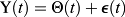
In this measurement equation, which in the state space modelling framework is referred to as the ‘observation equation’, the observed score Y(t) is decomposed into the true latent state level Θ(t) and a normally distributed error term ϵ(t).

To be able to obtain baseline, intraindividual variability, and attractor strength estimates for each individual, the BHOUM model has a hierarchical (or multilevel) character. This hierarchical structure allows the parameters of the BHOUM model to vary across participants. Apart from being hierarchical in nature, the model can also accommodate covariates. Those covariates can be time invariant, in which case the person–specific parameters (i.e. baseline, intraindividual variability, and attractor strength) are regressed on the time–invariant covariates. Another option is to include time–varying covariates, which can be done for the baseline only. Including such time–varying covariates in the prediction of the baseline allows the modelling of changes in the baseline level as a function of these covariates. Although the inclusion of covariates in the model is not required for testing the PersDyn model, they might be instrumental in examining why individuals differ in their level of trait baseline, intraindividual variability, and attractor strength.

To avoid computationally prohibitive integration of the numerous random effects' distributions, which are implied by the hierarchical nature of the model, the BHOUM model takes advantage of Bayesian statistical methods. In the Bayesian statistical framework, a posterior distribution is derived for each model parameter by combining a prior distribution with a likelihood function. Because in the Bayesian framework, parameters have (posterior) probability distributions, the Bayesian approach describes uncertainty about the parameters.² This can be done through the use of posterior credibility intervals (PCIs), which refer to the likelihood that the interval covers the true parameter value based on the observed data (Yuan & MacKinnon, 2009). In Bayesian modelling in general and in the BHOUM toolbox in particular, the combination of the prior distribution and the likelihood function is done using Markov chain Monte Carlo algorithms. Such Markov chain Monte Carlo algorithms iteratively update approximate distributions, which are improved in each step. Because of the iterative nature of the algorithm, one needs to specify how many iterations the sampling algorithm should execute. By default, the BHOUM toolbox performs 10 000 iterations, which should generally suffice for the models at hand (Oravecz, Tuerlinckx, & Vandekerckhove, 2012). Moreover, one should also specify how many of those iterations should be discarded when constructing the posterior distribution (i.e. the burn–in). In the BHOUM toolbox, this number is set to 4000 by default, which means that the first 4,000 iterations will not be taken into consideration. Finally, in the BHOUM toolbox, the Metropolis–within–Gibbs sampler is used, initiating several Markov chains from different starting values to avoid local optima. In the BHOUM toolbox, the number of Markov chains is set at six, which is typically considered enough (Oravecz et al., 2012).

Note that, given a particular sample size, estimation of some BHOUM parameters will be better (i.e. lower uncertainty in the parameter estimates) than estimation of other parameters. Although this topic has—to the best of our knowledge—not been studied yet, it is logical that the baseline estimate will be estimated with less uncertainty than the estimates of the higher order moments, such as variability and attractor strength.

To test the BHOUM model, Oravecz et al. (2012) developed a user–friendly graphical interface. The toolbox is available in two versions: as a standalone version and as a series of syntax files that can be run using MATLAB (both can be downloaded from https://sites.psu.edu/zitaoravecz/bayesian–ornstein–uhlenbeck–model/).

While the BHOUM model offers a straightforward way to test the PersDyn model, it was specifically developed for modelling two–dimensional phenomena (such as core affect; see Oravecz et al., 2011). Hence, it can only accommodate two–dimensional or—when running a two–dimensional model with the same variable loaded twice and imposing an independence constraint on the model (see Oravecz et al., 2012)—a unidimensional model. Thus, in case one wants to test a unidimensional model or a model that combines two personality dimensions—such as one of the combinations of the Abridged Big Five–Dimensional Circumplex model (Hofstee, De Raad, & Goldberg, 1992)—the BHOUM model might suffice. In case one wants to test higher dimensional models, the hierarchical continuous time dynamic model by Driver and Voelkle (2018) can be used. This model is similar to the BHOUM model, although there are some important differences. First, in the BHOUM model, the Β matrix (being the matrix containing the dynamic effects) is required to be symmetric and positive definite. This means that, in case of a two–dimensional model, the effects of the first process on the second one and vice versa are constrained to be equal. A consequence of this equality constraint is that the BHOUM model cannot accommodate damped linear oscillator or autoregressive and cross–lagged models because they require non–symmetric cross effects. Second, and more importantly, whereas the BHOUM model can accommodate for at most two dimensions, the hierarchical continuous time dynamic model by Driver and Voelkle has no theoretical upper limit in terms of the number of dimensions. Of course, one should be aware that with many dimensions, a large number of cross effects need to be estimated, which can only be done when the sample size is large enough. The hierarchical continuous time dynamic model by Driver and Voelkle, which can be tested using the ctsem R package (Driver, Oud, & Voelkle, 2017), thus offers a promising alternative to the BHOUM model.

Applying the Personality Dynamics Model to Experience Sampling Data on the Big Five

To illustrate the PersDyn model and the insights it can generate, we applied the model to experience sampling data from a study in which participants were asked to repeatedly fill out a Dutch version of Ten–Item Personality Inventory (Gosling, Rentfrow, & Swann, 2003; Hofmans, Kuppens, & Allik, 2008). Because the Big Five provide rather rough, high–level sketches of personality processes, this empirical example should not be conceived of as a study of the dynamic model of personality but rather as a tutorial–type illustration.³

This empirical example has purely exploratory example—there were no preregistered hypotheses.

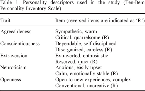
In terms of data collection, 1 week before the experience sampling started, participants received an online questionnaire with a Neuroticism–Extraversion–Openness Five–Factor Inventory personality assessment (Costa & McCrae, 1992). In the actual experience sampling study, questionnaires were sent five times a day between 10 am and 10 pm for seven consecutive days. At each beep, participants were instructed to rate the extent to which a number of personality descriptors applied to them (see Table 1 for the list of items). The items had to be rated on a 0–100 slider ranging from ‘strongly disagree’ to ‘strongly agree’. In the study, the order of the Ten–Item Personality Inventory questions was randomized. Sixty participants took part in the experience sampling study, yielding 1844 unique observations, which represents an average of 30.73 observations per participant. All measures, materials, and data used in this study are available via Open Science Framework link https://osf.io/t5v34/.

Table 1

Personality descriptors used in the study (Ten–Item Personality Inventory Scale)

Trait	Item (reversed items are indicated as ‘R’)
Agreeableness	Sympathetic, warm
	Critical, quarrelsome (R)
Conscientiousness	Dependable, self–disciplined
	Disorganized, careless (R)
Extraversion	Extraverted, enthusiastic
	Reserved, quiet (R)
Neuroticism	Anxious, easily upset
	Calm, emotionally stable (R)
Openness	Open to new experiences, complex
	Conventional, uncreative (R)

Analysis

Person–specific parameters of each of the five personality dimensions (i.e. baseline, variability, and attractor strength) were obtained by modelling the experience sampling data using five one–dimensional BHOUM models (Kuppens et al., 2010; Oravecz et al., 2016). For all analyses, we first divided the 0–100 score by 10, yielding raw scores between 0 and 10. Furthermore, item scores for items marked with an ‘R’ in Table 1 were reverse scored, after which we calculated scale scores for each Big Five dimension by taking the average score of the two items measuring that dimension.

In all models, we used the default BHOUM settings. That is, for each model, six chains were started (each starting from different starting values), with each chain consisting of 10 000 iterations. Burn–in, or the number of initial iterations that was discarded from the posterior distribution, was set to 4000.

Results

Trait Baseline

Table 2 provides a summary of the average baseline levels as well as the amount of interindividual variability in those baseline levels for each of the Big Five traits. For both parameters (average baseline and interindividual variability in baseline), we show both the posterior mean and the lower and upper limits for the symmetric 95% PCIs.

Table 2

Bayesian Hierarchical Ornstein–Uhlenbeck model parameters for baseline and interindividual variation in baseline. For both parameters, the posterior mean and the lower and upper limits for the symmetric 95% posterior credibility intervals are shown

	Baseline			Interindividual variation in baseline
	Posterior mean	95% PCI		Posterior mean	95% PCI
		LL	UL		LL	UL
A	7.67	7.48	7.86	.48	.30	.73
C	7.08	6.86	7.30	.69	.45	1.04
E	5.59	5.34	5.84	.72	.42	1.13
N	3.23	3.04	3.46	.64	.40	.99
O	5.52	5.33	5.71	.45	.27	.69

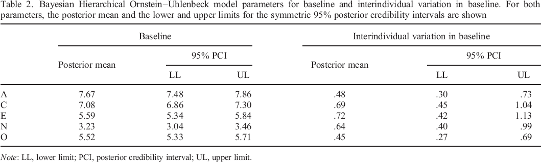
Note: LL, lower limit; PCI, posterior credibility interval; UL, upper limit.

As can be expected, the different Big Five dimensions differed in their average baseline level (see the baseline posterior means in Table 2). In terms of differences, Agreeableness and Conscientiousness had the highest average baseline values (being 7.67 for Agreeableness and 7.08 for Conscientiousness), while Neuroticism scored lowest. This means that the central point towards which one's behaviours, thoughts, and emotions converge over time are different for the different Big Five dimensions, a finding that fits well with previous research that showed the existence of significant differences across traits in the aggregated levels of momentary states (e.g. Fleeson, 2001; Jones, Brown, Serfass, & Sherman, 2017).

Apart from demonstrating the existence of between–trait differences in average baseline levels, our results also revealed that there were significant interindividual differences in baseline levels for each of the Big Five dimensions (see the Posterior means for interindividual variation in baseline). In other words, for each Big Five dimension, the central point towards which one's behaviours, thoughts, and emotions converge over time differs between individuals. The observation that there are large between–person differences on each of the Big Five dimensions is the cornerstone of the Big Five model and in the framework of the PersDyn model implies that trait baseline captures meaningful between–person variation in one's personality system.

Next, we computed correlations between the baseline values of the different Big Five traits (see Table 3). As can be seen in Table 3, the associations are higher than those found by previous studies (e.g. Meriac, Hoffman, Woehr, & Fleisher, 2008; Mount, Barrick, Scullen, & Rounds, 2005; De Raad et al., 2010). This suggests that trait baselines as derived from a series of state levels might be more closely related than trait levels as measured by typical personality inventories.

Table 3

Pearson's correlations for baseline levels of Big Five

	A	C	E	N
C	.68**
E	.51**	.46**
N	−.35**	−.31*	−.15
O	.45**	.49**	.55**	−.12

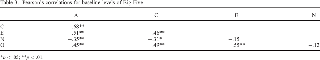
p < .05;

p < .01.

Trait Variability

Similar to the results for trait baseline, Table 4 provides a summary of the average level of intraindividual variation, while also showing interindividual differences in intraindividual variation for each of the Big Five traits. As is clear from Table 4, the extent to which people show within–person variability in their personality states is different for the different dimensions of the Big Five model. More specifically, Extraversion had the highest level of within–person variability, while the other traits had relatively comparable levels of within–person variability. In other words, relative to the other Big Five dimensions, people on average varied more on the Extraversion dimension across situations and time.

Table 4

Bayesian Hierarchical Ornstein–Uhlenbeck model parameters for intraindividual variability and interindividual variation in intraindividual variability. For both parameters, the posterior mean and the lower and upper limits for the symmetric 95% posterior credibility intervals are shown

Trait	Intraindividual variation			Interindividual variation in intraindividual variability
	Posterior mean	95% PCI		Posterior mean	95% PCI
		LL	UL		LL	UL
A	1.55	1.27	1.93	1.35	.49	3.21
C	1.80	1.42	2.37	2.97	1.05	8.02
E	3.66	2.79	4.56	4.61	1.70	11.33
N	2.07	1.55	2.75	3.97	1.20	11.66
O	2.29	1.72	3.03	5.46	1.76	16.09

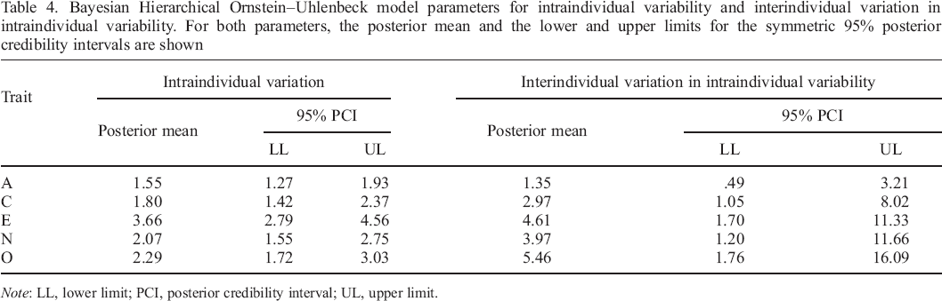
Note: LL, lower limit; PCI, posterior credibility interval; UL, upper limit.

By dividing the amount of interindividual variation in the baseline by the amount of intraindividual variation, one learns what percentage of the total (meaningful) variance is between individuals as opposed to within them. Note that this aligns with the calculation of intraclass correlation coefficient values in the multilevel regression framework, with the important difference that the BHOUM model separates intraindividual variation from measurement error, thereby providing a purer intraclass correlation coefficient measure. When applying this to the present data, we learn that 23.65% of the variance in Agreeableness, 27.71% in Conscientiousness, 16.44% in Extraversion, 23.62% in Neuroticism, and 16.42% in Openness is because of between–individual differences in the baseline, while the remainder is because of intraindividual differences in those personality dimensions.

Regarding individual differences in intraindividual variation—or the extent to which people differ in how much their trait–relevant behaviours, feelings, and cognitions differ across situations and time—significant between–person variation was found for each trait. This finding is particularly interesting because it aligns with the observation of Fleeson (2001) that the dispersion of a distribution of states is a meaningful individual difference variable. Moreover, this appears to hold true for each of the Big Five dimensions, with only minor (and non–significant) differences in the amount of interindividual variation in trait variability across traits (see the overlapping 95% PCIs for interindividual variation in intraindividual variability in Table 4).

In terms of correlations, all trait–specific intraindividual variabilities appeared to be significantly correlated (see Table 5). This might suggest that, although the amount of within–person variability differs across the different personality dimensions, there might be similar mechanisms that underlie these trait–specific intraindividual variabilities.

Table 5

Pearson's correlations relating intraindividual variability of the Big Five dimensions

	A	C	E	N
C	.50**
E	.39**	.54**
N	.60**	.42**	.29*
O	.26*	.39**	.61**	.37**

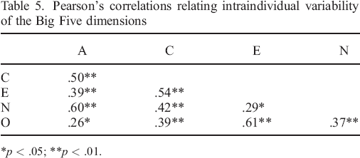
p < .05;

p < .01.

Trait Attractor Strength

As can be seen in Table 6, the force that pulls the individual back to their baseline appears to be dimension specific and is different for different individuals. Particularly, Agreeableness and Conscientiousness were characterized by both higher average levels of attractor strength and more between–person differences therein than the other Big Five dimensions. For Extraversion, Neuroticism, and Openness, the 95% PCI for interindividual variation in attractor strength included 0, implying that there were little between–person differences in attractor strength for those personality dimensions. Note that the BHOUM attractor strength estimates are not easily interpretable in an absolute sense. Whereas their magnitude and range might seem small, Oravecz, Tuerlinckx, and Vandekerckhove (2009) demonstrated that small differences in attractor strength have a large impact on the autocorrelation function (see figure 2 in Oravecz et al., 2009). To make matters even more complex, attractor strength estimates are affected by the time scale of the study. When studying minute–to–minute fluctuations, subsequent observations will be strongly correlated, while this will be less the case when studying day–to–day fluctuations, and this will be reflected in weaker attractor strength estimates in the former case. Because of those complexities, attractor strength is best interpreted in a relative rather than an absolute sense.

Table 6

Bayesian Hierarchical Ornstein–Uhlenbeck model parameters for attractor strength and interindividual variation in attractor strength. For both parameters, the posterior mean and the lower and upper limits for the symmetric 95% posterior credibility intervals are shown

Trait	Attractor strength			Interindividual variation in attractor strength
	Posterior mean	95% PCI		Posterior mean	95% PCI
		LL	UL		LL	UL
A	.040	.012	.156	.365	.001	1.036
C	.043	.013	.147	.081	.001	.172
E	.011	.005	.021	.000	.000	.003
N	.008	.003	.019	.000	.000	.004
O	.010	.006	.019	.000	.000	.001

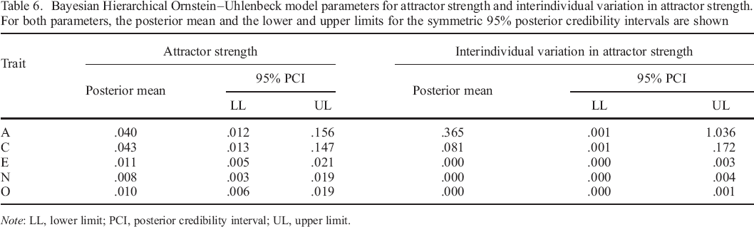
Note: LL, lower limit; PCI, posterior credibility interval; UL, upper limit.

Turning to the correlations between the attractor strength estimates for the different Big Five dimensions, we found that only attractor strengths of Agreeableness and Extraversion were significantly correlated (see Table 7). This again suggests that the third element of the PersDyn model, attractor strength, is trait specific.

Table 7

Pearson's correlations for attractor strength levels of Big Five

	A	C	E	N
C	.15
E	.28*	.14
N	−.11	−.05	.17
O	.13	−.10	.09	.05

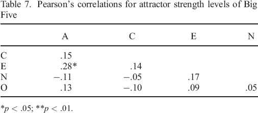
p < .05;

p < .01.

Finally, Table 8 shows the correlations between all elements of the BHOUM model for each of the Big Five traits.

Table 8

Pearson's correlations between baseline, variability, and attractor strength (att) parameters for each of the Big Five traits

		A		C			E			N			O
		Var	Att	Bas	Var	Att	Bas	Var	Att	Bas	Var	Att	Bas	Var	Att
A	Bas	−.31*	−.04	.68**	−.03	.01	.51**	.16	.10	−.35**	.04	.27*	.45**	.35**	−.02
	Var		.14	−.21	.50**	−.03	−.19	.39**	.26*	.11	.60**	−.01	−.12	.26*	.01
	Att			−.11	.04	.15	−.14	.20	.28*	.08	−.10	−.11	.04	.07	.13
C	Bas				−.46**	−.05	.46**	−.09	.03	−.31*	−.03	.22	.49**	.14	.01
	Var					.03	−.10	.54**	.11	−.01	.42**	−.15	−.11	.39**	−.03
	Att						.02	.02	.14	−.04	.01	.05	.10	.04	−.10
E	Bas							−.22	.08	−.15	−.05	.16	.55**	.11	.18
	Var								.14	−.27*	.29*	.01	−.18	.61**	.13
	Att									.24	.28*	.17	.20	.27*	.10
N	Bas										.26*	.03	−.13	−.09	.09
	Var											.03	.03	.37**	−.01
	Att												.11	.11	.05
O	Bas													.12	.04
	Var														.24

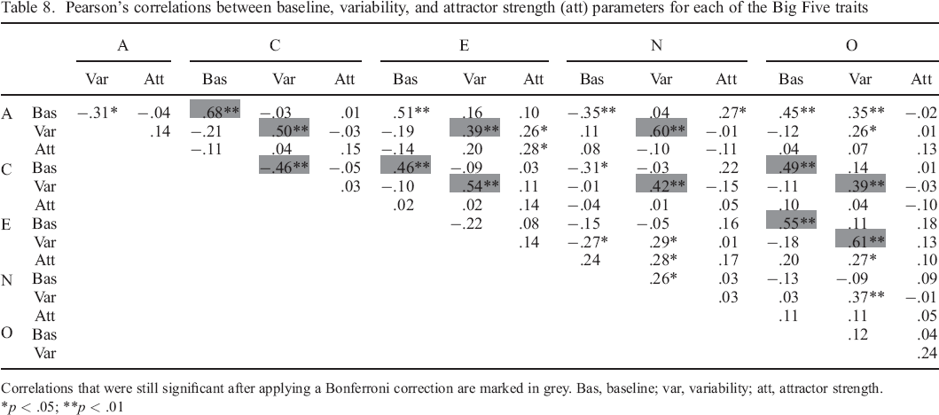
Correlations that were still significant after applying a Bonferroni correction are marked in grey. Bas, baseline; var, variability; att, attractor strength.

p < .05;

p < .01

New Insights and Implications

The proposed model offers several important implications for personality research. First and foremost, the PersDyn model provides a simple and straightforward way to apply dynamic systems principles to personality research by conceptualizing personality as a system in which the dynamics of the system—or the dynamic fluctuations in one's personality states—are governed by one's trait baseline, intraindividual variability, and trait attractor strength. By drawing on these three elements, the PersDyn model combines personality stability (i.e. attraction to one's trait baseline) and personality change (i.e. variability around this attractor). Central to this dynamic system conceptualization of personality is the concept of emergence—or the notion that general predispositions emerge from a series of momentary states.

The results obtained using the PersDyn model showed that each of the Big Five personality dimensions was characterized by high levels of both between–person variability in the baseline as well as within–person variability around this baseline. Moreover, and in line with previous studies that demonstrated that the amount of within–person variability in personality states is substantial (Fleeson, 2001), we found that all traits displayed higher levels of within–person than between–person variability. Note that in the PersDyn model, within–person variability is separated from measurement error (or unreliability; see Equation (2)), implying that this observation cannot be explained by the fact that the amount of within–person variation is confounded by measurement error. In the personality literature, there has been an ongoing discussion on whether within–person personality variability is trait specific or rather a general personality factor. While our results are of course indicative at best, the moderate correlations between the intraindividual variability scores for the different personality dimensions suggest that both mechanisms might co–exist. In particular, part of the variability might be due to a general variability factor, while some mechanisms underlying the amount of behavioural changes might also differ across traits. Further research might elaborate on this finding by testing whether the low correlations among the intraindividual variabilities are due to different underlying mechanisms or rather to differences in external factors that affect those traits’ variabilities.

Through the inclusion of a temporal dimension, the PersDyn model accounts for self–regulation of momentary fluctuations in one's personality system. In the PersDyn model, self–regulation takes the form of a return to the baseline (i.e. it is assumed that people over time will return to their baseline level). The inclusion of self–regulation in the model is an important contribution to the personality literature because such self–regulatory mechanisms, and particularly individual differences therein, have so far received less attention compared with baseline personality and personality variability. In terms of empirical findings, the results on attractor strength seem to suggest that these self–regulatory mechanisms might be trait specific. That is, the non–significant correlations between the attractors strengths of different traits suggest that mechanisms that underlie regulatory processes might be different for each trait. It must be pointed out though that the nature of attractor strength for each trait warrants further research, especially considering that there were very little between–person differences in attractor strength for Extraversion, Openness, and Neuroticism. Moreover, it is important to note that the strength of an attractor can be modelled in other ways as well, with one example being models that predict change in personality states as an outcome (see Danvers, Wundrack, & Mehl, 2019).

Conclusion

In this paper, we offered a dynamic systems approach to personality as a new way of conceptualizing and assessing individual differences. Based on intensive longitudinal data on the Big Five personality traits, we showed that there are meaningful individual differences in the model's parameters, namely baseline, variability and attractor strength and that the patterns of change in personality states differed on both the between– and within– person level. Secondly, we provided an overview of tools necessary to examine the temporal dynamics of such individual differences, including a discussion of both the required study designs and statistical analysis. Altogether, we conclude that the dynamic systems perspective has a potential to integrate research on stable and dynamic elements of personality and advance the knowledge on personality processes, by focusing on both momentary expressions and stable patterns within individuals simultaneously.

Supporting Information

Supporting Information, PER2233 - New Directions in the Conceptualization and Assessment of Personality—A Dynamic Systems Approach

Supporting info item

Supporting Information, PER2233 for New Directions in the Conceptualization and Assessment of Personality—A Dynamic Systems Approach by JOANNA SOSNOWSKA, PETER KUPPENS, FILIP DE FRUYT and JOERI HOFMANS, in European Journal of Personality

Supporting info item

Footnotes

Supporting Information

Additional supporting information may be found online in the Supporting Information section at the end of the article.

References

Barrick

M. R.

, Mount

M. K.

, & Judge

T. A.

(2001). Personality and performance at the beginning of the new millennium: What do we know and where do we go next? International Journal of Selection and Assessment, 9, 9–3. https://doi.org/10.1111/1468–2389.00160.

Baumert

, Schmitt

, Perugini

, Johnson

, Blum

, Borkenau

, … Wrzus

(2017). Integrating personality structure, personality process, and personality development: Integrating personality. European Journal of Personality, 31, 503–528. https://doi.org/10.1002/per.2115.

Beal

D. J.

, & Weiss

H. M.

(2003). Methods of ecological momentary assessment in organizational research. Organizational Research Methods, 6, 440–464. https://doi.org/10.1177/1094428103257361.

Costa

P. T.

Jr. , & McCrae

R. R.

(1992). The revised NEO Personality Inventory (NEO PI–R) and NEO Five–Factor Inventory (NEO–FFI) professional manual. Odessa, FL: Psychological Assessment Resources.

Danvers

, Wundrack

, & Mehl

M. R.

(2019). Equilibria in Personality States: A Conceptual Primer for Dynamical Analyses.

Dalal

R. S.

, Meyer

R. D.

, & Bradshaw

R. P.

(2015). Personality strength and situational influences on behavior: A conceptual review and research agenda. Journal of Management, 27, 261–287. https://doi.org/10.1177/0149206314557524.

De Raad

, Barelds

D. P.

, Levert

, Ostendorf

, Mlačić

, Blas

L. D.

, Hrebícková

, … Church

A. T.

(2010). Only three factors of personality description are fully replicable across languages: A comparison of 14 trait taxonomies. Journal of Personality and Social Psychology, 98, 160–173. https://doi.org/10.1037/a0017184.

DeYoung

C. G.

(2015). Cybernetic Big Five Theory. Journal of Research in Personality, 56, 33–58. https://doi.org/10.1016/j.jrp.2014.07.004.

Driver

C. C.

, Oud

J. H. L.

, & Voelkle

M. C.

(2017). Continuous time structural equation modeling with R package ctsem. Journal of Statistical Software, 77. https://doi.org/10.18637/jss.v077.i05.

10.

Driver

C. C.

, & Voelkle

M. C.

(2018). Hierarchical Bayesian continuous time dynamic modeling. Psychological Methods. Advance online publication. https://doi.org/10.1037/met0000168.

11.

Ebner–Priemer

U. W.

, & Trull

T. J.

(2009). Ambulatory assessment: An innovative and promising approach for clinical psychology. European Psychologist, 14, 109–119. 1.1027/1016–904.14.2.109.

12.

Fisher

C. D.

, & To

M. L.

(2012). Using experience sampling methodology in organizational behavior: Experience sampling methodology. Journal of Organizational Behavior, 33, 865–877. https://doi.org/10.1002/job.1803.

13.

Fleeson

(2001). Toward a structure–and process–integrated view of personality: Traits as density distributions of states. Journal of Personality and Social Psychology, 80, 1011. https://doi.org/10.1037/0022–3514.8.6.1011.

14.

Fleeson

(2017). The production mechanisms of traits: Reflections on two amazing decades. Journal of Research in Personality, 69, 4–12. https://doi.org/10.1016/j.jrp.2017.07.003.

15.

Fleeson

, & Jayawickreme

(2015). Whole trait theory. Journal of Research in Personality, 56, 82–92. https://doi.org/10.1016/j.jrp.2014.10.009.

16.

Furr

(2009). Profile analysis in person–situation integration. Journal of Research in Personality, 43, 196–207. https://doi.org/10.1016/j.jrp.2008.08.002.

17.

Gosling

S. D.

, Rentfrow

P. J.

, & Swann

W. B.

Jr. (2003). A very brief measure of the Big–Five personality domains. Journal of Research in Personality, 37, 504–528. https://doi.org/10.1016/S0092–6566(03)00046–1.

18.

Hofmans

, De Clercq

, Kuppens

, Verbeke

, & Widiger

T. A.

(2019). Testing the structure and process of personality using ambulatory assessment data: An overview of within–person and person–specific techniques. Psychological Assessment, 31, 432–443. https://doi.org/10.1037/pas0000562.

19.

Hofmans

, Kuppens

, & Allik

(2008). Is short in length short in content? An examination of the domain representation of the ten item personality inventory scales in Dutch language. Personality and Individual Differences, 45, 750–755. https://doi.org/10.1016/j.paid.2008.08.004.

20.

Hofstee

W. K.

, De Raad

, & Goldberg

L. R.

(1992). Integration of the Big Five and Circumplex approaches to trait structure. Journal of Personality and Social Psychology, 63, 146–163. https://doi.org/10.1037/0022–3514.63.1.146.

21.

Jones

A. B.

, Brown

N. A.

, Serfass

D. G.

, & Sherman

R. A.

(2017). Personality and density distributions of behavior, emotions, and situations. Journal of Research in Personality, 69, 225–236. https://doi.org/10.1016/j.jrp.2016.10.006.

22.

Judge

T. A.

, Simon

L. S.

, Hurst

, & Kelley

(2014). What I experienced yesterday is who I am today: Relationship of work motivations and behaviors to within–individual variation in the five–factor model of personality. Journal of Applied Psychology, 99, 199–221. https://doi.org/10.1037/a0034485.

23.

Kuppens

, Oravecz

, & Tuerlinckx

(2010). Feelings change: Accounting for individual differences in the temporal dynamics of affect. Journal of Personality and Social Psychology, 99, 1042–1106. https://doi.org/10.1037/a0020962.

24.

Lee

, & Ashton

M. C.

(2004). Psychometric properties of the HEXACO personality inventory. Multivariate Behavioral Research, 39, 329–358. https://doi.org/10.1207/s15327906mbr3902_8.

25.

McCrae

R. R.

, & Costa

P. T.

Jr. (1999). A five–factor theory of personality. In Pervin

L. A.

, & John

O. P.

(Eds.), Handbook of personality: Theory and research (pp. 139–153). New York, NY, US: Guilford Press.

26.

Meriac

J. P.

, Hoffman

B. J.

, Woehr

D. J.

, & Fleisher

M. S.

(2008). Further evidence for the validity of assessment center dimensions: A meta–analysis of the incremental criterion–related validity of dimension ratings. Journal of Applied Psychology, 93, 1042–1052. https://doi.org/10.1037/0021–901.93.5.1042.

27.

Mount

M. K.

, Barrick

M. R.

, Scullen

S. M.

, & Rounds

(2005). Higher–order dimensions of the big five personality traits and the big six vocational interest types. Personnel Psychology, 58, 447–478. https://doi.org/10.1111/j.1744–657.2005.00468.X.

28.

Ones

D. S.

, & Viswesvaran

(1996). Bandwidth–fidelity dilemma in personality measurement for personnel selection. Journal of Organizational Behavior, 17, 609–626. https://doi.org/10.1002/(SICI)1099–1379(199611)17:6<609::AID–JOB1828>3..CO;2–K.

29.

Oravecz

, Tuerlinckx

, & Vandekerckhove

(2011). A hierarchical latent stochastic differential equation model for affective dynamics. Psychological Methods, 16, 468–449. https://doi.org/10.1037/a0024375.

30.

Oravecz

, Tuerlinckx

, & Vandekerckhove

(2016). Bayesian data analysis with the bivariate hierarchical Ornstein–Uhlenbeck process model. Multivariate Behavioral Research, 51, 106–119. https://doi.org/10.1080/00273171.2015.1110512.

31.

Oravecz

, Tuerlinckx

, & Vandekerckhove

(2012). User's guide to the BHOUM software.

32.

Shoda

, LeeTiernan

, & Mischel

(2002). Personality as a dynamical system: Emergence of stability and distinctiveness from intra and interpersonal interactions. Personality and Social Psychology Review, 6, 316–325. https://doi.org/10.1207/S15327957PSPR0604_06.

33.

Sosnowska

, Kuppens

, De Fruyt

, & Hofmans

(2019). A dynamic systems approach to personality: The Personality Dynamics (PersDyn) model. Personality and Individual Differences, 144, 11–18. https://doi.org/10.1016/j.paid.2019.02.013.

34.

Trull

T. J.

, & Ebner–Priemer

(2013). Ambulatory assessment. Annual Review of Clinical Psychology, 9, 151–176. https://doi.org/10.1146/annurev–clinpsy–050212–185510.

35.

Trull

T. J.

, & Ebner–Priemer

(2014). The role of ambulatory assessment in psychological science. Current Directions in Psychological Science, 23, 466–447. https://doi.org/10.1177/0963721414550706.

36.

Vallacher

R. R.

, Nowak

, Froehlich

, & Rockloff

(2002). The dynamics of self–evaluation. Personality and Social Psychology Review, 6, 370–379. https://doi.org/10.1207/S15327957PSPR0604_11.

37.

Voelkle

M. C.

, & Oud

J. H.

(2013). Continuous time modelling with individually varying time intervals for oscillating and non–oscillating processes. British Journal of Mathematical and Statistical Psychology, 66, 103–126. https://doi.org/10.1111/j.2044–8317.2012.02043.X.

38.

Yuan

, & MacKinnon

D. P.

(2009). Bayesian mediation analysis. Psychological Methods, 14, 301–322. https://doi.org/10.1037/a0016972.