
Abstract
Cooperative control of multiple mobile robots is an attractive and challenging problem which has drawn considerable attention in the recent past. This paper introduces a scalable decentralized control algorithm to navigate a group of mobile robots (swarm) into a predefined shape in 2D space. The proposed architecture uses artificial forces to control mobile agents into the shape and spread them inside the shape while avoiding inter-member collisions. The theoretical analysis of the swarm behavior describes the motion of the complete swarm and individual members in relevant situations. We use computer simulated case studies to verify the theoretical assertions and to demonstrate the robustness of the swarm under external disturbances such as death of agents, change of shape etc. Also the performance of the proposed distributed swarm control architecture was investigated in the presence of realistic implementation issues such as localization errors, communication range limitations, boundedness of forces etc.
Keywords
Introduction
With recent advances in communication, networking and computing, multi-agent systems have generated a renewed interest among researchers across the world (Chaimowicz, Michael et al. 2005; Chao-xia, Bing-rong et al. 2007; De Gennaro, Iannelli et al. 2005; Desai, Ostrowski et al. 1998; Gazi and Passino 2002; Kwok, Ha et al. 2007; Ramani, Viswanath et al. 2008; Suzuki and Yamashita 1999; Xin and Yangmin 2008). Although swarm or multi-agent dynamic system concept, in general, is used in several disciplines, this work considers a multi-agent system as a collection of loosely coupled dynamic units moving in 2 or 3 dimensional space. In applications, the dynamic units can be robots, vehicles, UAVs, etc, where the motion dynamics is governed by a common control algorithm. These systems (robotic colonies/swarming robots) are fundamentally designed to perform a task in a cooperative fashion, requiring integrated decision making facilitated by effective peer-to-peer communication (Sycara 1998). Multi-agent systems (MAS) have distinct advantages and unique applications over single agent based systems due to reduced cost and unit size. In particular, defense applications employing disposable mobile sensory nodes for spying purposes have added advantages due to multiplicity and spacial diversity of agents.
Natural swarms or social foraging animal groups that perform extensive amounts of group work and survive as a powerful society (i.e. ant colonies, bees etc) provide convincing conceptual framework in the area of multi-agent systems. Autonomous behavior (without a central control) of natural swarms such as ant colonies (Gordon 2003) have motivated researchers to mimic natural systems. Many researchers studied group behavior of animals such as organization of work in ant colonies (Gordon 2003), social foraging models in fish (Hamilton and Dill 2003), navigation and signaling methods used by ants (Robinson, Jackson et al. 2005) and shoaling behavior of fish (Brown and Warburton 1999) with respect to performing an escape mechanism. Mathematical models for the group behavior developed by Inada in (Inada 2001) and algorithms governing schooling behavior of fish presented by Grunbaum et al. (Grünbaum 2004) etc, have inspired the robotics researchers into more refined approaches in swarming techniques (Krieger, Billeter et al. 2000; Kwok, Ha et al. 2007; Ramani, Viswanath et al. 2008).
Aggregation and formation are among the most important behaviors exhibited by biological swarms which enable them to protect against natural threats, strengthen them with sensing capabilities to locate food, resources, escape routes, etc (Brown and Warburton 1999). As the artificial swarms can gain similar benefits from such behavior, robotic and multi-agent system researchers have introduced various formation models. A formation strategy based on inter-agent attraction/repulsion function was proposed by Gazi et al in (Gazi and Passino 2003) and (Gazi and Passino 2002) together with a stability analysis of the flocking algorithm. Also Gazi proposed a multi-agent formation using a similar attraction/repulsion profile combined with artificial potentials in (Gazi 2005). Apart from the inter-agent forces, a behavior based formation model was introduced by Balch et al in (Balch and Arkin 1998). Soyal and Sahin (Soysal and Sahin 2005) also introduced a behavior based generic aggregation method using simple reactive behaviors of the agents. While a rather different approach was introduced by Naruse et al (Naruse, Yokoi et al. 2003) for aggregation of multi-agent systems; they used emotion-like two dimensional inner state and affection-like subjective evaluation of others to perform aggregation behavior. Olfati-Saber in (Olfati-Saber 2006) presented a comprehensive theoretical framework for a multi-agent aggregation. In his paper distributed algorithms for free-flocking (i.e. flocking where obstacles are not present) and constrained flocking (i.e. in presence of obstacles) are introduced and the behavior is analysed. Formation, where a specific shape is formed (Harry Chia-Hung and Liu 2005), is also a critical aspect in MAS research, because it facilitates easy maneuvering of the whole MAS when it comes to path planning and strategic positioning (especially in military applications). Many researchers developed and analyzed models for formation control and navigation of multi-agent systems. For example, in (Balch and Arkin 1998), the authors describe a behavior based formation and navigation method for autonomous land vehicles, whereas in (Kalantar and Zimmer 2004), the authors presented a contour shaped formation control method for autonomous underwater vehicles. Leader based pattern formation of a group of robots in (Desai, Ostrowski et al. 1998; Huang, Farritor et al. 2006; Tanner, Pappas et al. 2004; Yang and Gu 2007), Neural network based path planning and assembly (Xiaobu and Yang 2007), geometric pattern formation of multi-agent systems using a decentralized controller in (Bishop 2003; Lawton, Beard et al. 2003; Stilwell, Bishop et al. 2005; Suzuki and Yamashita 1999) and positioning strategies in pattern transitions of MAS described in (Spletzer and Fierro 2005) use a rather different approach to the artificial potential field based formation control model introduced in (Gazi 2005). In (Shuzhi Sam, Chency-Heng et al. 2004), the authors introduce generalized artificial potential functions for swarm shape formations. The stability analysis of swarms under formation algorithms were considered in (Gazi and Passino 2003; Gazi and Passino 2004; Tanner, Pappas et al. 2004; Yang, Passino et al. 2003; Yang, Passino et al. 2003), some providing bounds on swarm sizes, time of formation etc,. In (Antonelli and Chiaverini 2006) the authors present a centralized scheme for controlling a platoon of autonomous vehicles, which demonstrate abilities such as obstacle avoidance, target tracking etc.
In this paper we present a decentralized aggregation and shape formation scheme for a multi-agent society that will converge into a predefined shape in 2D space. Our approach is decentralized in the sense that mobile agents do not need constant communication with a base station, which does the path planning and send navigation commands (as in (Antonelli and Chiaverini 2006)). Instead we use communication between mobile agents, self localization capabilities, predetermined targets and parameters; which enable mobile agents to plan the path on their own. Under the proposed control architecture we populate a given shape (rather than the periphery as in (Chaimowicz, Michael et al. 2005; Hsieh and Kumar 2006; Suzuki and Yamashita 1999; Yang, Passino et al. 2003)) with the swarm without using predefined positions (unlike in (Desai, Ostrowski et al. 1998; Spletzer and Fierro 2005)). The shapes can be described by a mathematical function (contour). This paper is based on our previous work which appeared in (Ekanayake and Pathirana 2006), which introduces an aggregation algorithm for a swarm of robots. In (Ekanayake and Pathirana 2007; Ekanayake and Pathirana 2008), we present an application of the shape formation algorithm used for controlling an airborne weapon system. The formation algorithm uses inter-agent repulsion forces in order to avoid collisions between agents, global formation forces which converges the swarm into the predetermined shape and a friction-like damping force that brings the swarm to a halt once the swarm is distributed inside the shape.
An outline of the paper is as follows: In section 2 we introduce the swarm model and analyse the behavior with certain assumptions. Here the model assumes the agents as point objects with no physical dimensions but with identical physical properties (such as mass, mobility, etc,.). Also in order to reduce the system complexity and highlight the formation algorithm, we assume error free and instantaneous localization capabilities. Then in section 3 we discuss the implementation considerations of the proposed algorithm. Here we introduce a modified controller to avoid obstacles, facilitate agent size and actuator limitations. Also we discuss the additional constraints affecting the performance of the formation algorithm together with an implementation procedure. With the simulation case studies presented in section 4, we verify the claims proposed in section 2 and demonstrate the behavior with constraints and modified models discussed in section 3. Finally, with concluding remarks (section 5) we state directions to possible future work in this area.
Swarm Model and the Controller Analysis
The swarm model with basic artificial forces is introduced followed by a mathematical analysis of the swarm behavior. For the analysis, the following were assumed;
Agents/members have identical physical properties (such as mass, mobility etc.) Agents/members are point masses i.e. without any physical dimensions and demonstrate point mass dynamics Agents/members have instantaneous and error free localization capabilities The communication network of the members can transmit data to all the members within the group instantaneously, i.e. without delay (see (Ekanayake, Pathirana et al. 2008)) Agents/members operate on a flat surface without obstacles
Basically the above assumptions were made in order to reduce the system complexity in the controller analysis phase and to highlight the basic formation algorithm. But in subsequent sections of the paper we relax these assumptions and use a swarm model which closely resembles a platoon of real world robotic vehicles.
Throughout this paper, the terms member or agent represent a member in the swarm, while the terms swarm or multi-agent system represents the complete swarm. Also, we use
Remark
For easy representation of vector based force components with contour integrals and for ease of analysis we used the complex plane instead of the cartesian plane. But in implementing the algorithm in real robots, the cartesian vector based representations can be adopted.
Basic Aggregation and Shape formation Model
Consider a swarm or multi-agent system consisting of N number of identical members operating in two dimensional Euclidean space. In this context we consider the problem of controlling and positioning the above swarm into a shape bounded by a simple closed contour γ defined in the complex plane, while spreading members inside the contour uniformly.
The state of the member i is described by
where z
i
∈ C, represents the position of the i
th
member in 2D complex plane. Let z be a point on γ, i.e. z ∈ γ. Before stating the swarm model, we define α = [1 0] and β = [0 1]. Then the state of the whole swarm, x =[X1 X2 X3 … X
N
]
T
is determined by the continuous time dynamic model described by,

where


with

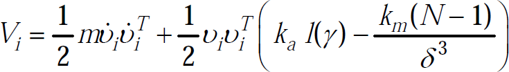
In (4), m is the mass of a member. According to our assumptions, notice that each member's position information
The control input u in (2) consists of,

where

The artificial formation forces are described as follows; F
i,a
, attraction force on the i
th
member from the shape,
F
i,r
, artificial repulsion force on the i
th
member from the shape,

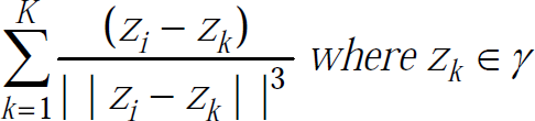
In above equations, n(γ,z
i
) represents the Cauchy Winding Number of γ about z
i
∈

Remark
Clearly,

ensures that the term F i,a in (7) vanishes only if the member is inside the contour and term F i,r vanishes only if member is outside the shape.
F
i,m
in (7) refers to the resultant force acting on the i
th
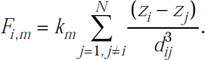
member from the remaining members of the swarm (inter member repulsion force), i.e:

F
i,f
in (7) is given by,
and k
a
,k
r
,k
m
,k
f
∈
For notational simplicity, we use F i,a , F i,r , F i,f and F i,m terms instead of functional F i,a (x i ,γ), F i,r (x i ,γ), F i,f (x i ) and F i,m (x i ) respectively.
F i,r and F i,a in (7) are the artificial force fields on each member, forcing them towards the desired shape and evenly distributing them inside the contour. F i,m term in the control function avoids the inter-member, collisions. The inter member interaction function looks similar to the repulsive term described in (Gazi 2005; Gazi and Passino 2003), etc. except that the problem of decreasing repulsion behavior for small inter member distances is avoided by our repulsion term; thus preventing collision among agents. F i,f is the artificial friction force exerted on each member, forcing the member to a complete stop when the artificial formation forces are balanced. This is to ensure that the agents reach a desirable static equilibrium state.
Total force acting on an individual member makes it travel toward the shape when it is outside the shape and will converge toward a stable position when it is inside the shape. As the formation force components (F i,r and F i,a ) do not act simultaneously, we can analyze the behavior and the stability of the controller in each instance separately. In section 2.2.1, we first analyse the behavior of the complete swarm when all the members are outside the shape, i.e. when every member is subjected to F i,a force. Next, we analyse the behavior of a member staying outside the shape, with claims on the direction of motion. With analysis of the behavior of a single member inside the shape contour, in section 2.2.2., we provide equilibrium position(s) inside a shape contour symmetrical over two or more axes. Then we discuss the results with logical explanations on the swarm behavior in specific situations (section 2.3.).
Before analysing the behavior of the swarm, we define the following;

where z cm , z c and l(γ) represent the center of mass of the swarm, the center of mass of the contour and length of the contour respectively.
Firstly, we examine the behavior of the swarm, when all the members are outside the contour. In our analysis, the swarm is considered as one object in which the motion is governed by the resultant artificial force (R),

With this, the equation of motion of the whole swarm can be described by,

where ɛ = (z
cm
- z
c
),
Notice that in (13); R
m
, which represents the resultant inter member force is zero as,
R
a
, the resultant artificial attraction force from the contour, is expressed as,

and using definitions for z
c
, z
cm
and l(γ), the above can be stated as:

R
f
, represents the resultant artificial damping (friction) force, and is in the form of,

Therefore, the net resultant force on the swarm (this force is applied on the center of mass of the swarm) is,

and hence the motion dynamics of the swarm can be described by (14).
With the above motion dynamics of the whole swarm, we obtain our first result; the center of mass of the swarm (z cm ) moves towards the shape. This is given in the form of the following theorem.
Theorem 1
Consider the swarm model described by (14), motion of the center of mass of the swarm (z cm ) is in the direction of decreasing ɛ (i.e. toward the center of mass of the contour z c ).
Proof
If we select a Lyapunov function candidate as
Since
Basically, this theorem says that the motion of the center of mass of the complete swarm is toward the center of mass of the contour and this holds, regardless of the motions of members with respect to z cm . Note that Theorem 1 does not hold, if any member of the swarm moves into the shape.
Remark
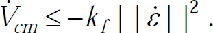
Using the properties of second order ODEs one can state that; smooth motion of the swarm (i.e. damped motion dynamics) towards the target contour (z
c
) can be obtained if the conditions m,k
a
,k
f
>0 and
Theorem 1 shows only the behavior of the swarm, but it does not say anything about the behavior of an individual agent. Next we investigate the behavior of the members in a specific swarm, where the members have a predefined minimum spacing: “X Swarm”. Further, we introduce a condition for a “X Swarm” to be cohesive under F i,a force in the theorem to follow.
Definition 1
A swarm S is defined as “X swarm”, if there exists positive constants Δ,δ that satisfy the following conditions simultaneously for all i,j ɛ S and i ≠ j.
d
ij
⩾ δ + Δ,

In the above,
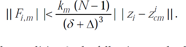
In the first condition of the “X Swarm” definition, we impose a constraint on the distance between robots in a group. That is the distance d i,j is larger than a selected value (δ + Δ). From the second condition we set the ratio between δ and Δ, in which the ratio can be made to move toward zero with the increasing size of the swarm. Using the definition of “X Swarm” we derive that the inter member repulsion force (F i,m ) on any member of the swarm is bounded, as presented, in following lemma.
Lemma 1
For a member of a “X Swarm”, the magnitude of the artificial inter-member repulsion force is less than

Proof
Using the condition 1 of the “X Swarm”, we have
Then using the condition 2, the following can be derived;
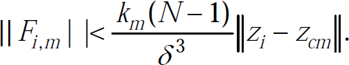
The above result is an upper bound for the magnitude of the inter member repulsion force F
i,m
in a “X swarm”, which we use in the proceeding sections. Before investigating more into the behavior of a single member, we define the error between z
i
and z
cm
as v
i
= (z
i
- z
cm
); resulting

in which we used,

as n(γ, αX i ) = 0.

which describes the motion of a single agent with respect to the center of mass of the swarm. In the following theorem we introduce a condition for a “X Swarm” to be cohesive under F i,a with a member having motion dynamics given by (21). Also with this condition we can describe the direction of motion of any member of a “X Swarm” outside the shape.
Theorem 2
Consider a member i of a “X Swarm” staying outside the desired shape at any given time, if
Proof
Choosing a Lyapunov function candidate for the member i as
and taking derivatives, we can show that

Since we consider a member of a “X Swarm”, from Lemma 1,

and hence,

which proves the assertion.
This theorem describes the motion of a robot which is a member of a “X Swarm” and staying outside the shape. To satisfy the above conditions, there is no restriction on the positions of the other members of the swarm or the position of z cm , i.e. they may either be inside or outside the target shape.
Remark
Consider a group of robots released far away from the desired shape, having an artificial force based controller described in (7) and satisfying “X Swarm” hypothesis. In general terms theorems 1 and 2 infer that the robots (members) move toward the shape.
So far we have analyzed the behavior of the swarm and individual members staying outside the contour. In this section we investigate the behavior of F i,r formation force acting on an agent, where the contour γ is symmetrical over one or more strait lines. Then we comment on the stable location of the swarm.
Remark
Since any 2D shape can be generated using several symmetrical shapes, we analysed the behavior only for symmetrical shapes. The analysis can easily be extended to non symmetric shapes, considering them as a collection of symmetric shapes.
In the following lemma, we use odd and even function properties to derive a property of a complex function which is symmetrical over real axis of the complex plane.
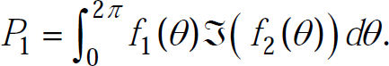
Lemma 2
For a closed contour γ(θ) and functionals f1(θ) ɛ

the following statement holds,

Proof
Let

as f1(θ)ɛ
Since f1(θ) and
Before stating our result about a member, we discuss the nature of the artificial formation force, F
i,r
in detail.
and

In our analysis we define,

Using polar coordinate representation for complex plane, we reformulate F
i,r
as

which is used to prove our next results.
Theorem 3
Consider a member i inside a given contour γ(θ) with the following properties:
γ(θ) = γ*(2π − θ),
Then,

Proof
F
i,r
in equation (32), have the following properties when


thus using Lemma 2,

Above result say that for any member i staying on the real-axis and inside the shape, which is symmetrical around the real-axis, the component of F i,r parallel to the imaginary axis is zero. In other words, the F i,r force on that member is along the real axis. Further we extend the above result to a shape with an axis of symmetry other than the real-axis and then prove that the equilibrium point lies on the intersection of the symmetric axes, as shown in the following Theorem.
Theorem 4
Consider a given contour γ(θ) = r(θ)eiθ with two symmetric axes. Then, for a member i staying on the intersection of the symmetrical axes, the artificial repulsion force from the contour (F i,r ) is zero.
Proof
Consider two symmetric axes (k,l) form α
k
,α
l
∈ [0,2π] angles to the real axis. Assume the member is on the intersection of the symmetric axes. Then, from Theorem 3, F
i,r
is in the form of:

where μ
k
,μ
l
∈
Above result states that, for a contour symmetrical over two intersecting straight lines, there exists a point, where F i,r = 0. In other words, the intersection point of symmetric axes is a possible equilibrium point for the member moving under F i,r artificial formation force. Our computer simulations confirm these assertions. (refer Fig. 1.)
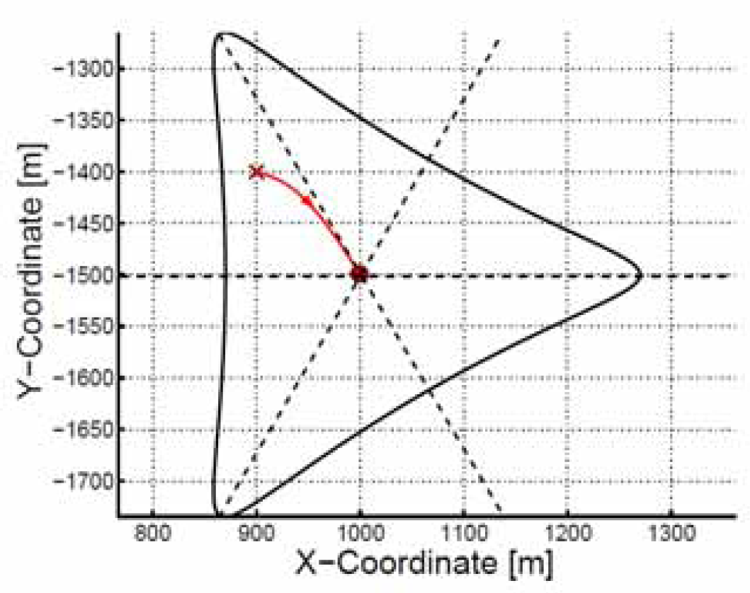
Motion of a single agent under F i,r force. (Dotted lines represent symmetical axes)
Remark
The analysis of the motion of a single member can be extended to determine the behavior of the complete swarm (when all agents are inside the shape). By considering the complete swarm as one object with the center of mass of the swarm being the center of the object, we can conclude that the swarm will have a stable equilibrium under F i,r force, with the center of mass of the swarm moved to the center of mass of the contour which is symmetrical over a minimum of two intersecting straight lines (see Fig. 2.).

Motion of the whole swarm inside the contour. The motion of the center of mass of the weapons is represented in black while red lines represent the motion path of individual members. The initial and final positions are represented by a cross and a dot respectively. Dotted lines represent symmetical axes)
In the previous sections the behavior of the swarm and individual members were analysed for the following cases (the summarized results are given below);
Center of mass of the swarm (z cm ): If all the members are outside the shape, the motion of the center of mass of the swarm (z cm ) is towards the center of mass of the contour (z c ).
A member outside the shape: With the “X Swarm” assumptions and conditions on theorem 2 remain true, the motion of an individual will be towards the center of mass of the swarm.
Inside a symmetrical shape:
A member will have a stable equilibrium point on the symmetrical axis. Further, if the shape has two or more intersecting axes, then the stable equilibrium point lies on the intersection of the axes.
When all the members are inside the shape, then the motion of the center of mass of the swarm (z cm ) will have a stable equilibrium point on the symmetrical axis. As in the previous case, this stable equilibrium point lies on the intersection of the symmetrical axes.
Next we focus our attention to the aspects which were not considered in the mathematical analysis provided in the previous sections. When a section of the swarm is inside the contour we can use theorem 2 to describe the motion of a member outside the contour, provided that the swarm behaves as “X Swarm”. A swarm which does not satisfy the condition;
A major drawback of the controller is the discontinuous nature of the artificial formation forces (i.e. F i,r and F i,m ), which may cause chattering effect at the boundary of, the shape. Since the term n(γ, αX i ) is not defined on the contour, the member will continue its motion using the previous motion dynamics until it passes the boundary. Since the boundary is a line without a thickness, this problem will not be a significant unless a member is on the boundary at the beginning. However, the inter member forces acting on such members does not allow them to be on the contour once the algorithm is initialized. Also, as shown in the Fig. 3., the formation forces (F i,a and F i,r ) which drives the members into the contour has a significant variation at the boundary. Specially the decreasing magnitude of the driving force when a member is staying closer but outside of the contour, may result in the member to staying outside the contour at the equilibrium state. This happens only when the contour is not large enough to accommodate all the members, thus F i,m becomes larger than F i,a such that some members are not allowed in. This problem can be eliminated by carefully selecting k a and k m parameters which suit the application and the swarm size.

Behavior of “Artificial Formation Forces” at the contour boundary. The red and black lines represents the variation of F i,a and F i,r forces respectively. For better visualization of the changes in two forces, the F i,r force is limited up to 5000N.
In this section we discuss the issues to be considered when implementing the proposed architecture in a real world scenario. The shape formation algorithm can effectively be used in the navigation of air launched weapon systems (as in (Ekanayake and Pathirana 2007; Ekanayake and Pathirana 2008)), control of full sized wheeled/tracked robots in military operations, cooperative positioning of “de-mining robots” etc. However in this discussion, we are not considering a specific application, instead we present modifications and discuss other implications for the general case. First we discuss the modifications for the controller in order to compensate for the implications with practical implementation of (7). Further the implications due to the assumptions (in (7)) are discussed together with possible remedial approaches using realistic error models implemented in the simulation case studies.
Controller Modification for Practical Implementation
Upon the introduction of the controller and in the behavioral analysis of the multi-agent system, we considered the members as point masses (i.e. without any physical dimensions) and assumed that they can exert virtually any artificial force (i.e. unbound forces). Those assumptions alone degrades the applicability of the algorithm in real world situations. Also we did not accommodate obstacle (or ‘no entry’ areas) avoidance during the propagation toward the shape. Now we introduce the modifications to account for above deficiencies in the control algorithm.
Obstacle Avoidance : This is one of the most important aspects in real world implementation of the algorithm (see (Hattori, Ono et al. 2006; Hwang and Chang 2007; Hwang and Ahuja 1992; Khatib 1986; Park, Jeon et al. 2001)). Here we assume that the obstacle is previously identified and can be defined by a simple closed contour in the 2D plane. Then the artificial force acting on i
th
member from the obstacle O is as follows;

where k
O
is a weighing parameter determining the magnitude of the force. Terms γ
O
∈
Remark
In defining the above artificial force for obstacle avoidance, we used
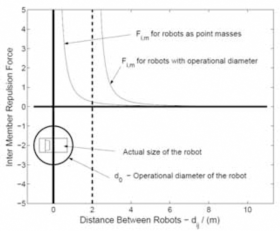
Physical Size of Robots : For the general case we consider the swarm consists of members with physical dimensions, length (l
m
) and width (w
m
). Let l
m
> w
m
, then we define the operational diameter of a robot (d
v
) as d
o
= k
o
× l
m
(refer Fig. 4.); where k
o
> 1 is considered as the safety factor for collision avoidance (similar to safety factor in mechanical/structural designs; k
o
can be chosen to suite the maximum speed of motion and to adjust the clearance level). Then the modified artificial force for inter-member repulsion is as follows:


Car like robots with operational diameter
where d ij = (αX i − αX j ).
Comparison of
Comparison of
Chattering Effect: As discussed in the section 2.3, chattering effects due to the decreasing nature of the attraction force become a significant issue when a large number of robots are operating at low speeds. Lower momentum of the robots and higher F
i,m
forces prevent some member from entering the shape. This problem can successfully be eliminated by modifying the F
i,a
force as expressed in (40). In the modified function, an additional term is included which increases the attraction force as the member is approaching the contour. Also this addition improves the uniformity of the “Artificial Formation Forces” in either side of the contour.
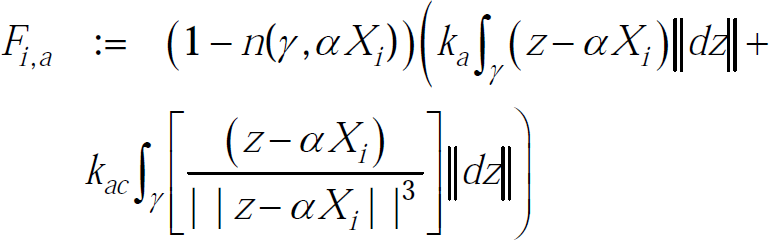
In the above expression k ac is the weighing parameter of the force component which dominates when the member is closer to the contour.
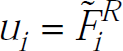
Actuator Limitations: Next, we modify the force function to eliminate the problem of unrealistic accelerations, by introducing maximum force parameters into the resultant force function. The controller (u
i
) with modified force function is as follows,
where,
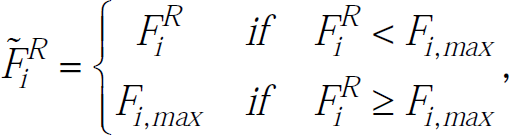
in which
Since the mechanical limitations and road/safety limits control the maximum speed that a mobile agent (e.g. ground vehicles traveling in rough terrains can achieve a maximum speed of about 120km/h), we introduce a velocity limiting function as follows,

Here the term v
max
represents maximum velocity that the mobile agent can achieve.
The shape formation algorithm, ideally suited for outdoor deployment of a group of mobile robots, has two basic implementation stages; initial parameter selection (design) and deployment. Prior to the deployment, the target contours, obstacle contours are to be clearly defined and the corresponding contour functions relative to the robot coordinate system (e.g. GPS) are to be generated. Considering the weighing parameters of the artificial force functions (i.e. k m ,k f ,k r etc.), the proper parameters have to be selected depending on the application and the constrains provided in the analysis sections. The next stage is to deploy the mobile agents programmed with designed contours and parameters. Indeed, the algorithm provides provisions to change the contour functions and parameters, and to add/remove agents in an already deployed group. But this needs effective communication between control center and the group. The behavior of the swarm for such situations are presented in the simulation section.
Remark
In the pre-deployment stage, the target and obstacles can effectively be identified using satellite maps. Also if we consider a military type deployment, the intelligence sources such as real-time satellite coverage, aerial video updated from UAV's etc, can be used to determine new obstacles, ‘no entry’ zones etc, for dynamic parameter modification of the robot group.
For successful implementation of the shape formation algorithm the ideal mobile robots need the following capabilities;
Instantaneous and error free self localization. Knowledge of location of all other members of the group without delay. (using communication network)
Here we discuss the practical implementation issues and some technologies which provide near ideal capabilities to the robots.
Since we are mainly focusing on outdoor applications with this algorithm, self localization of robots can use Global Positioning System (GPS) technology. With modern developments in P-Code GPS receivers less than 5m horizontal accuracies can be achieved. And with Differential GPS technology, where a reference base station (a DGPS base station can be used effectively within 100 km range) is used to cancel out the atmospheric and data transmission errors, providing sub-meter accuracies (Bajaj, Ranaweera et al. 2002; http://www.Trimble.com) even for C/A Code civilian GPS receivers with instantaneous (1Hz) position updates. Further, recent advances in commercial GPS receivers an accuracy range within 1cm could be achieved, although this introduces an acquisition delay (typically 45min) thus suited for slow moving applications requiring higher accuracies.
Next we discuss the GPS localization errors. Due to delays in update rates, there will be positional errors when the agent is moving at a significant speed. For example, if the GPS receiver updates the position in 1Hz frequency, a robotic vehicle moving in 4m/s can have 4m error due to the motion. But, using inertial navigating technologies, in which acceleration is used to calculate positions, together with GPS technology the short range errors in GPS can be eliminated (Caldwell 1988; Gamble and Jenkins 2000; Hyslop, Gerth et al. 1990; Loffler and Nielson 2003; Renfroe, McMinemon et al. 2000) leaving only the random measurement noise as errors.
In conclusion, the self localization of the mobile robots can be achieved to a desirable level, in which the error can be modeled as follows;
where
Positional information of members is a crucial aspect in the shape formation algorithm. This location information is sent through a wireless RF links (or communication network). The ability to communicate with each other at the same time can be restrictive in real world applications. Even with the CDMA technology (Schiller 2003) to communicate with many devices at once, due to high degree of interferences, the effectiveness of the communication will degrade with increasing number of members of the group. The interferences can be minimized using transmission power control, although it reduces the range of transmission. Wireless mesh networking technology (Bruno, Conti et al. 2005; Lee, Zheng et al. 2006) can be a better solution since it enables to handle larger data flows with increased number of nodes (Jun and Sichitiu 2003). However delays in data transmission (due to routing) and range limitations (Hincapie, Sierra et al. 2007) are common problems in mesh networks. Thus we can only achieve the instant communication capabilities within a certain radius from a robot, and the modified inter-member repulsion force can be given as follows;

where
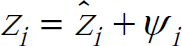
Here d c refers to the radius that a robot can transmit a signal without interfering with other communications within the group or in other words “effective range of communication”. For example, in the platoon of vehicles shown in Fig. 6., the vehicle A will have the position information of B,C,D and E; which are in close proximity to A.
Robots navigate using restricted inter-member force due to limited communication range.
Remark
The same artificial force as above can be used to model communication failures. In such situations the dc become the range of the sonar/laser range and bearing finders which serve as backup devices to eliminate inter-member collisions.
The swarm shape formation algorithm and the controller behavior is simulated for two basic cases; with ideal conditions and under certain restrictions in the real world scenario. The controller used for the first set of cases has the basic swarm model introduced in (7). For the second set of cases, we used the modified controller components presented in the previous section. The main objective of these simulation case studies is to investigate the behavior of the swarm in relevant potential situations.
Remark
In the simulations, the shape contour was generated by the mathematical function described in Appendix I. Also the artificial friction force weighing parameter is selected such that
Ideal Environment and Conditions
The simulation for ideal conditions are basically to demonstrate the shape formation algorithm and to evaluate some theoretical assertions presented in the previous sections. Initially, we demonstrate the behavior of the swarm in forming into different shapes using four cases. Next we present the swarming behavior and the validity of the “X Swarm” hypothesis. Here the assertions proved in theorems 1 and 2 are demonstrated using a visual representation. Finally we present the cases where the swarm is subjected to sudden change in the shape, loss of members and addition of new members.
Shape Formation
The motion/behavior of the swarm is demonstrated for four cases; in all sub figures in Fig. 7., crosses represent initial positions and the dots represent final positions (after 100s) while the motion paths are represented by thin lines. In Fig. 7.(a) we demonstrate the motion of the swarm initially in a line formation and in the Fig. 7.(b), (c) and (d) the initial positions of the members are randomly selected. From these four cases it is evident that the swarm converges to the desired shape and distributes evenly, regardless of the initial positions, size of the swarm and the size/shape of the contour, provided that the necessary parameters are carefully selected. The shape generation parameters and the number of robots used in the four cases are listed in Table 1. For these simulations the weighing parameters were selected as : k a = 4 × 10⁻³, k r = 5 × 10³ and k m = 6 × 10⁶.

Motion of the swarm to generate different shapes
Parameters in shape generation

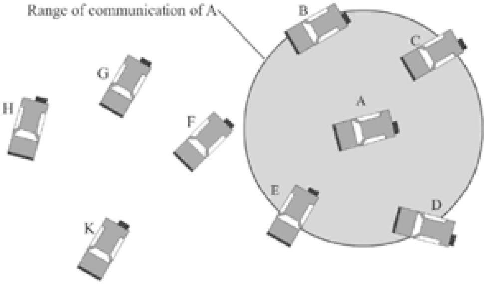
In this section we demonstrate the validity of the “X Swarm” hypothesis in a simulated swarm, evaluating our results presented in theorems 1 and 2, i.e. motion of the center of mass of the swarm and the motion of an individual outside the swarm. Theorem 1 does not impose any restriction for convergence other than the selection of k
f
for stability. According to theorem 2, for a member of a “X Swarm”, staying outside the shape while satisfying
Swarm motion and “X Swarm” hypothesis, for (δ + Δ) > 82m and N = 14.
Note that the center error rapidly decrease while the members are outside the shape, demonstrating the behavior predicted by theorem 1 and after moving into the shape we can observe a slow convergence. Fig. 8.(c) and (d) illustrate the behavior of member error (v) for three selected members and the average error. We have intentionally chosen the parameters such that “X Swarm” behavior is achieved only for a certain period. The regions “A” and “B” represents the time spans where “X Swarm” hypothesis is valid. Note that since the swarm expands after it reaches the shape, the “X Swarm” hypothesis is valid for all t > 100. In the zoomed view of the member error (Fig 8.(d)), one can notice that the members converge toward the center of mass of the swarm despite the invalidity of the “X Swarm” hypothesis and even after the member enters the shape.
Also from the figures it can be noticed that member error continuously decreases when the member is outside the shape and the swarm behaves as a “X Swarm”, demonstrating the validity of the assertions presented in Theorem 2. For this simulation we used the following parameters for shape generation: a=5, b=1, c=0.5 and d=80. The weighing parameters for the controller were selected as : k a = 7 × 10⁻³, k r = 5 × 10³ and k m = 6 × 10⁶.
Here we demonstrate the behavior of the swarm, when subjected to a sudden change in the contour shape. This kind of shape transitions are important in real world applications, specially in weapon deployment systems as presented in (Ekanayake and Pathirana 2007; Ekanayake and Pathirana 2008). From the computer simulation results Fig. 9. shows the initial positions of the swarm. In the Fig. 10., the motion paths of members and final positions after forming into the new shape is depicted. It is clear from this simulation, the members effectively maneuver themselves to form the new shape and redistribute themselves within that shape. The simulation used the parameters in Table 2. For this simulation we selected the weighing parameters for the controller as : k a = 4 × 10⁻³, k r = 5 × 10³ and k m = 6 × 10⁶.

Shape transition - initial positions of the swarm (@ t=0)

Shape transition - positions after reforming into the new shape (@ t=50)
Parameters in shape generation

Addition and removal of agents from a deployed swarm can be due to several reasons. In most applications, swarm robots are deployed in highly hostile environments (e.g. battle fields, de-mining, underwater data collection etc) which results in frequent failures in the robots and some times, loss of robots. In such circumstances the existing robots should re-organize (or redistribute) to cover the whole area of the target until reinforcements arrive, and once the reinforcements (or substitutes) arrived they should reorganize once again to include new members into the shape. In the simulation case studies presented in Fig. 11. and Fig. 12., we illustrate the behavior of the swarm upon removal of members and after the arrival of new members respectively. For the shape generation we used the parameters listed in Table 3. The weighing parameters for the controller were selected as : k a = 4times10−3, k r = 5times103 and k m = 6times106.
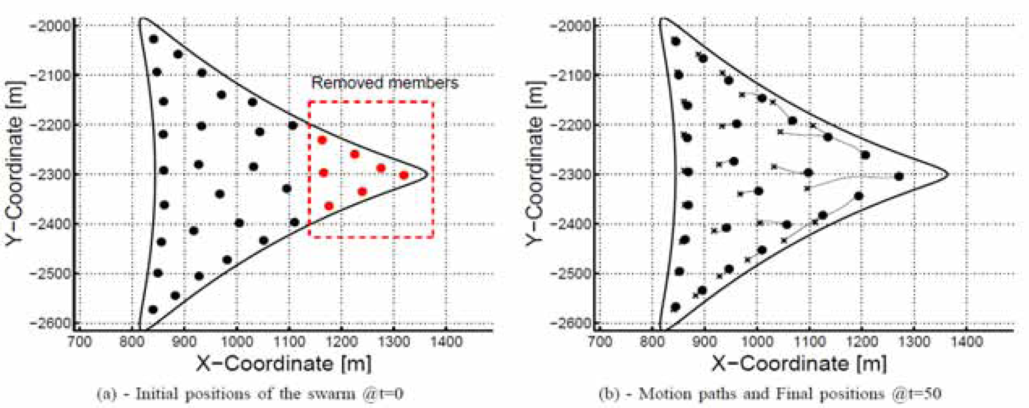
Swarm behavior when a set of members removed from the swarm. (The red dots in (a) represent the member to be removed at t=0.)

Swarm behavior to include new members to the shape. (The red dots represent newly added members and the red lines represents their motion paths)
Parameters in shape generation

For the case studies presented in this section we simulate some real world scenarios and the behavior of the swarm in such situations. For all the simulations in this section we include velocity and actuator limitations, such that the velocity is limited to 30m / s and acceleration is limited to 0.5G (4.9m/s2). Also the k ac parameter (weighing parameter for close range attraction force) is selected as same as the k r in each case.
Obstacle Avoidance
Two cases are presented and in the first case (Fig. 13.(a)) the vehicles (mobile robots) are in a line formation (for example along a road or in a convoy) and the target contour is located beyond two obstacle contours. As illustrated in the figure, the mobile robots successfully avoid both obstacles and form the desired shape by t = 1000s.
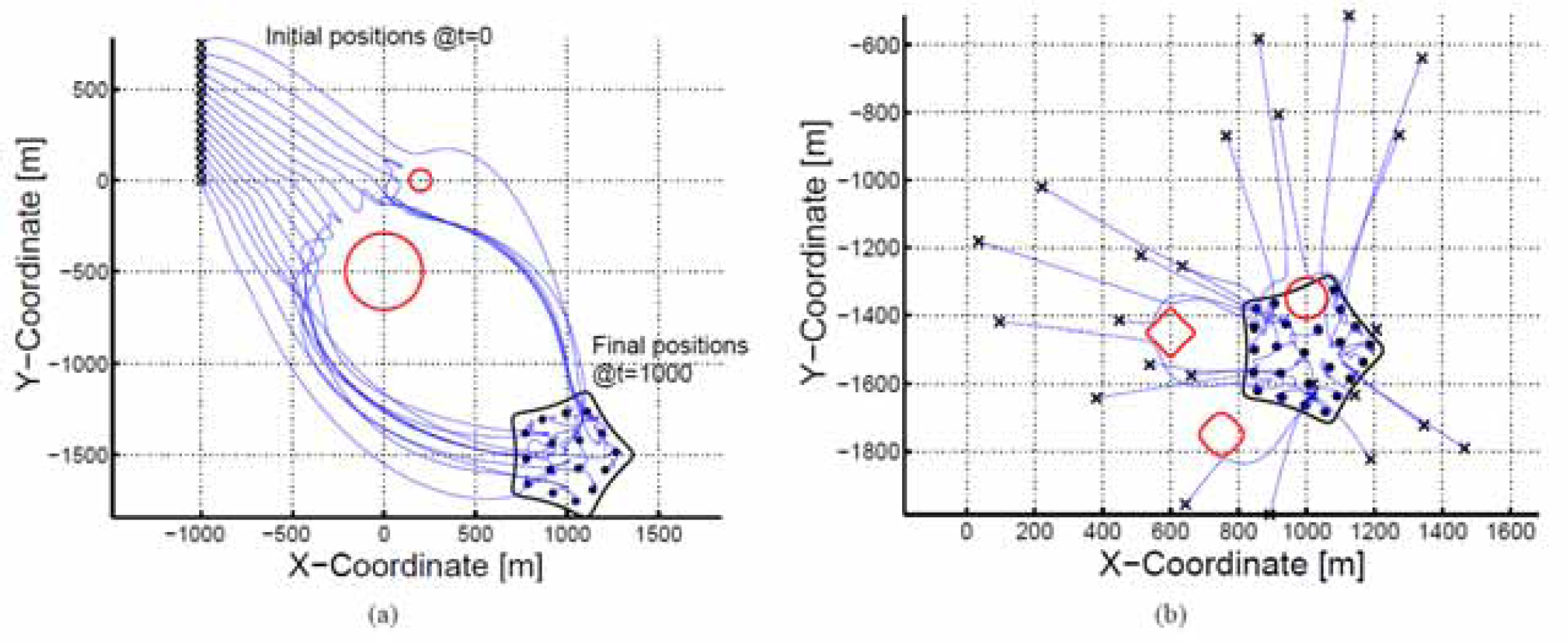
Motion of the swarm in presence obstacles
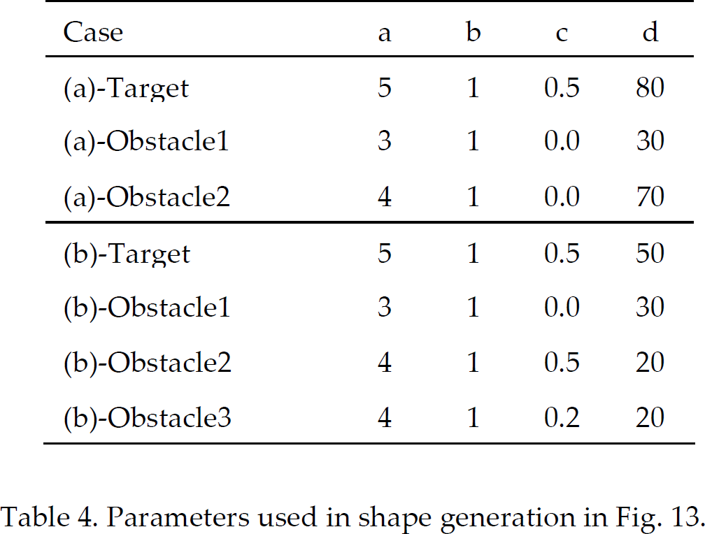
Parameters used in shape generation in Fig. 13.
Weighing parameters for artificial forces (Fig. 13)

In the second case, we consider a situation where mobile robots are randomly distributed around the target contour. Here we used two obstacles outside the target contour and one obstacle inside the target. Here also the mobile robots successfully maneuvered around the obstacles and moved into the desired shape. (The parameters listed in Table 4 an 5 were used for this simulation case.)
Assuming technologies and mathematical representations in section 3; the agent size compensation, localization errors and communication limitations are modeled using equations (44) and (45). In figures 14.(a) and 14.(b) we present the swarm behavior with real-world conditions (i.e. all the above included) and with ideal conditions respectively. In both cases, the weighing parameters for artificial forces and shape parameters are kept the same. The effective range of communication of 150m and a random localization error up to 5m are used in simulating non ideal effects. When comparing the two cases, no significant difference could be observed in the final formation, other than the more uniform distribution in the latter case. This is due to low F i,m component since communication limitations do not permit inclusion of all the members in determining that force.

Motion of the swarm in a real-world environment
In this paper, we presented an approach for formation of shapes for a swarm, which has many potential real-world applications. The stability of convergence, prospective stable points inside a given symmetric shape, have been analyzed; the effectiveness of the aggregation, theoretical assertions were confirmed using computer simulations. Also we ensure that the shape formation algorithm can effectively be used in real world applications using simulation case studies which models the constraints and errors encountered in real world scenarios.
Our approach of shape formation without nominating specific locations to each member, ensures that the shape/area of interest is completely covered by the swarm. This makes our algorithm applicable in many defense, land/space exploration systems.
Although, this algorithm can be used with non symmetric contours, the explicit stability point(s) inside such a contour is left for future work. This formation algorithm is easily extendable to complex contours that consists of several closed simple contours.
Appendix I - Mathematical Function for Contour Generation
For the simulation of the algorithm, the contour γ s are generated by a mathematical function in the following form,

The properties of the function varies with a,b,c and d as follows, i.e. parameter a ∈ determines the number of edges in the contour. Parameter b = 1 for a simple closed contour and c determines the smoothness of the edges (c > 1 makes the edges to wind, c = 1 makes sharp edges and c < 1 results in round edges with c = 0 making a circle). Parameter d > 0 determines the overall size of the shape.
