Sage Journals: Discover world-class research

Abstract

This article examines the static area coverage problem by a network of mobile, sensor-equipped agents with imprecise localization. Each agent has uniform radial sensing ability and is governed by first-order kinodynamics. To partition the region of interest, a novel partitioning scheme, the Additively Weighted Guaranteed Voronoi diagram is introduced which takes into account both the agents’ positioning uncertainty and their heterogeneous sensing performance. Each agent’s region of responsibility corresponds to its Additively Weighted Guaranteed Voronoi cell, bounded by hyperbolic arcs. An appropriate gradient ascent-based control scheme is derived so that it guarantees monotonic increase of a coverage objective and is extended with collision avoidance properties. Additionally, a computationally efficient simplified control scheme is offered that is able to achieve comparable performance. Several simulation studies are offered to evaluate the performance of the two control schemes. Finally, two experiments using small differential drive-like robots and an ultra-wideband positioning system were conducted, highlighting the performance of the proposed control scheme in a real world scenario.

Keywords

Multi-agent systems multi-robot systems mobile robots cooperative systems autonomous agents

Introduction

Area coverage of a planar region by a swarm of robotic agents is an active field of research with great interest and potential. The task involves the dispersal inside a region of interest of autonomous, sensor-equipped robotic agents to achieve sensor coverage of that region. Some of the possible applications for multi-agent coverage are environmental and crop monitoring, search and rescue or surveillance.¹ Distributed control algorithms are a popular choice for this task because of their computational efficiency compared to centralized controllers, their ability to adapt in real time to changes in the robot swarm and their reliance only on local information. Thus they can be implemented on robots with low computational power and low power radio transceivers since each agent is required to communicate only with its neighbors. The downside of distributed control schemes is that they lead to local optima of their objective function because of the lack of information on the state of all agents.

Area coverage can be categorized either as static^2,3 in which case the goal is the convergence of the agents to some static final configuration or sweep^4,5 in which the agents continuously move inside the region of interest in order to satisfy some changing coverage objective.

Other factors that affect the choice of control scheme are the dynamics of the agents used,^6,7 the geometrical characteristics of the region of interest,^8,9 and the sensing performance of the agents’ sensors.^10,11

Several varying approaches to the coverage problem have been proposed, including annealing algorithms,¹² game theory,¹³ distributed optimization,¹⁴ model predictive control,^15,16 optimal control,¹⁷ and event-triggered control.¹⁸

Due to the inherent uncertainty in the measurements of all localization systems, there is great interest in incorporating this uncertain information in the control scheme. There have been approaches such as the use of probabilistic methods,¹⁹ data fusion²⁰ or safe trajectory planning.²¹ In this article, we use a Voronoi-like partitioning scheme that takes into account the agents’ positioning uncertainty and design a suitable gradient-based control law to solve the area coverage problem. Other partitioning schemes based on Voronoi diagrams have been proposed for collision avoidance with static obstacles²² and between mobile agents.²³

The problem of static area coverage of a convex planar region of interest by a network of heterogeneous agents is examined in this article. The agents are equipped with isotropic sensors whose performance is allowed to differ among agents, resulting in a heterogeneous team with respect to each agent’s sensing performance. The goal of the agent team is achieving coverage over as large part of the region of interest as possible in a cooperative manner using their on-board sensors. The localization uncertainty is taken into account by assuming that each agent resides somewhere within a circular positioning uncertainty region. These uncertainty regions along with the agents’ sensed regions are used to create an Additively Weighted Guaranteed Voronoi (AWGV) partitioning of the region of interest and subsequently, a gradient-based distributed control law is derived. The control law guarantees the monotonic increase of an area coverage objective. This control law is then extended with a collision avoidance scheme to ensure the safe operation of agents. A computationally efficient simplified control law is also presented. Both control schemes are evaluated through simulation studies. Moreover, experimental results are presented to provide a complete overview of the proposed control scheme. This article is an extension of the work by Papatheodorou et al., ^24,25 which did not account for heterogeneous agents, implemented only the simplified control law, and did not provide collision avoidance guarantees. The main contribution of this article is the incorporation of the agents’ localization uncertainty in the coverage control scheme by introducing the AWGV diagram and presenting an experimental implementation of the devised control scheme.

Mathematical preliminaries

Assume a compact convex region $Ω \in ℝ^{2}$ under surveillance and a network of n dimensionless mobile agents. Each agent’s dynamics is governed by

{\dot{q}}_{i} = u_{i}, q_{i} \in Ω, u_{i} \in ℝ^{2}, i \in I_{n}

where u_i is the control input for each agent and $I_{n} = {1, 2, \dots, n}$ .

The agents’ positions are not known precisely and thus in the general case each agent has a positioning uncertainty of different measure. We assume that an upper bound r_i for the positioning uncertainty of each agent is known and thus its center resides within a disk

C_{i}^{u} (q_{i}, r_{i}) = {q \in Ω : ∥ q - q_{i} ∥ \leq r_{i}}, i \in I_{n}

where ∥⋅∥ is the Euclidean metric and q_i the agent’s position as reported by its localization equipment.

All agents are equipped with omnidirectional sensors with circular sensing footprints and as such the sensed region of each agent can be defined as

C_{i}^{s} (q_{i}, R_{i}) = {q \in Ω : ∥ q - q_{i} ∥ \leq R_{i}}, i \in I_{n}

where R_i is the sensing range of each sensor.

We also define for each agent a “Guaranteed Sensed Region” (GSR) as the region that is sensed by the agent for all of its possible positions inside $C_{i}^{u}$ . The GSRs are defined as

C_{i}^{g s} (C_{i}^{u}, C_{i}^{s}) = {\underset{q_{i}}{\cap} C_{i}^{s} (q_{i}, R_{i}), \forall q_{i} \in C_{i}^{u}}, i \in I_{n}

and since $C_{i}^{u}$ and $C_{i}^{s}$ are disks, the previous expression can be further simplified into

C_{i}^{g s} (q_{i}, R_{i}^{g}) = {q \in Ω : ∥ q - q_{i} ∥ \leq R_{i}^{g}}, i \in I_{n}

where $R_{i}^{g} = R_{i} - r_{i}$ , provided that $R_{i} \geq r_{i}$ .

When an agent’s position is known precisely, that is, $r_{i} = 0$ , its GSR is equivalent to its sensed region, whereas when an agent’s positioning uncertainty is too large compared to its sensing capabilities, that is, $r_{i} > R_{i}$ , then $C_{i}^{g s} = \emptyset$ .

Space partitioning

Most distributed area coverage schemes assign an area of responsibility to each agent using a Voronoi or Voronoi-inspired partitioning scheme. In this article, due of the localization uncertainty of the agents as well as their heterogeneous sensing patterns, the AWGV diagram described in section “AWGV diagram” section is developed for the assignment of areas of responsibility.

Guaranteed Voronoi diagram

The GV diagram²⁶ is defined for a set of uncertain regions $D = {D_{1}, D_{2}, \dots, D_{n}}, D_{i} \subset Ω$ . Each uncertain region D_i contains all possible positions of a point $q_{i} \in ℝ^{2}$ whose localization cannot be measured precisely. The GV diagram generates cells W_i, defined as

\begin{array}{l} W_{i} = {q \in Ω : max ‖ q - q_{i} ‖ \leq min ‖ q - q_{j} ‖ \\ \forall j \in I_{n}, j \neq i, q_{i} \in D_{i}, q_{j} \in D_{j}}, i \in I_{n} \end{array}

Each cell W_i contains the points on the plane that are closer to the corresponding point q_i of region D_i for all possible configurations of the uncertain points. It is important to note that when two or more uncertain regions overlap, none of them are assigned GV cells. In addition, if the uncertain regions degenerate into points, the GV diagram converges to the classic Voronoi diagram.

Remark 1

In contrast to the classic Voronoi diagram, the GV diagram does not constitute a tessellation of Ω, since $\cup_{i \in I_{n}} W_{i} \subset Ω$ .

AWGV diagram

The AWGV diagram is a generalization of the GV diagram in which each uncertain region is assigned an importance weight, similarly to the Additively Weighted Voronoi diagram.^27

–30 Uncertain regions with greater weights are assigned larger portions of the region Ω. Using the agents’ guaranteed sensing radii $R_{i}^{g}$ as weights, it is possible to assign them regions of responsibility based on their sensing performance as well as their positioning uncertainty. The AWGV diagram for a set of uncertain regions $D = {D_{1}, D_{2}, \dots, D_{n}}, D_{i} \subset Ω$ with weights $R = {R_{1}^{g}, R_{2}^{g}, \dots, R_{n}^{g}}, R_{i}^{g} \in ℝ$ is defined as

\begin{array}{l} W_{i}^{g} = {q \in Ω : max ‖ q - q_{i} ‖ - R_{i}^{g} \leq min ‖ q - q_{j} ‖ - R_{j}^{g} \\ \forall j \in I_{n}, j \neq i, q_{i} \in D_{i}, q_{j} \in D_{j}}, i \in I_{n} \end{array}

As such, each cell $W_{i}^{g}$ contains the points on the plane that are closer to the corresponding weighted point q_i of region D_i for all possible configurations of the uncertain points. In contrast to the GV diagram, when two or more uncertain regions overlap, it is possible that the one with the largest weight is assigned an AWGV cell. It can be shown that if the weights are equal, the AWGV converges to the GV diagram. Moreover, if the uncertain regions degenerate into points, the AWGV diagram converges to the additively weighted Voronoi diagram and if in addition to that the weights are equal, then it converges to the classic Voronoi diagram.

Remark 2

Similar to the GV diagram, the AWGV diagram does not constitute a tessellation of Ω, since $\cup_{i \in I_{n}} W_{i}^{g} \subset Ω$ . We define a neutral region $O$ so that $O \cup \cup_{i \in I_{n}} W_{i}^{g} = Ω$ .

It is useful to define the R-limited AWGV cells as

W_{i}^{R} = W_{i}^{g} \cap C_{i}^{g s}, i \in I_{n}

which are the parts of the AWGV cells that are guaranteed to be sensed by their respective agents. It can be shown that since AWGV cells are disjoint, these R-limited cells are also disjoint regions.

AWGV diagram of disks

Given the fact that the uncertain regions have been assumed to be disks $C^{u} = {C_{1}^{u}, C_{2}^{u}, \dots, C_{n}^{u}}, C_{i}^{u} \subset Ω$ , the definition of the AWGV diagram can be simplified into

\begin{array}{l} W_{i}^{g} = {q \in Ω : ‖ q - q_{i} ‖ + r_{i} - R_{i}^{g} \leq ‖ q - q_{j} ‖ - r_{j} - R_{j}^{g}, \\ \forall j \in I_{n}, j \neq i}, i \in I_{n} \end{array}

An equivalent definition is

W_{i}^{g} = Ω \cap \underset{j \in I_{n} \ i}{\cap} H_{i j}

where

\begin{matrix} H_{i j} = {q \in Ω : ‖ q - q_{i} ‖ + r_{i} - R_{i}^{g} \leq ‖ q - q_{j} ‖ - r_{j} - R_{j}^{g}} \\ = {q \in Ω : ‖ q - q_{j} ‖ - ‖ q - q_{i} ‖ \geq + r_{i} + r_{j} - R_{i}^{g} + R_{j}^{g}} \end{matrix}

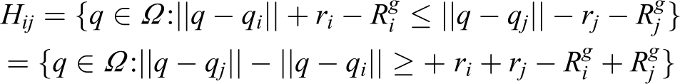
Thus, the boundary $\partial H_{i j}$ is given by

\partial H_{i j} = {q \in Ω : ‖ q - q_{j} ‖ - ‖ q - q_{i} ‖ = r_{i} + r_{j} - R_{i}^{g} + R_{j}^{g}}

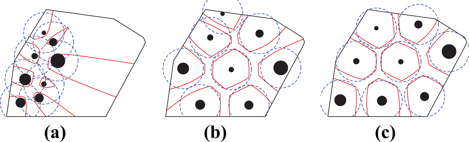
which is the equation of one branch of a hyperbola with foci at q_i and q_j and semi-major axis $a_{i j} = \frac{r_{i} + r_{j} - R_{i}^{g} + R_{j}^{g}}{2}$ . Since $a_{i j}$ can be either positive or negative, $\partial H_{i j}$ will correspond to the “East” or “West” branch of a hyperbola respectively, thus the region $H_{i j}$ can be either convex or non-convex, respectively.

Figure 1 shows the change in the AWGV cells of two agents as the sensing radius of the $i th$ agent decreases. The uncertainty regions are shown as filled disks, the sensing regions as dashed circles, and the boundaries of the AWGV cells as well as the region Ω are shown in solid lines. The cell, uncertainty, and sensing region of agent i are shown in blue, while those of agent j are shown in red and the region Ω in black. In Figure 1(a), agent i has been assigned the whole region, while the cell of agent j is empty. In Figure 1(b) and (c), the cell of agent i is non-convex, while that of agent j is convex. As the sensing radius of agent i decreases, the area of its cell decreases, while the area of the cell of agent j increases. In Figure 1(d), the cell of agent i is bounded by a straight line because $a_{i j} = 0$ . Figure 2 shows a comparison between the classic Voronoi, the GV, and the AWGV diagrams. The agent positions and uncertainty regions are represented by black disks, their respective cells in red and their sensing regions in dashed black lines.

Figure 1.

AWGV cells as the sensing radius of the ith agent decreases. AWGV: Additively Weighted Guaranteed Voronoi.

Figure 2.

Comparison of partitioning schemes: (a) classic Voronoi, (b) GV, and (c) AWGV. AWGV: Additively Weighted Guaranteed Voronoi.

Remark 3

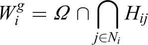
We define the AWGV neighbors N_i of an agent i with respect to the AWGV partitioning as those agents that are required to construct the AWGV cell of agent i. These are defined as

N_{i} = {j \in I_{n}, j \neq i : \partial H_{i j} \cap \partial W_{i}^{g} \neq \emptyset}

Thus, the cell of agent i can be written as

W_{i}^{g} = Ω \cap \underset{j \in N_{i}}{\cap} H_{i j}

Problem statement – distributed control law

By taking into account the AWGV partitioning of the space, the following area coverage criterion is constructed

\begin{matrix} H = \int_{\underset{i \in I_{n}}{\cup} W_{i}^{R}} ϕ (q) d q \\ = \sum_{i \in I_{n}} \int_{W_{i}^{R}} ϕ (q) d q = \sum_{i \in I_{n}} H_{i} \end{matrix}

where the function $ϕ : ℝ^{2} \to ℝ_{+}$ is related to the a priori knowledge of importance of a point $q \in Ω$ , indicating the probability of an event to take place at q in a coverage scenario. This criterion expresses the area that is guaranteed to be closest to and covered by the agents.

A distributed control law is designed to maximize the coverage criterion (9), while taking into account the agents’ guaranteed sensing pattern in equation (3) and the AWGV partitioning equation (7). It is shown that this control law leads to a monotonic increase of the coverage criterion.

Theorem 1

For a network of mobile agents with uncertain localization as in equation (2), uniform range-limited radial sensing performance as in equation (3), governed by the individual agent’s kinodynamics described in equation (1), and the AWGV partitioning of Ω defined in equation (7), the coordination scheme

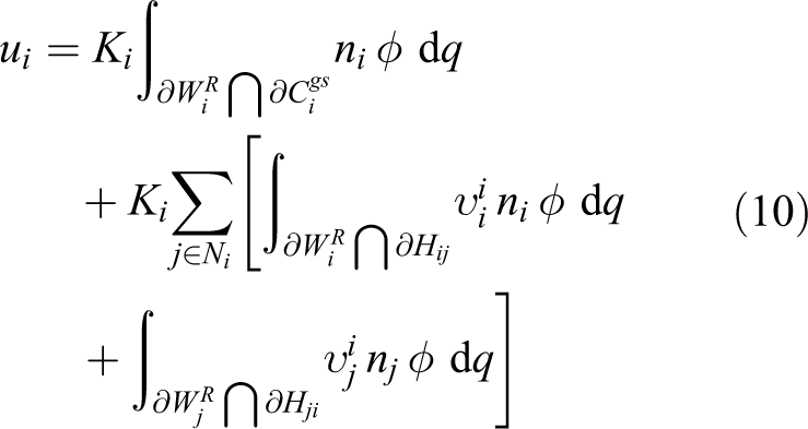
$\begin{matrix} u_{i} = K_{i} \int_{\partial W_{i}^{R} \cap \partial C_{i}^{g s}} n_{i} ϕ d q \\ + K_{i} \sum_{j \in N_{i}} [\int_{\partial W_{i}^{R} \cap \partial H_{i j}} υ_{i}^{i} n_{i} ϕ d q \\ + \int_{\partial W_{j}^{R} \cap \partial H_{j i}} υ_{j}^{i} n_{j} ϕ d q] \end{matrix}$
10

where n_i is the outward unit normal on $\partial W_{i}^{R}$ and K_i a positive constant, maximizes the performance criterion (9) along the agents’ trajectories in a monotonic manner, leading to a locally area-optimal configuration of the network.

Proof

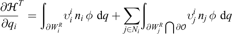
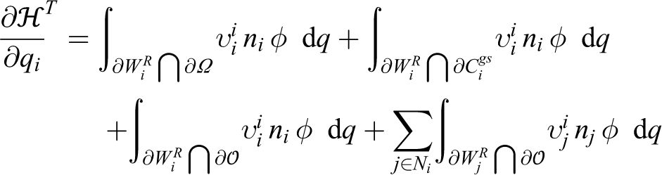
In order to guarantee monotonic increase of the coverage criterion (9), we evaluate its time derivative

$\frac{d H}{d t} = \sum_{i \in I_{n}} \frac{\partial H_{i}}{\partial q_{i}} {\dot{q}}_{i} = \sum_{i \in I_{n}} \frac{\partial H_{i}}{\partial q_{i}} u_{i}$

Using the gradient-based control law

$u_{i} = K_{i} {\frac{\partial H_{i}}{\partial q_{i}}}^{T}, i \in I_{n}$

where $K_{i} > 0$ , monotonic increase of $H$ is achieved.

We now evaluate the partial derivative of $H$ with respect to q_i as

$\frac{\partial H}{\partial q_{i}} = \frac{\partial}{\partial q_{i}} \int_{W_{i}^{R}} ϕ d q + \sum_{j \in N_{i}} \frac{\partial}{\partial q_{i}} \int_{W_{j}^{R}} ϕ d q$

Considering the second summation term, infinitesimal motion of q_i may only affect $\partial W_{j}^{R}$ at $\partial W_{j}^{R} \cap \partial O$ , where $O$ is the neutral region defined in remark 2, since both hyperbola branches are affected by alteration of one of the foci. In addition, only the AWGV neighbors (equation (8)) of the ith agent are considered in the summation, as a major property of AWGV-partitioning. Therefore, the former expression can be written via the generalized Leibniz integral rule³¹ (by converting surface integrals to line ones) as

${\frac{\partial H}{\partial q_{i}}}^{T} = \int_{\partial W_{i}^{R}} υ_{i}^{i} n_{i} ϕ d q + \sum_{j \in N_{i}} \int_{\partial W_{j}^{R} \cap \partial O} υ_{j}^{i} n_{j} ϕ d q$

where $υ_{i}^{i}, υ_{j}^{i}$ stand for the transpose Jacobian matrices with respect to q_i of the points $q \in \partial W_{i}^{R}$ , $q \in \partial W_{j}^{R}$ , respectively, that is,

$υ_{j}^{i} (q) ≜ {\frac{\partial q}{\partial q_{i}}}^{T}, q \in \partial W_{j}^{R}, i, j \in I_{n}$
11

The boundary $\partial W_{i}^{R}$ can be decomposed in disjoint sets as

$\begin{array}{l} \partial W_{i}^{R} = {\partial W_{i}^{R} \cap \partial Ω} \cup {\partial W_{i}^{R} \cap \partial C_{i}^{g s}} \\ \cup {\partial W_{i}^{R} \cap \partial O} \end{array}$
12

These sets represent the parts of $\partial W_{i}^{R}$ that lie on the boundary of Ω, the boundary of the agent’s GSR, and the boundary of the unassigned neutral region of Ω, respectively. This decomposition is shown in Figure 3 with $\partial W_{i}^{R} \cap \partial Ω$ in green, $\partial W_{i}^{R} \cap \partial C_{i}^{g s}$ in solid red, and $\partial W_{i}^{R} \cap \partial O$ in solid blue.

Figure 3.
Decomposition of $\partial W_{i}^{R}$ into disjoint sets.

Hence ${\frac{\partial H}{\partial q_{i}}}^{T}$ can be written as

$\begin{array}{l} {\frac{\partial H}{\partial q_{i}}}^{T} = \int_{\partial W_{i}^{R} \cap \partial Ω} υ_{i}^{i} n_{i} ϕ d q + \int_{\partial W_{i}^{R} \cap \partial C_{i}^{g s}} υ_{i}^{i} n_{i} ϕ d q \\ + \int_{\partial W_{i}^{R} \cap \partial O} υ_{i}^{i} n_{i} ϕ d q + \sum_{j \in N_{i}} \int_{\partial W_{j}^{R} \cap \partial O} υ_{j}^{i} n_{j} ϕ d q \end{array}$

It is apparent that $υ_{i}^{i} = 0$ at $q \in \partial W_{i}^{R} \cap Ω$ since all $q \in \partial Ω$ remain unaltered by infinitesimal motions of q_i, assuming no alteration of the environment. Considering the second integral, for any point $q \in \partial W_{i}^{R} \cap \partial C_{i}^{g s}$ it holds that $υ_{i}^{i} (q) = I_{2}$ , where $I$ stands for the identity matrix, since they translate along the direction of motion of q_i at the same rate. As far as the sets $\partial W_{i}^{R} \cap \partial O$ and $\partial W_{j}^{R} \cap \partial O, j \in N_{i}$ are concerned, they can be merged in pairs via utilization of the left and right hyperbolic branches, as introduced in AWGV-partitioning (equation (7)), as follows

$\begin{matrix} {\frac{\partial H}{\partial q_{i}}}^{T} = \int_{\partial W_{i}^{R} \cap \partial C_{i}^{g s}} n_{i} ϕ d q \\ + \sum_{j \in N_{i}} [\int_{\partial W_{i}^{R} \cap \partial H_{i j}} υ_{i}^{i} n_{i} ϕ d q \\ + \int_{\partial W_{j}^{R} \cap \partial H_{j i}} υ_{j}^{i} n_{j} ϕ d q] \end{matrix}$
13

The unit normal vectors $n_{i}, n_{j}$ and Jacobian matrices $υ_{i}^{i}, υ_{j}^{i}$ in the second part of equation (13) can be evaluated via utilization of the parametric representations of the sets over which the integration takes place. These sets are parts of the branches of a hyperbola ( $\partial H_{i j}$ and $\partial H_{j i}$ ) that assigns the space among two arbitrary agents $i, j$ . The evaluation of the normal vectors and Jacobian matrices is examined in more detail in the Appendix 1.

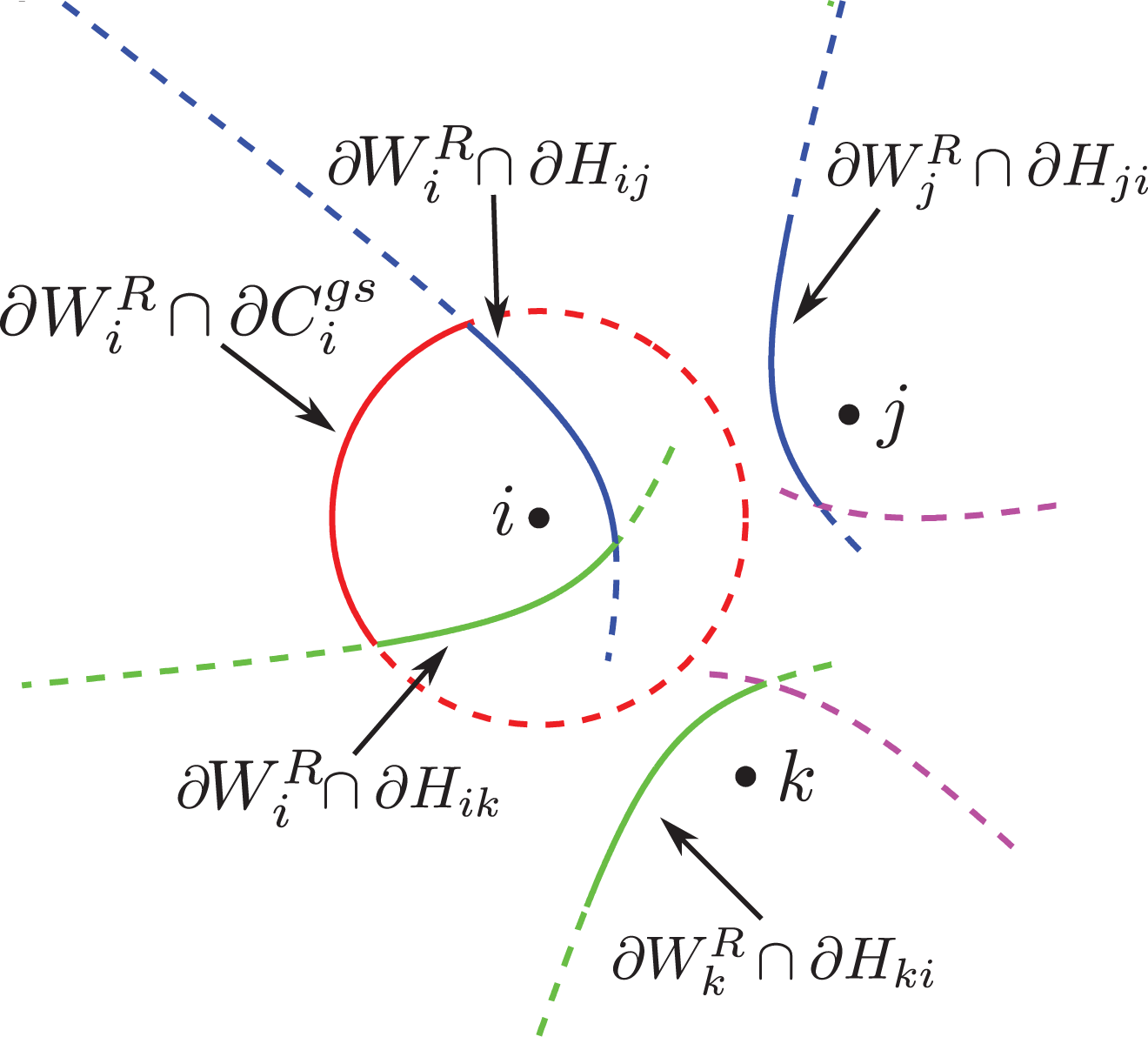
The decomposition of the set $\partial W_{i}^{R} \cap \partial O$ of agent i into mutually disjoint hyperbolic arcs $\partial W_{i}^{R} \cap \partial H_{i j}$ and $\partial W_{i}^{R} \cap \partial H_{i k}$ is shown in Figure 4. Figure 4 also shows the other domains of integration used in equation (13) $\partial W_{i}^{R} \cap \partial C_{i}^{g s}$ , $\partial W_{j}^{R} \cap \partial H_{j i}$ , and $\partial W_{k}^{R} \cap \partial H_{k i}$ .

Figure 4.
Illustration of the domains of integration of the control law (10).

The proposed law equation (10) leads to a gradient flow of $H$ along the agents’ trajectories, while $H$ increases monotonically, since

$\frac{d H}{d t} = \sum_{i \in I_{n}} \frac{\partial H}{\partial q_{i}} {\dot{q}}_{i} = \sum_{i \in I_{n}} {‖ u_{i} ‖}^{2} \geq 0$

Remark 4

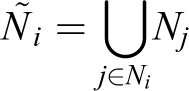
The integrals over $\partial W_{i}^{R} \cap \partial C_{i}^{g s}$ and $\partial W_{i}^{R} \cap \partial H_{i j}$ require knowledge of the AWGV neighbors N_i in order to compute $W_{i}^{R}$ and $H_{i j}$ . Similarly, the integral over $\partial W_{j}^{R} \cap \partial H_{j i}$ requires knowledge of the whole cell $W_{j}^{R}$ of agent j and as such requires information from the AWGV neighbors N_j of agent j. Thus, agent i requires information from all agents in its control neighbors set

${\tilde{N}}_{i} = \underset{j \in N_{i}}{\cup} N_{j}$

which correspond to the AWGV neighbors of all AWGV neighbors of agent i. Given the fact that ${\tilde{N}}_{i} \subseteq I_{n}$ , the resulting control law is distributed, since each agent computes its own control input based on local information.

Constraining agents inside the region

When using control law (10), there is no guarantee that the positioning uncertainty regions of all agents remain completely inside Ω, that is, it is possible that $C_{i}^{u} \cap Ω \neq C_{i}^{u}$ for some agent i. Consequently, the control law may lead some agent i outside the region Ω, given that it may reside anywhere within its positioning uncertainty region $C_{i}^{u}$ .

In order to prevent this from happening, instead of using Ω, a subset $Ω_{i}^{s} \subseteq Ω$ is used instead, which in the general case differs among agents because their uncertainty radii are allowed to be different. This subset of Ω is computed as the Minkowski difference of Ω with the disk $C (r_{i}) = {q \in Ω : ∥ q ∥ \leq r_{i}}$

$Ω_{i}^{s} = {q \in Ω | q + C (r_{i}) \subseteq Ω}, i \in I_{n}$

Using the subset $Ω_{i}^{s}$ , instead of constraining the whole positioning uncertainty regions inside Ω, we need only constrain their centers q_i inside the respective regions $Ω_{i}^{s}$ . This can be achieved by projecting the velocity control input u_i of each agent on $\partial Ω_{i}^{s}$ , resulting in movement along the region’s boundary. This control extension is only required if $q_{i} \in \partial Ω_{i}^{s}$ and the control input u_i leads agent i towards the outside of $Ω_{i}^{s}$ . As a result, the control law extension that guarantees agents remain inside the region is

${\tilde{u}}_{i} = {\begin{array}{l} {proj}_{\partial Ω_{i}^{s}} u_{i} & if q_{i} \in \partial Ω_{i}^{s} \land q_{i} + ϵ u_{i} \notin Ω_{i}^{s} \\ u_{i} & otherwise \end{array}$
14

where ϵ is an infinitesimally small positive constant.

This control enhancement does not affect the monotonic increase of $H$ . This is due to the fact that the inner product of a vector with its projection is always non-negative, thus ${u_{i}}^{T} {\tilde{u}}_{i} \geq 0 \Rightarrow K_{i} {\frac{\partial H}{\partial q_{i}}}^{T} {\tilde{u}}_{i} \geq 0$ . Consequently $\frac{\partial H}{\partial q_{i}} {\tilde{u}}_{i} \geq 0$ which results in monotonic increase of $H$ as shown in the proof of theorem 1.

Inter-agent collision avoidance

Although the derived control scheme guarantees monotonic increase of the coverage objective function $H$ , it cannot guarantee collision avoidance between the agents, since it can result in the overlapping of two or more positioning uncertainty regions. In such a case, it is possible that the agents collide, since their actual positions may reside anywhere within their respective positioning uncertainty regions. In order to avoid overlapping of positioning uncertainty regions, an extension to the control law is devised. Agent i is stopped when the reported distance $∥ q_{i} - q_{j} ∥$ between itself and some other agent j becomes less than or equal to a critical distance $d_{i j}^{c} = r_{i} + r_{j} + ϵ$ , and if the control input leads agent i towards agent j, that is, if ${u_{i}}^{T} (q_{j} - q_{i}) \geq 0$ . ϵ is an infinitesimally small positive constant used so that the control law extension comes into effect before a possible collision. Consequently, each agent i implements

${\tilde{u}}_{i} = {\begin{array}{l} \begin{array}{l} 0, \end{array} & \begin{array}{l} if \exists j \in N_{i} : ∥ q_{i} - q_{j} ∥ \leq d_{i j}^{c} \land \\ {u_{i}}^{T} (q_{j} - q_{i}) \geq 0 \end{array} \\ u_{i}, & otherwise \end{array}$

This procedure is also presented in Algorithm 1.

Algorithm 1:
Collision avoidance – control input ${\tilde{u}}_{i}$ of agent i

It should be noted that this control enhancement does not affect the monotonic increase of $H$ since it either has the same value as the initial control law u_i or zero which results in $H$ being unaffected by this particular agent.

Simplified control law

Due to the complex integrals over $H_{i j}$ and $H_{j i}$ of the complete control law (10), the large amount of information required in order to implement it, as described in remark 4, a simplified control law, using only the first of the three terms of equation (10) is proposed.

Conjecture 1

The control law

$u_{i} = K_{i} \int_{\partial W_{i}^{R} \cap \partial C_{i}^{g s}} n_{i} ϕ d q$
15

is computationally efficient and leads to performance comparable with that of equation (10). However it does not guaranteed the fast convergence rate of the complete control law (10).

Remark 5

The two control law enhancements described in sections “Constraining agents inside the region” and “Inter-agent collision avoidance” are needed both for the complete (equation (10)) and simplified (equation (15)) control laws.

Computational complexity

We will first examine the computational complexity of constructing a single AWGV cell. From equation (3) we get that $W_{i}^{g}$ is the result of $N_{i} + 1$ intersections, where N_i are the AWGV neighbors of agent i. Thus the computational complexity of a single AWGV cell is linear with the number of AWGV neighbors or more formally $O (N_{i})$ .

In order to compute the complete control law (10) each agent i needs to compute its own AWGV cell as well as the cells of its control neighbors ${\tilde{N}}_{i}$ . Thus the total number of intersections required is $(N_{i} + 1) + \sum_{j \in N_{i}} (N_{j} + 1)$ which results in the worst case complexity of this process being $O ({N_{i}}^{2})$ . The complete control law also requires the computation of integrals over the agent’s own cell as well as the cells of all of its control neighbors ${\tilde{N}}_{i}$ . This results in linear complexity $O ({\tilde{N}}_{i})$ , thus the total complexity of the optimal control law is dominated by the quadratic complexity of the creation of the AWGV cells and is $O ({N_{i}}^{2})$ . It should be noted that this is only an upper bound and in practice the computational complexity will be lower than $O ({N_{i}}^{2})$ .

The simplified control law (15) improves on this quadratic complexity by only requiring information from the agent’s AWGV neighbors N_i. Thus, both the cell and integral computations require $O (N_{i})$ time, a significant improvement over the complete control law.

A Monte–Carlo numerical study of the computational cost of both control laws was conducted on an Intel i7-6500U CPU operating at 2.5 GHz. A set of random agent configurations were generated with the number of agents ranging from 3 to 40 and both control laws were computed for all of the agents of each random configuration, resulting in 100,633 measurements. A box plot of the results can be seen in Figure 5, depicting the time needed for the computation of the control input for a single agent with respect to the number of its AWGV neighbors N_i, in blue and red for the complete and simplified control laws, respectively. The circles indicate the median, the bottom and top edges of the filled rectangles the 25th and 75th percentiles, respectively, and the lower and upper whiskers represent measurements that are within 1.5 times the interquartile range (the distance between the 25th and 75th percentiles) from the 25th and 75th percentiles, respectively. It is observed that the simplified control law does indeed approach linear complexity, while the complete control law’s complexity is lower than quadratic in practice, as was expected. The significantly greater variance of the measurements of the complete control law compared to the simplified one is due to the fact that the length of the hyperbolic arcs $\partial W_{i}^{R} \cap \partial H_{i j}$ and $\partial W_{j}^{R} \cap \partial H_{j i}$ varies more than the length of the circular arcs $\partial W_{i}^{R} \cap \partial C_{i}^{g s}$ . It is also observed that the computational time required for the complete control law is significantly longer than that required for the simplified control law.

Figure 5.
Control law computation time in ms versus the number of AWGV neighbors N_i for the complete (blue) and simplified (red) control laws. AWGV: Additively Weighted Guaranteed Voronoi.

Simulation studies

Simulations have been conducted in order to evaluate the efficiency of the complete control law (10) and compare it with the simplified control law (15). The a priori importance of points inside the region was $ϕ (q) = 1, \forall q \in Ω$ . In this case, the maximum possible value for $H$ is

$H^{max} = \sum_{i \in I_{n}} A (C_{i}^{g s})$

where $A (\cdot)$ is the area function, given that n guaranteed sensing disks can be packed inside Ω. In all simulations, the control law extensions as described in sections “Constraining agents inside the region” and “Inter-agent collision avoidance” are used.

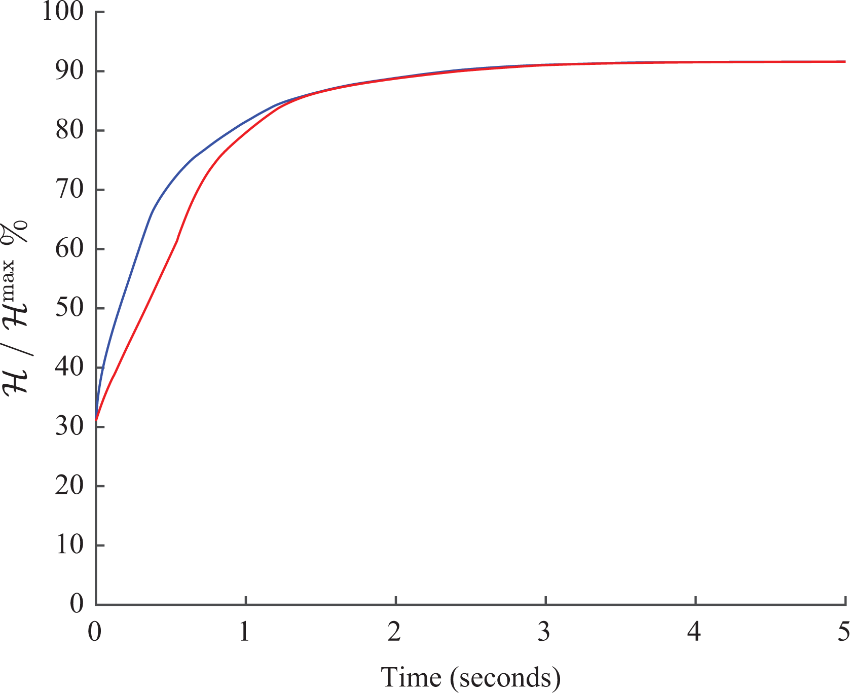
Figures 6, 9, and 12 show the initial and final states of the network for both control laws, with the uncertainty disks shown as filled black circles, the guaranteed sensing disks in dashed blue and the AWGV cells in solid red. The trajectories of the agents are shown in Figures 7, 10, and 13 for both the complete and simplified control laws, with the initial (final) positions represented by circles (squares). Figures 8, 11, and 14 show the evolution of the coverage objective $H$ with time as a percentage of its maximum value, again in blue for the complete and red for the simplified control law.

Figure 6.
Case study I: initial (a) and final configuration for the complete (b) and simplified (c) control laws.

Figure 7.
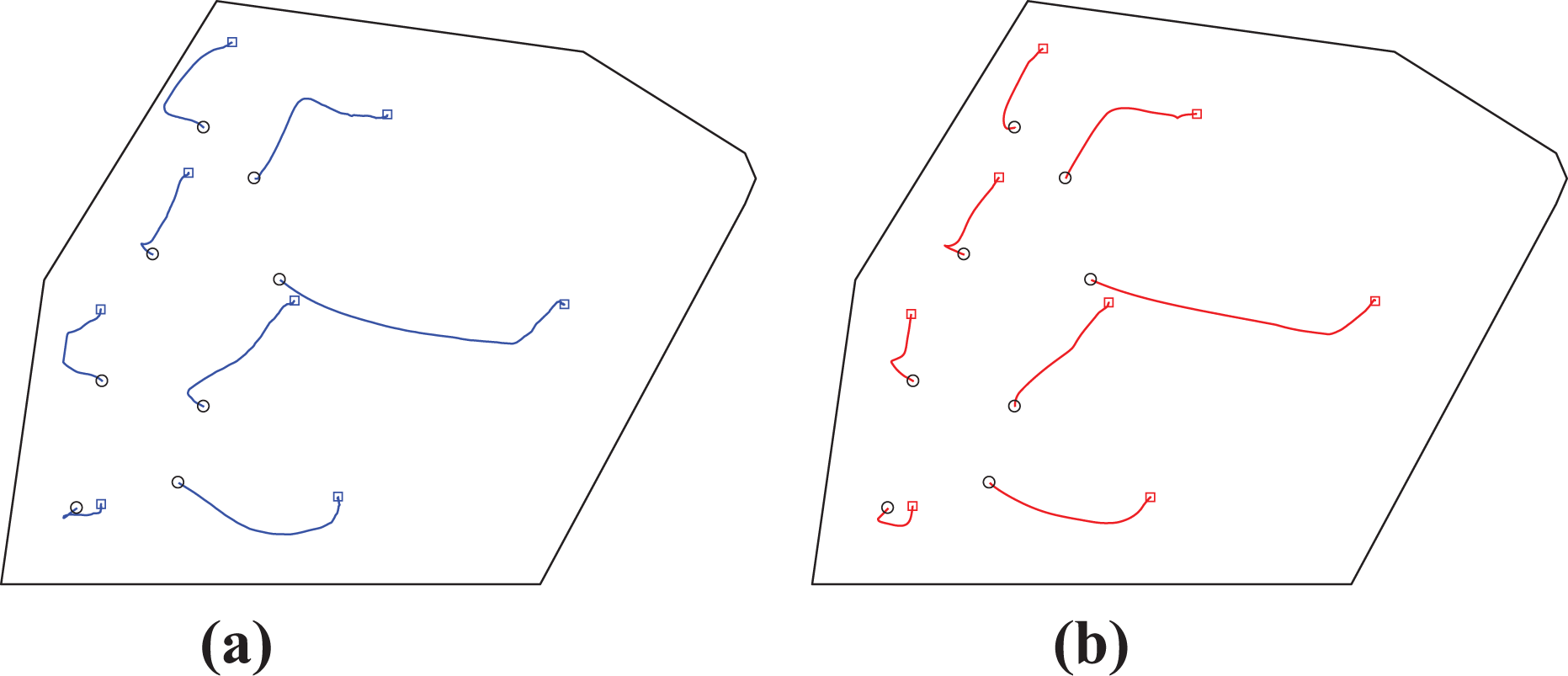
Case study I: agents’ trajectories for the complete (a) and simplified (b) control laws.

Figure 8.
Case study I: evolution of the coverage objective $H / H^{max}$ through time for the complete (blue) and simplified (red) control laws.

Figure 9.
Case study II: initial (a) and final configuration for the complete (b) and simplified (c) control laws when using the virtual sensing radii, resulting in a common guaranteed sensing radius.

Figure 10.
Case study II: agents’ trajectories for the complete (a) and simplified (b) control laws.

Figure 11.
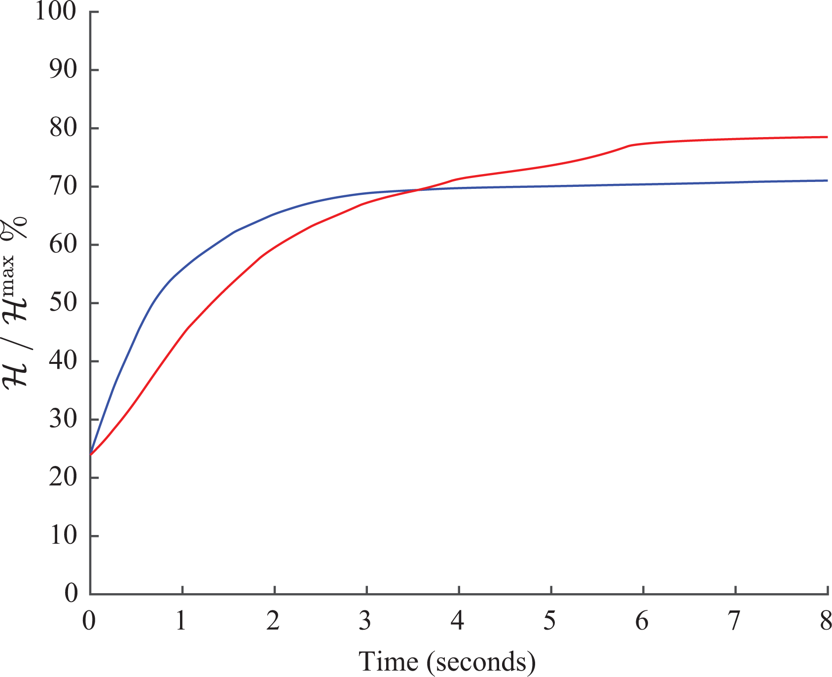
Case study II: evolution of the coverage objective $H / H^{max}$ through time for the complete (blue) and simplified (red) control laws.

Figure 12.
Case study III: initial (a) and final configuration for the complete (b) and simplified (c) control laws.

Figure 13.
Case study III: agents’ trajectories for the complete (a) and simplified (b) control laws.

Figure 14.
Case study III: evolution of the coverage objective $H$ through time for the complete (blue) and simplified (red) control laws.

Case study I

In this case study, an indicative network of eight agents is simulated. Both the uncertainty radii r_i and sensing radii R_i differ between agents. Figure 6 shows the initial and final states of the network for both control laws, Figure 7 shows the agent trajectories, and Figure 8 shows the evolution of the coverage objective $H$ with time as a percentage of its maximum value. It is observed that for both control laws the agents converge to almost identical final configurations, with a mean distance between final agent positions of just 0.40% of the region’s diameter. The coverage objective $H$ increased monotonically in both cases, although this is not guaranteed to happen when using the simplified control law. $H / H^{max}$ has reached a final value of 91.60% for both control laws.

In order to better show the effect of positioning uncertainty in the performance of the agent team, this case study was repeated several times with the same initial conditions for various values of the agents’ positioning uncertainty. Table 1 shows the final value of the coverage objective $H$ for both the complete and simplified control laws where 100% corresponds to the positioning uncertainty in the simulation shown in Figures 6 to 8. It is observed that as positioning uncertainty increases, the final value of the coverage objective decreases, since the area of both the GSRs $C_{i}^{g s}$ and the AWGV cells $W_{i}^{g}$ decreases. It is also observed that the simplified control law achieves the same better performance than the complete one, although not more than 0.2% in these particular simulations. This behavior is further discussed in section “Case study II”.

Table 1.
Dependence of the agents’ performance on their positioning uncertainty.

Uncertainty (%) 0% 25% 50% 75% 100%

Complete 4.5165 4.1024 3.6843 3.3185 2.9742

Simplified 4.5168 4.1104 3.6885 3.3188 2.9742

Case study II

This simulation study is used to present a case where the simplified control law provides better coverage performance than the complete control law. The agents have the same initial configuration as in case study I and the same heterogeneous positioning uncertainty. Their sensing radii are selected so that they have a common guaranteed sensing radius R^g, thus the sensing radius of each agent is ${\tilde{R}}_{i} = R^{g} + r_{i}, \forall i \in I_{n}$ . In this case the AWGV partitioning converges to the GV partitioning and the assigned cells are based solely on the agents’ positioning uncertainty regions. The common sensing radius R^g was selected as the mean of the sensing radii used in case study I.

Figure 9 shows the initial and final states of the network for both control laws, Figure 10 shows the agent trajectories, and Figure 11 shows the evolution of the coverage objective $H$ with time as a percentage of its maximum value. It can be observed that the agent final configuration differs significantly between the complete and simplified control laws, with the mean distance between final agent positions being 11.97% of the region’s diameter. Additionally, one of the agents in the final configuration of the complete control law has been stopped by the control enhancement described in section “Constraining agents inside the region” before crossing the boundary at the top of the region of interest.

However, the most important observation made from this case study is the fact that the simplified control law achieved a higher final value of 78.50% for the coverage objective $H / H^{max}$ , versus a value of 71.03% for the complete control law. It should be stressed that this is due to the nature of gradient-ascent methods leading to local optima. The complete control law leads the agents toward the gradient of $H$ . Consequently the agents move toward the direction that will result in the greatest rate of increase of $H$ . Indeed, it is observed that the complete control law reaches its final configuration sooner than the simplified law. There is no guarantee however that the agents will converge to a global optimum of $H$ , as is the case with all gradient-ascent methods. It is possible that the gradient-ascent control input (equation (10)) leads the agents to a low-value local optimum of $H$ , while a method that does not follow the gradient, such as the simplified control law (15), avoids this particular local optimum and converges to a local optimum with a higher value. Convergence to local optima is a characteristic of such gradient-based distributed control schemes and this case study highlights how different control schemes may converge to different optima of the same optimization function.

Case study III

This case study serves to highlight the need for taking heterogeneous sensing into account when designing the control law. To that extent case study I was repeated with the control law being computed as if the sensing radius of all agents was equal to the smallest sensing radius among agents in case study I. The computation of the value of the coverage objective $H$ however is made with the actual sensing radii which are the same as those in case study I. Figure 12 shows the initial and final states of the network for both control laws and Figure 13 shows the agent trajectories. It is observed that for both control laws the agents converge to almost identical final configurations, with a mean distance between final agent positions of just 0.27% of the region’s diameter. Figure 14 shows the evolution of the coverage objective $H$ with time in solid line for case study III and dashed line for case study I. Blue is used for the complete and red for the simplified control law. Both simulations of case study I converge to a value of 2.97, whereas those of Case Study III converge to final values of 1.62 and 1.63 which corresponds to a decrease in performance of 45%. It is thus shown that taking into account the agents’ heterogeneous sensing performance can lead to significantly improved sensing performance.

Experimental studies

Two experiments were conducted for the evaluation of the simplified control law (15) in the case of homogeneous agents, both in terms of positioning uncertainty and sensing performance. All agents have common positioning uncertainty r and sensing radii R, thus the AWGV partitioning converges to the GV partitioning. The experiments consist of three differential drive robots, an ultra-wideband (UWB) positioning tracking system, and a computer acting as a base station, communicating via a WiFi router.

The utilized robots were the differential drive Arduino UNO DS Robots.³² Although these robots have four powered wheels, they have no steering; thus they are controlled in a manner similar to differential drive robots. These robots lack any kind of positioning system or motor encoders thus an external pose tracking system has to be used. Due to the robots’ lack of omnidirectional sensors, circular sensing patters with a common radius $R = 1 m$ were assumed for the sake of the control law implementation. The robots have a high-level command set that allows them to move forward and backward in a straight line, rotate in place and set the velocity of their motors. Throughout the experiment, their speed was set to the lowest setting of approximately 0.16 m/s. The robots can be inscribed inside a circle with radius $R^{d} = 0.299 m$ .

The Pozyx UWB positioning system³³ was used to measure the robots’ pose. The Pozyx system consists of four stationary anchors and three tags, 1 affixed to each robot. Each tag communicates with the anchors and measures its relative position using time of arrival measurements and multilateration. Apart from the UWB system, the tags are also equipped with an inertial measurement unit and are thus able to measure their orientation in space in addition to their position. Since it is not possible for more than one tag to communicate with the anchors, a fourth tag located at the base station computer was used. This tag acts as a master and synchronizes other tags’ communication with the anchors in a time-division multiple-access manner. The positioning error of our setup was measured in 38 locations, and its maximum measured value of 0.24 m was used as the robots’ common positioning uncertainty radius r.

The experimental setup was as follows. The master tag synchronizes the tags located on the robots and receives their pose measurements. These measurements are sent to the computer which broadcasts them through WiFi. An ODROID-XU4³⁴ computer is affixed on each robot whose purpose is receiving the pose measurements and computing the control input for the robot. Each ODROID-XU4 implements the following loop. The robot’s control input u_i is computed according to equation (15) using the current Pozyx measurements. If u_i is greater than some arbitrary threshold, the robot rotates to match the direction of u_i and moves a small distance in this direction using the high-level command set. Otherwise it remains immobile. The process is then repeated with the new measurements received from the base station computer through WiFi. Each iteration lasts at least 600 ms and varies according to the measure of the angle the robot needs to rotate. It should be noted that the robots were allowed to move both forward and in reverse in order to minimize the magnitude of their rotation.

In all figures regarding the experiments, the region shown is $Ω^{s} \subseteq Ω$ that is, the region inside which the centers of the positioning uncertainty disks are constrained, as described in section “Constraining agents inside the region”. This region is common among all robots since they were assumed to have the same measure of positioning uncertainty. The experiments are compared with simulations with the same initial conditions, that is, robot positions, measure of positioning uncertainty and sensing radii. The region Ω^s was a 3.6 × 4.8 m² rectangle. The robots’ initial and final positions for both the experiments and the respective simulations can be seen in Figures 15 and 19, with the uncertainty disks shown as filled black circles, the guaranteed sensing disks in dashed blue and the GV cells in solid red. The evolution of the coverage objective $H / H^{max}$ can be seen in Figures 18 and 22, in solid blue for the experiment and in dashed red for the simulation.

Figure 15.
Experiment I: initial configuration (a), experiment final configuration (b) and simulation final configuration (c).

Experiment I

The robots’ initial and final positions for both the experiment and the respective simulation can be seen in Figure 15 while photographs of the robots’ initial and final configurations during the experiment can be seen on Figure 16. It is observed from the final robot configurations of both the experiment and the simulation, that all three guaranteed sensing disks are contained completely within their respective GV cells, indicating that the network has reached a globally optimal configuration. Figure 17 presents a comparison between the robot trajectories filtered by a moving average filter with a window of 49 samples and the simulated trajectories where it can be observed that they are not significantly different. Initial and final positions marked with circles and squares respectively. When compared between the experiment and the simulation, the final positions of the agents have a mean distance of 1.34% the diameter of Ω^s. The difference in final configurations is small, considering that for the current number of agents and initial conditions there exist multiple equivalent feasible globally optimal configurations and the differences between the theoretical and implemented control law. However this is not the case in all experiments as will be seen in the next section. 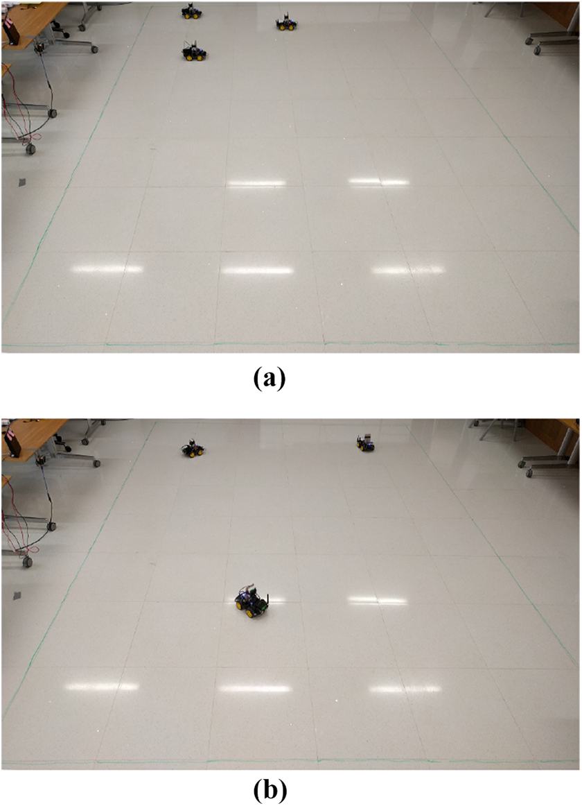The evolution of the coverage objective $H / H^{max}$ can be seen in Figure 18. Although the increase of the coverage objective was not monotonic as a result of the implemented control law, it increased from 62.49% to 99.95% which is the final value attained in the simulation. The spikes in the experimental values are due to measurement noise while more gradual decreases of $H / H^{max}$ are a result of the implementation details such as the robot dynamics and their finite maximum translational and rotational velocities.

Figure 16.
Experiment I: images from the initial (a) and final (b) robot positions during the experiment.

Figure 17.
Experiment I: comparison between the experimental (blue) and simulated (red) robot trajectories.

Figure 18.
Experiment I: evolution of the coverage objective $H / H^{max}$ through time for the experiment (solid blue) and corresponding simulation (dashed red).

Experiment II

For this experiment, the radius R^d of the robots circumcircle was added to their positioning uncertainty radius in order to ensure that each robot is completely contained within its respective positioning uncertainty region $C_{i}^{u}$ . This way, due to the control law extension described in section “Constraining agents inside the region”, it is ensured that the whole robots and not just the positioning uncertainty regions of their centers remain inside the region of interest. Moreover, due to the control law extension described in section “Inter-agent collision avoidance” between the agents can be guaranteed. It should be noted that the guaranteed sensing disks were calculated by taking into account the initial positioning uncertainty and not the one augmented by the robots’ dimensions. The robots’ initial and final positions for both the experiment and the respective simulation can be seen in Figure 19 while photographs of the robots’ initial and final configurations during the experiment can be seen in Figure 20. It is observed from the final robot configurations of both the experiment and the simulation that all three guaranteed sensing disks are contained almost completely within their respective GV cells. Figure 21 presents a comparison between the robot trajectories filtered by a moving average filter with a window of 49 samples and the simulated trajectories. Initial and final positions marked with circles and squares, respectively. When compared between the experiment and the simulation, the final positions of the agents have a mean distance of 24.65% the diameter of Ω^s. Due to the agents’ increased measure of positioning uncertainty compared to the previous case, the resulting GV cells are smaller, which in turn means that the number of local maxima of the objective function $H$ is smaller than in the first experiment. Although it is more probable that in this case, the experiment and simulation will converge to the same configuration, this is not guaranteed to happen. The evolution of the coverage objective $H / H^{max}$ can be seen in Figure 22. Although the increase of the coverage objective was not monotonic as a result of the implemented control law, it increased from 30.15% to 93.40%, while the simulation attained a final value of 99.95%.

Figure 19.
Experiment II: initial configuration (a), experiment final configuration (b) and simulation final configuration (c).

Figure 20.
Experiment II: images from the initial (a) and final (b) robot positions during the experiment.

Figure 21.
Experiment II: comparison between the experimental (blue) and simulated (red) robot trajectories.

Figure 22.
Experiment II: evolution of the coverage objective $H / H^{max}$ through time for the experiment (solid blue) and corresponding simulation (dashed red).

Conclusion

The problem of area coverage of a planar region by a heterogeneous team of mobile agents under imprecise localization is examined in this article. A gradient-based distributed control scheme was designed based on an AWGV partition of the region. The control scheme is extended to ensure the safe operation of the mobile agents and a simplified but computationally efficient control law is also proposed. The two control laws are compared in simulation studies and experiments were conducted to evaluate the efficiency of the simplified control law in a realistic scenario.

Uncertainty (%)	0%	25%	50%	75%	100%
Complete	4.5165	4.1024	3.6843	3.3185	2.9742
Simplified	4.5168	4.1104	3.6885	3.3188	2.9742

Footnotes

Appendix 1 Declaration of conflicting interests

The author(s) declared the following potential conflicts of interest with respect to the research, authorship, and/or publication of this article: This work was partially completed while the authors were with the University of Patras, Greece.

Funding

The author(s) disclosed receipt of following financial support for the research, authorship, and/or publication of this article: This work has received partial funding from the European Union’s Horizon 2020 Research and Innovation Programme under the Grant Agreement No. 644128, AEROWORKS.

ORCID iD

Sotiris Papatheodorou

References

Cortés

Egerstedt

. Coordinated control of multi-robot systems: a survey. SICE J Control Meas Syst Integrat 2017; 10(6): 495–503.

Mahboubi

Aghdam

. Distributed deployment algorithms for coverage improvement in a network of wireless mobile sensors: relocation by virtual force. IEEE Trans Control Netw Syst 2016; 61(99): 1.

Eeden

CFV

Lee

Katsuno

. Minimised moving distance algorithm for geometric deployment of robot swarms. In: Proceeding 55th annual conference of the society of instrument and control engineers of Japan (SICE), Tsukuba, Japan, 20–23 September 2016, pp. 1195–1200. New York, NY: IEEE.

Abbasi

Mesbahi

Velni

. A new Voronoi-based blanket coverage control method for moving sensor networks. IEEE Trans Control Syst Technol 2017; 99: 1–9.

Palacios-Gasós

Talebpour

Montijano

. Optimal path planning and coverage control for multi-robot persistent coverage in environments with obstacles. In: IEEE international conference on Robotics and automation (ICRA), Singapore, 29 May – 3 June 2017, pp. 1321–1327. New York, NY: IEEE.

Bentz

Hoang

Bayasgalan

. Complete 3-D dynamic coverage in energy-constrained multi-UAV sensor networks. Auto Robot 2018; 42(4): 825–851.

Tzes

Papatheodorou

Tzes

. Visual area coverage by heterogeneous aerial agents under imprecise localization. IEEE Control Syst Lett 2018; 2(4): 623–628.

Alitappeh

Jeddisaravi

Guimarães

. Multi-objective multi-robot deployment in a dynamic environment. Soft Comput 2017; 21: 6481–6497.

Stergiopoulos

Thanou

Tzes

. Distributed collaborative coverage-control schemes for non-convex domains. IEEE Trans Autom Contr 2015; 60(9): 2422–2427.

10.

Stergiopoulos

Tzes

. Cooperative positioning/orientation control of mobile heterogeneous anisotropic sensor networks for area coverage. In: Proceeding IEEE international conference on robotics & automation, Hong Kong, China, 31 May–5 June 2014, pp. 1106–1111. New York, NY: IEEE.

11.

Farzadpour

Zhang

Chen

. On performance measurement for a heterogeneous planar field sensor network. In: IEEE international conference on advanced intelligent mechatronics (AIM), Munich, Germany, 3–7 July 2017, pp. 166–171. New York, NY: IEEE.

12.

Kwok

Martinez

. A distributed deterministic annealing algorithm for limited-range sensor coverage. IEEE Trans Control Syst Technol 2011; 19(4): 792–804.

13.

Ramaswamy

Marden

. A sensor coverage game with improved efficiency guarantees. In: Proceeding American control conference (ACC), Boston, MA, USA, 6–8 July 2016, pp. 6399–6404. New York, NY: IEEE.

14.

Cortés

Martinez

Bullo

. Spatially-distributed coverage optimization and control with limited-range interactions. ESAIM: Control Optim Calc Variat 2005; 11(4): 691–719.

15.

Mohseni

Doustmohammadi

Menhaj

. Distributed receding horizon coverage control for multiple mobile robots. IEEE Syst J 2016; 10(1): 198–207.

16.

Mavrommati

Tzorakoleftherakis

Abraham

. Real-time area coverage and target localization using receding-horizon ergodic exploration. IEEE Trans Robot 2018; 34(1): 62–80.

17.

Nguyen

Rodrigues

Maniu

. Discretized optimal control approach for dynamic multi-agent decentralized coverage. In: Proceeding IEEE international symposium intelligent control (ISIC), Buenos Aires, Argentina, 19–22 September 2016, pp. 1–6. New York, NY: IEEE.

18.

Nowzari

Cortés

. Self-triggered coordination of robotic networks for optimal deployment. Automatica 2012; 48(6): 1077–1087.

19.

Habibi

Mahboubi

Aghdam

. Distributed coverage control of mobile sensor networks subject to measurement error. IEEE Trans Automat Contr 2016; 61(11): 3330–3343.

20.

Hage

El Najjar

Pomorski

. Fault tolerant collaborative localization for multi-robot system. In: Proceeding 24th Mediterranean conference on control and automation (MED), Athens, Greece, 21–24 June 2016. pp. 907–913. New York, NY: IEEE.

21.

Davis

Karamouzas

Guy

. C-opt: coverage-aware trajectory optimization under uncertainty. IEEE Robot Autom Lett 2016; 1(2): 1020–1027.

22.

Pierson

Rus

. Distributed target tracking in cluttered environments with guaranteed collision avoidance. In: International symposium on multi-robot and multi-agent systems (MRS), Los Angeles, CA, USA, 4–5 December 2017, pp. 83–89. New York, NY: IEEE.

23.

Zhou

Wang

Bandyopadhyay

. Fast, online collision avoidance for dynamic vehicles using buffered voronoi cells. IEEE Robot Autom Lett 2017; 2(2): 1047–1054.

24.

Papatheodorou

Stergiopoulos

Tzes

. Distributed area coverage control with imprecise robot localization. In: Proceeding 24th Mediterranean conference on control and automation (MED), Athens, Greece, 21–24 June 2016, pp. 214–219. New York, NY: IEEE.

25.

Papatheodorou

Tzes

Giannousakis

. Experimental studies on distributed control for area coverage using mobile robots. In: Proceeding 25th Mediterranean conference on control and automation (MED) , Valletta, Malta, 3–6 July 2017, pp. 690–695. New York, NY: IEEE.

26.

Evans

Sember

. Guaranteed Voronoi diagrams of uncertain sites. In: 20th Canadian conference on computational geometry (CCCG), Montreal, Quebec, 13–15 August 2008, pp. 207–210. CCCG.

27.

Ash

Bolker

. Generalized Dirichlet tessellations. Geomet Dedi 1986; 20(2): 209–243.

28.

Kim

Sugihara

. Voronoi diagram of a circle set from Voronoi diagram of a point set: II. Geometry. Comput Aided Geom Des 2001; 18(6): 563–585.

29.

Jin

Kim

. A sweepline algorithm for Euclidean Voronoi diagram of circles. Comput Aided Des 2006; 38(3): 260–272.

30.

Karavelas

Yvinec

. Dynamic additively weighted Voronoi diagrams in 2D. Algorithms ESA 2002: 586–598.

31.

Flanders

. Differentiation under the integral sign. Am Math Monthly 1973; 80(6): 615–627.

32.

Xiao

. Technology. Arduino UNO DS Robot, http://www.xiao-r.com/Xiaor/?lang=en_us (accessed 15 July 2018).

33.

Pozyx Labs. Pozyx Accurate Positioning,www.pozyx.io/ (accessed 15 July 2018).

34.

Hardkernel. ODROID-XU4,www.hardkernel.com/ (accessed 15 July 2018).