Sage Journals: Discover world-class research

Abstract

The self-reconfigurable modular robot consists of many identical modules. By connecting to/disconnecting from other modules, the whole structure of the robot can transform into arbitrary other configurations. First, the lattice-type self-reconfigurable modular robot is proposed and its disconnected/connected mechanism is analyzed, which can finish self-morphing action. Second, the basic configuration of the module is analyzed with the eigenvector matrix. The motion rules are proposed. Third, the possible motion space is described with the geometric feature of modules which is effective for performing the self-morphing process. Then, the self-morphing motion process is described with the driving function and the adjacency matrix which is useful to solve the computation problem and optimize the motion paths of the robot during the self-reconfigurable morphing process. Final, an experiment of three-module motion and a simulation of multi-module's self-morphing process are shown to prove that the above analyses are effective.

Keywords

Self-morphing Self-reconfigurable Modular Motion space

1. Introduction

Modular self-reconfigurable (MSR) robots consist of a set of standardized electromechanical modules which can dynamically change their geometric structure to complete different task requirements. The MSR robots can be classified as the lattice-type and the chain-type depending on whether their modules use substrate reconfiguration where the modules are placed on a lattice (in either 2D or 3D). Chain-type self-reconfigurable robots have a higher degree of mobility than lattice-type systems do, because the degrees of freedom of chain-type robots are often less constrained than those of lattice-type systems. Lattice-type robots, on the other hand, can easily self-reconfigure and are suitable for forming various static configurations, but they have difficulty in generating motion.

Recently, the research on three-dimensional model has made remarkable progress and many types of robots have been proposed. There are two classes of three-dimensional systems, a class based on lattice systems and a class of linear or string systems. In the former class, the shape of a module is determined by the lattice systems, such as a cubic structure (3-D self-reconfigurable mechanical system) (Murata, S., Yoshida, E., etc, 2001), Fracta 3D (Murata, S., Kurakawa, H., etc, 1998), two hemispheres joined modules (ATRON)(Christensen, D., C., 2006), Telecube(Suh, J. W., Homans, S. B., & Yim, M. H., 2002), the crystal module (Crystalline) (Bulter, Z., & Rus, D., 2003), the “I-Cube” modules (I-Cube) (Unsal, C., & Khosla, P. K., 2000), the rhombic dodecahedron modules (Proteo) (Yim, M., Zhang, Y., etc, 2001), two semi-cylindrical parts (M-TRAN) (Kurokawa, H., Tomita, K., 2008) and M-Cube (Fei, Y.Q., & Zhao, X.F., 2007), (Fei, Y.Q., Zhang, X., & Xia, Z.X., 2009). The latter class of system is a linear or string-type system, such as the cubic modules (Polybot) (Yim, M., Zhang, Y., etc, 2002), the tetrahedral and octahedral modules (Tetrobot) (Hamlin, G. J., & Sanderson, A. C., 1998), CONRO (Castano, A., & Will, P., 2000) and so on.

In this paper, we describe the configuration of a 3-D, like cubic shape, lattice MSR robot called M-Cubes. Its mechanical structure is presented, which can finish self-morphing and self-repairing actions when bad modules appear. The motion rules are proposed. Then, the possible motion space is described with the geometric feature of modules. Thus, each module can calculate its next position according to its neighboring modules and the corresponding three-module motion can be chosen, which is useful for finishing the self-morphing process.

2. Module hardware

2.1. Structure of module

The lattice-type self-reconfigurable modular robot “M-Cubes” (Modular-Cubes) is proposed. Its inner structure and connecting/disconnecting mechanism are different from those of Fracta 3D (S. Murata, H. Kurakawa, etc, 1998). Each module composed of a central cube and six rotary arms distributed on the six sides of the central cube (Fei, Y.Q., Zhang, X., & Xia, Z.X., 2009), as shown in Fig. 1. The rotary arm has a connection shaft and a connection hole. The connection shaft has a lock system, which can lock the connection when the shaft is inserted into other module's hole. Then, two modules can connect to each other firmly. The connecting arm can rotate along its axis.

Fig. 1.

M-Cubes module

Figure 2 shows the inner mechanics of the M-Cubes module. There's a DC motor in the central cube, which is the power supply of the connecting arms. The rotation of the motor is transmitted to the six transmission shafts by a gear system. There's a clutch on each transmission shaft to control whether the connecting arm should rotate or not.

Fig. 2.

Inside mechanics of M-Cubes module

2.2. Disconnected/connected mechanism

The disconnected and connected mechanism is one of the crucial components of a reconnectable module. Due to the unique features of reconfigurable robots, such a mechanism must be power efficient, reliable, compact and flexible to operate.

Each rotary arm (Fig.1, Fig.2.) can connect with/disconnect from other modules. When the robot system needs to finish self-morphing or self-repairing action, the reconnectable side (rotary arm) can finish connecting with or disconnecting from its neighboring side. Especially, when the bad module appears, the reconnectable sides can finish the self-repairing action. If a module is damaged, its neighbors should be able to disconnect it from the system without any constraints from the damaged module. For these purposes, we have designed the disconnected/connected mechanism that allows disconnection to be accomplished at either side of the connection. This is critical for a self-reconfigurable robot to finish the self-morphing action or discard any damaged modules for self-repairing action.

Figure 3 shows this disconnected/connected mechanism of a module. Each rotary arm (reconnectable side) consists of one expansile hole (connection hole) (Fig.4) and one extension peg (connection peg) (Fig.5). The expansile hole mainly consists of two connecting grippers, one cover, one sleeve, one track and one screw rod (Fig.4 c). The hole can open and change its shape when its neighboring module is bad and it needs to disconnect from the bad module and finish the self-repairing action (Fig.4). Generally, the hole keeps closed state (Fig.4 a). When the connection/disconnection appears among good modules, the expansile hole does not open. When a good module wants to disconnect from the bad module, the hole of the good module is open (Fig.4 b) and disconnect from the bad module. Then, this hole returns to its closed state again. When a good module wants to connect to the bad module, the hole of the good module is open and connects to the bad module. Then, this hole returns to its closed state again.

Fig. 3.

The disconnected/connected mechanism of a module

Fig. 4.

The structure of one expansile hole

Fig. 5.

The diagram of one extension peg

The extension peg mainly consists of three beads, a pin, a shell and a piston (Fig.5 b). The hole can accept and lock the incoming peg by meanings of beads. The hole can release a lock by releasing the beads of a good module or open the hole when its neighboring module is bad.

3. Configuration of self-reconfigurable robot

It is important to find an unambiguous, valid and accurate module representation to reduce the M-Cubes system computation and simplify the complexity of the control algorithm in the self-reconfigurable morphing process. Many researchers successfully apply topology theory to solve the module representation. A remarkable effort to formalize this representation was made by Castano and Will (Castano, A., etc, 2002, 2001). They discovered and identified a robot configuration by using graphs and digraphs, and then applied this methodology to the Conro robot. Saidani proposed a distributed algorithm which transforms a quadruped robot into a chain by defining the notion of the graph topodynamics (Saidani, S., 2004).

In the M-Cubes system, a module is represented as a vertex, and a connection between modules as an edge.

3.1. Single module

To express clearly the position of each module, the coordinate systems are set up (Fig. 6). ∑_o is a global coordinate system. ∑_i (i=1, 2,…n) is the local coordinate system whose origin is at the center of each module and whose axes are vertical to rotary sides. A line from the center of the peg to the center of the hole is defined as the peg-hole line (Fig. 7). In order to understand the state of each rotary side, the eigenvector matrix is used to describe each module.

Fig. 6.

The coordinate system

Fig. 7.

The peg-hole line

For the rotary sides which are vertical to the axis X: If the peg-hole line points to the direction of the axis Z, the state is 1, or else it is −1. If the peg-hole line points to the direction of the axis Y, the state is 2, or else it is −2.

For the rotary sides which are vertical to the axis Y: If the peg-hole line points to the direction of the axis Z, the state is 1, or else it is −1. If the peg-hole line points to the direction of the axis X, the state is 2, or else it is −2.

For the rotary sides which are vertical to the axis Z: If the peg-hole line points to the direction of the axis X, the state is 1, or else it is −1. If the peg-hole line points to the direction of the axis Y, the state is 2, or else it is −2.

Each module can be depicted with eigenvector L_i (s₁, s₂, s₃, s₄, s₅, s₆) (s_j denoting eigenvalue, j=1,2,3,4,5,6, s₁ is on +X side, s₂ is on -X side, s₃ is on -Y side, s₄ is on +Y side, s₅ is on +Z side, s₆ is on -Z side,). In order to obtain the state of each rotary side from the topology graph, we give some rules. The solid arrow detaching from this, s_j represents 1 and the virtual one represents −1. The solid arrow pointing to this side, s_j represents 2, and the virtual one represents −2.

3.2 Configuration of the multi-module system

For multi-module system, the following rules are given:

If there is nothing on the rotary side, the value of s_j is 0 and the arrow is not used.

If there is an obstacle on the rotary side, the value of s_j is 4 and the arrow is not used.

If two modules are connected, the values of s_j in the two connecting sides are 3. The two sides are connected with a solid line.

If there is a module on some rotary side but they are not connected. The above rules are used.

Thus, the self-reconfigurable robot with n modules can be described with nx6 eigenvector matrix (Fig. 8).

\begin{aligned} s_{1} s_{2} s_{3} s_{4} s_{5} s_{6} \\ \begin{matrix} L_{1} \\ L_{2} \\ L_{4} \\ L_{5} \\ L_{3} \\ L_{6} \\ L_{8} \\ L_{9} \\ L_{7} \\ L_{10} \\ L_{12} \\ L_{11} \end{matrix} [\begin{matrix} 0 & 3 & 0 & 3 & 3 & 0 \\ 0 & 3 & 3 & 0 & 3 & 0 \\ 3 & 0 & 0 & 3 & 3 & 0 \\ 0 & 3 & 0 & 3 & 3 & 3 \\ 3 & 0 & 3 & 0 & 3 & 0 \\ 0 & 3 & 3 & 0 & 3 & 3 \\ 3 & 0 & 0 & 3 & 3 & 3 \\ 0 & 1 & 0 & - 1 & 0 & 3 \\ 3 & 0 & 3 & 0 & 3 & 3 \\ 0 & - 1 & 1 & 0 & 0 & 3 \\ 2 & 0 & 0 & - 1 & 0 & 3 \\ 1 & 0 & - 1 & 0 & 0 & 3 \end{matrix}] \end{aligned}

(1)

Fig. 8.

The topological structure of 12-module robot system

From (1), the configuration of the self-reconfogurable robot with 12 modules (Fig. 8) can be obtained.

4. Motion rules of the self-reconfigurable robot

According to the geometric feature of the self-reconfigurable robot, there are three kinds of motion: single module motion, two-module motion and three-module motion.

4.1. Single module motion

There are six sides in each module. Each side can rotate 90°, −90° and 180° (Fig. 9). Thus, there are 18 kinds of single module motion.

Fig. 9.

Basic motion of single module

We use rotP(m_i, p_α, θ) to describe the single module motion. Here rotP stands for the single module motion, m_i stands for the i-th module, (i = 1, 2, …, n), p_α stands for the rotary sides (α = 1, 2,…,6), θ stands for the rotary angles (θ= 90°, −90° or 180°).

4.2. Two- module motion

There are two kinds of two-module motion. One is connection or disconnection between two modules. We use conP (m_i, m_j, p_iα, p_jβ) or disconP (m_i, m_j, p_iα, p_jβ) to describe this kind of motion, respectively. Here i, j = 1, 2,…, n; α, β = 1, 2, …, 6, m_i, m_j stand for two neighboring modules, p_iα, p_jβ stand for the rotary sides. The other is the rotary motion between two modules (Fig. 10). We use rotM(m_i, m_j, p_iα, θ) to describe this kind of motion. Here rotM stands for the rotary motion, m_j stands for the basic module (j=1,2,…n and j≠i), θ stands for the rotary angle between two modules.

Fig. 10.

Rotary motion of two modules

4.3. Three- module motion

Three-module motion can really change the positions of the modules. Three modules are named as follows: a base module, a rotary axis module and a motion module. In the XY plane, there are three kinds of three-module motion (Fig. 11). In Fig. 11 a, the rotary axis module rotates 90° or −270°. In Fig. 11 b, the rotary axis module rotates −90° or 270°. In Fig. 11 c, the rotary axis module rotates ±180°.

Fig. 11.

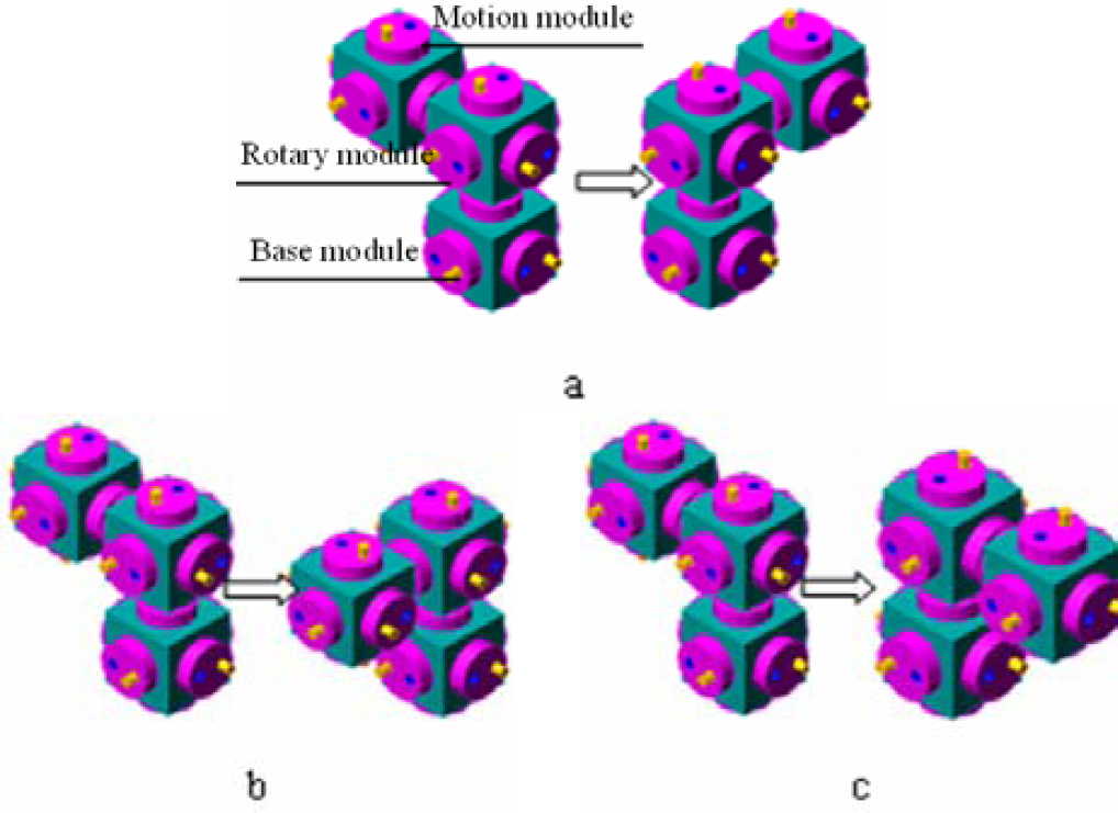
Three-module motion

We can use movM (m_i, m_j, m_k, θ) to describe the three-module motion. Here movM stands for the three-module motion. m_j stands for the base module. m_k stands for the rotary axis module, j,k=1, 2,… n, j ≠k≠i. θ stands for the rotary angle between two modules.

5. Possible motion space

According to the rules of the chessboard and the basic motion of modules, single module of the lattice-type self-reconfigurable robot can change its space position only with its neighboring modules. In order to perform the morphing motion of the lattice-type self-reconfigurable robot, all possible spaces' positions which the module can arrive at must be studied. Then the self-morphing process can be done.

The motion space of the self-reconfigurable robot can be divided into several small cubes which are same as modules. The coordinate system (Fig.12) can be set up. The origin of the coordinate system is on the center of one bottom module. Assuming each module is a 1×1×1 cube, the center coordinate of each module can be marked. All possible motion spaces of modules can be described with these coordinates

Fig. 12.

Motion space of self-reconfigurable robot

Each module can move in the XY plane, YZ plane and XZ plane. We will describe the possible motion spaces of modules in the XY plane, the other two are the same. In Fig.13, the rotary module and the base module are superposed. In the XY plane, there are four possible rotary axes around one module. According to the number and the position of the axes, the possible motion spaces of modules are not the same. Assuming the coordinate of the motion module is (x, y, z).

Fig. 13.

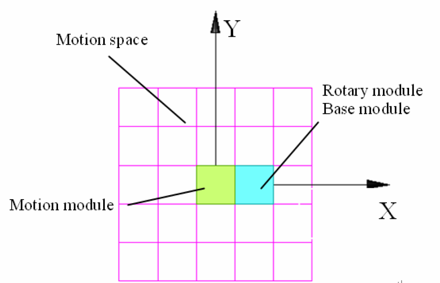
Module's motion space

If there are four rotary axes around the motion module, the module cannot move in the XY plane. Thus, the possible motion space is 0.

If there are three rotary axes around the motion module, the possible motion spaces are (x±1, y±1,z), (x, y±2,z), (x+2,y, z)(Fig.14 a). (x±2, y, z), (x±1, y±1,z), (x, y+2, z)(Fig.14 b). Each has four kinds of motion spaces.

If there are two rotary axes around the motion module, there are three kinds of layout. Thus, the possible motion spaces are:

(x±1, y±1,z), (x±2, y, z) (Fig.15 a); (x+2, y, z), (x, y+2, z), (x±1, y+1, z) and (x+1, y−1,z) (Fig.15 b), (x, y−2, z), (x+2, y, z), (x±1, y−1,z) and (x+1, y+1,z) (Fig.15 c); In Fig.15 a, each module has six kinds of possible motion spaces. In other figures, each module only has five kinds of possible motion spaces.

If there is only one rotary axis around the motion module, there are one kind of layout. Thus, the possible motion spaces are: (x+1, y±1,z), (x+2, y, z). Each module has three kinds of possible motion spaces.

Fig. 14.

The motion space in the XY plane of module that has 3 axes

Fig. 15.

The motion space in the XY plane of module that has 2 axes

Fig. 16.

The motion space in the XY plane of module that has one axis

According to the above analysis, if there are two rotary axes around the motion module, there are the most possible motion spaces. If there are more or less two rotary axes around the motion module, it is not benefit to the movement of the module. With one or two three-module motion, modules can arrive at their next position. In order to perform the morphing process, the possible motion spaces must be obtained. Thus, each module can calculate its next position according to its neighboring modules and the corresponding three-module motion can be chosen.

6. Self-morphing motion process

6.1. Self-morphing Motion Planning Algorithm

The M-Cubes system is a nonlinear system with multi-degree of freedom. As more modules are added to the system, the possible reconfiguration of a group of modules from an initial configuration to a final configuration based on some constraints increases exponentially. This leads to computational complexity in determining an optimal or a near optimal method. So a morphing method based on a driving function and the adjacency matrix is selected to give a near optimal solution. In the initial reconfiguration phase, the driving function is utilized to drive modules to the geometry center of the final configuration based on the local rules. Compared with the method used in (Tomita, K., Murata, S. & Yoshida, E. 1998), (Yoshida, E., Murata, S. & Kurokawa, H. 1998, 2001), our method based on the local rules can reduce the system computation. When a module reaches the vicinity of the final configuration's geometric center, the driving function dies and the adjacency matrix will be used to compute the steps from each module position to the present goal position, and then the minimal steps are selected. By repeatedly adjusting modules coincidence with unoccupied objective position, the final configuration can be completed. The geometric center G_g of the final configuration and the distance S^t_i between the center of module i and G_g at time t can be expressed as follows:

G_{g} (x_{g} y_{g} z_{g}) = \sum_{i = 1}^{M} G_{i}^{f} (x_{g} y_{g} z_{g}) / n

(2)

S_{i}^{t} = | x_{i}^{t} - x_{g} | + | y_{i}^{t} - y_{g} | + | z_{i}^{t} - z_{g}

(3)

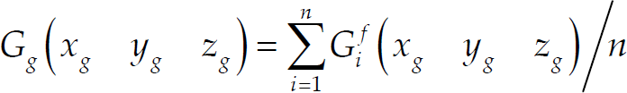
The difference between S^t_i and S^t+1_i could be used as the driving function f_i=S^t_i-S^t+1_i. When module i moves to one direction so that the value of f_i is bigger, this motion direction will be more encouraged. If the value of f_i is negative, this motion direction will be discouraged.

The motion priority in the reconfiguration process is shown in equation (4)

δ_{i} (t) = α \cdot S_{i}^{t} + (β / λ_{i}^{t})

(4)

The motion priority of a module is decided by two factors: S^t_i, Λ^t_i. Λ^t_i is utilized to express the number of the neighborhood module connecting with module i at time t, called the degree of module i at time t. In other words, Λ^t_i indicates the edge number of the node m_i connecting with the other nodes. Obviously, if a module is farther from the center of the final configuration or the number of Λ^t_i for this module is smaller, this module has more motion priority. Different value of coefficient α, β will influence different reconfiguration sequence between modules, and then bring into being different possible motion paths and steps when the system completes the final configuration. As a result of our experiments, the right value of coefficient α, β are decided by the module number of the robot system and the distance between the start location and the goal location.

In the start phase, control of the reconfiguration consists of the following three steps. Each module (1) tests if it is movable and, if so, calculates the value of δ_i(t); (2) compares the value of δ_i(t) with neighboring modules by the local communication. If the value of δ_i(t) is biggest in the neighboring modules, module i calculates all the reachable positions and prepares for moving. If the value of δ_i(t) is equal to that of some neighboring modules but bigger than that of the others, the system randomly selects one of modules having biggest priority value and prepares for moving this module; (3) calculates the value of f_i in all the reachable positions. If all values are negative numbers, this module stops moving. If some values are positive numbers, module i moves to the position producing bigger value of f_i.

There will be at least one module motion at one time based on above rules. Parallelism insures the stabilization and scalability of the system. When module i reaches at most one unit distance from the center of final configuration (S^t_i⩽1), the system changes the control algorithm and starts another control algorithm to complete the final configuration. In order to select minimal steps to reach the desired location, we define the following lattices space set:

S^t_m is the lattice space set that the configuration at time t is occupying.

S^t_p is the unoccupied lattice space set at time t that movable modules in the present configuration can reach in only one reconfiguration process. Obviously, S^t_m∩S^t_p=Ø.

S_f is the lattice space set that the final configuration possesses.

Based on the above three sets, four intersections are defined as follows:

\begin{aligned} S_{n}^{t} = S_{p}^{t} \cap S_{f}, S_{o}^{t} = S_{m}^{t} \cap S_{f}, \\ S_{q}^{t} = S_{m}^{t} \cap \bar{S_{f}}, S_{j}^{t} = S_{m}^{t} \cup S_{p}^{t} = (S_{o}^{t} + S_{q}^{t}) \cup S_{p}^{t} \end{aligned}

Depth first search algorithm can be used to find the topology structure of S^t_j. The adjacency matrix A_t can be expressed as (5):

A^{t} = (a_{i j}^{t} K \times K)

(5)

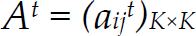
K is the element number of set S^t_j. V_i is the lattice space of set S^t_j. At time t, if a module at the lattice space V_i can reach the lattice space V_j in only one step, a^t_ij is equal to 1.

If it cannot, a^t_ij is 0. If a module at the lattice space V_i cannot reach the lattice space V_j under any circumstances, a^t_ij is ∞. The adjacency matrix A^t is utilized to represent in how many steps a module reach another lattice space of set S^t_j. The system planner only moves non-overlapped modules in set S^t_q to non-overlapped module positions in set S_f until the reconfiguration is complete. If a^t_ij is equal to 1 and V_i∈S^t_q, V_j∈S^t_n, the system planner moves module i to the position V_j. If the above condition does not exist, the system planner computes the square of A^t as follows.

(A^{t})^{2} = (A^{t}) ∙ (A^{t}) = {((a_{i j}^{t})^{2})}_{K \times K}

(6)

Where

(a_{i j}^{t})^{2} = \sum_{i = 1}^{K} a_{i j}^{t} a_{i j}^{t}

(7)

It can be seen by equation (7) that a^t_ila^t_lj is not equal to 0 under condition that only a^t_il and a^t_lj are 1. It means if a^t_ila^t_lj is not equal to 0, the module can start from position V_i, via position V_l, then to position V_j. So the value of (a^t_ij)² denotes how many paths the module can start from position V_i to position V_j in two steps. If modules in set S^t_q cannot reach the position in set S^t_n in one step, the system planner computes (A_t)² and tries to find if there is a path finish the task. If it cannot, the system planner continues to compute (A_t)³ and so on until the module in position V_i moves to the goal position V_j. The final configuration will be competed by repeating the above reconfiguration process.

6.2. Experiment and Simulation

An experiment about the basic motion of a three-module self-reconfigurable robot is shown in Fig.17. Only one module cannot change its own position. There should be at least 3 modules if the position of one module needs to be changed. As shown in Fig. 17 a, the rotary arm of module 1 that connects to module 2 rotates along its own axis so that module 2 rotates with it. Because module 2 has a firm connection to module 3 by one of its arms, module 3 rotates as well. Consequently, the position of module 3 is changed, while the positions of module 2 and module 1 remain the same as before, shown in Fig.17 b. This is the basic morphing motion of M-Cubes modules.

Fig. 17.

Basic morphing motion of a three-module self-reconfigurable robot

Fig. 18.

Simulation of the self-morphing process

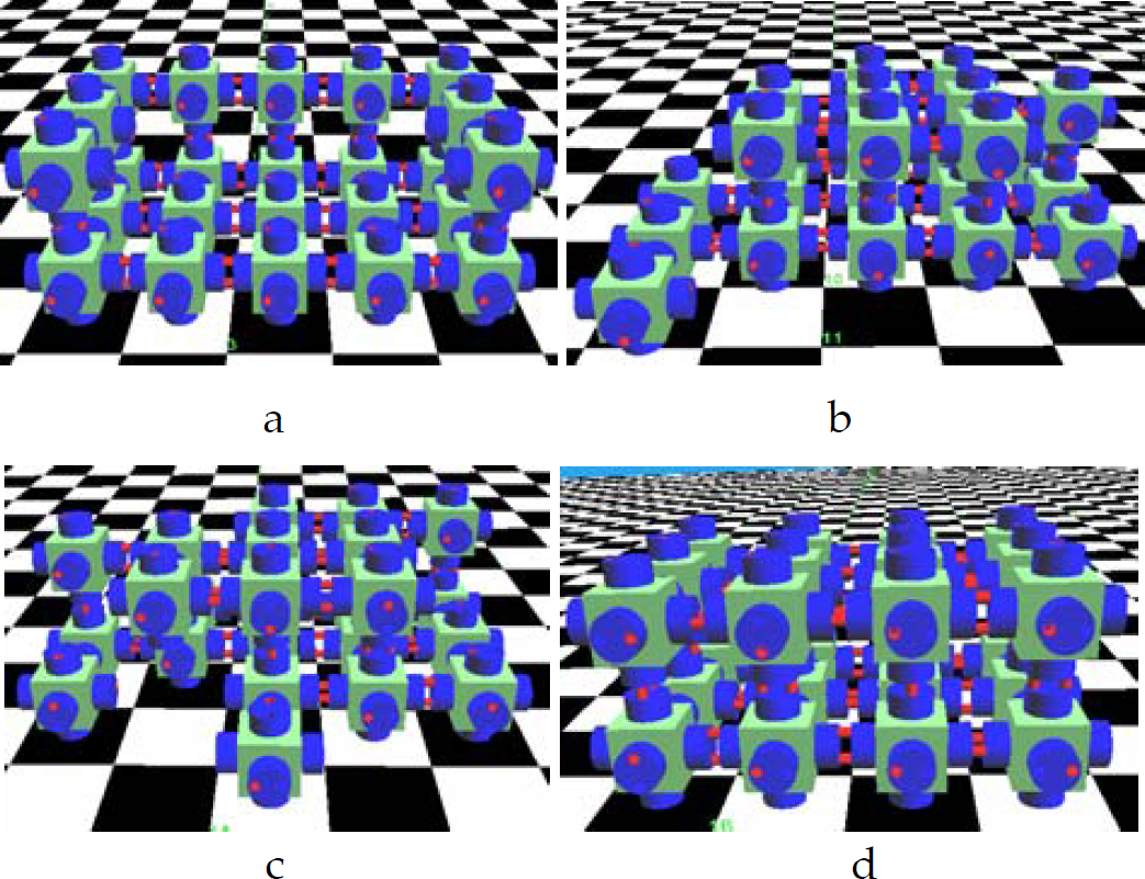
A simulation of the self-morphing process is shown in Fig. 18 under condition that gravity, friction and inertia etc are negligible. The initial configuration is the couch-shaped (Fig.18.a). Fig. 18.b shows snapshots of the first self-morphing phase. Fig. 18.c is a snapshot showing that a module reaches at most one unit distance from the center of final configuration. Fig. 18.d shows the final configuration. The simulation results prove that above self-morphing algorithm is highly efficient.

7. Conclusion

In this paper, we have presented a lattice, self-reconfigurable modular robot. Each module composes of a central cube and six rotary arms. On each rotary arm, there are one expansile hole (connection hole) and one extension peg (connection peg). This structure can make the modular robot system finish self-morphing or self-repairing action when the bad modules appear. The basic configuration of the modules is analyzed with the eigenvector matrix. The model can express information on modules position, connecting relationship and so on. The possible motion rules are proposed. And the possible motion space based on the geometric feature is described which is useful to finish the self-morphing process in the lattice-type self-reconfigurable robot. Then, a new self-morphing motion method based on the driving function and the adjacency matrix is described. The method provides a shortest path from the initial configuration to the final configuration. Finally, an experiment about the basic morphing motion of a three-module self-reconfigurable robot is presented, and a simulation of multi-module self-morphing motion process is shown to prove that the analyses are effective.

Footnotes

8.

This work is supported by NSFC Grant 50305021, 50775145 and State Key Laboratory of Robotics (No.RL0200906).

References

Bulter

& Rus

(2003). Distributed planning and control for modular robots with unit-compressible modules. The International Journal of Robotics Research, Vol. 22, No. 9, pp 699–715.

Castano

Behar

& Will

(2002). The conro modules for reconfigurable robots. IEEE/ASME Transactions on Mechatronics, Vol. 7, No.4, pp 403–409.

Castano

& Will

(2001). Representing and Discovering the Configuration of Conro Robots. Proc. of the 2001 IEEE International Conference on Robotics and Automation, pp.3503–3509, Seoul, Korea.

Castano

& Will

(2000), Mechanical design of a module for reconfigurable robots, Proceeding of IEEE Conference on Intelligent Robots and Systems, pp 2203–2209, Takamatsu, Japan.

Christensen

D. J.

& Stoy

(2006), Selecting a meta-module to shape-change the ATRON self-reconfigurable robot, Proceeding IEEE International Conference Robotics and Automation, pp 2532–2538, Orlando, Florida, USA.

Fei

Y.Q.

& Zhao

X.F.

(2007). Design and dock analysis for the interactive module of a lattice-based self-reconfigurable robot. Robotics and Autonomous Systems, Vol.55, No.2, pp 87–95.

Fei

Y.Q.

Zhang

, & Xia

Z.X.

(2009). Motion Spaces and Self-morphing Algorithm of Self-reconfigurable Modular Robot. Journal of Mechanical Engineering, Vol.45, No.3, pp 197–202.

Hamlin

G. J.

& Sanderson

A. C.

(1998). Tetrobot: A Modular Approach to Reconfigurable Parallel Robotics, Newton, MA: Kluwer Academic, 1998.

Kurokawa

Tomita

Kamimura

Kokaji

Hasuo

Murata

(2008). Distributed Self-Reconfiguration of M-TRAN III Modular Robotic System. The International Journal of Robotics Research, Vol.27, No.(3–4), pp 373–386.

10.

Murata

Yoshida

Kurokawa

Tomita

and Kokaji

(2001). Self-repairing mechanical systems. Autonomous Robots, 10, pp 7–21.

11.

Murata

Kurakawa

Yoshida

Tomita

Kokaji

(1998), A 3-D self-reconfigurable structure, Proceedings of IEEE International Conference on Robotics and Automation, pp 432–439.

12.

Saidani

(2004). Self-Reconfigurable Robots Topodynamic, Proceedings of the 2004 IEEE International Conference on Robotics and Automation, pp 2883–2887, New Orieans.

13.

Suh

J. W.

Homans

S. B.

& Yim

M. H.

(2002). Telecubes: mechanical design of a module for self-reconfigurable robotics, Proceeding of IEEE Int. Conf. on Robotics and Automation (ICRA), pp 4095–4101, Washington D.C., USA.

14.

Tomita

Murata

& Yoshida

(1998). Reconfiguration method for a distributed mechanical system, Proceeding of the 1998 IEEE International Conference on Robotics and Automation, pp 860–865.

15.

Unsal

& Khosla

P. K.

(2000). Mechatronic design of a modular self-reconfigurable robotics system, Proceeding of IEEE Int. Conf. on Intelligent Robots and Systems, pp 1742–1747, Takamatsu, Japan.

16.

Yim

Zhang

Lamping

& Mao

(2001). Distributed control for 3-D metamorphosis. Autonomous Robots, 10, pp 41–56.

17.

Yim

Zhang

Roufas

Duff

& Eldershaw

(2002). Connecting and disconnecting for chain self-reconfiguration with PolyBot. IEEE/ASME Transactions on Mechatronics, 7, pp 442–451.

18.

Yoshida

Murata

& Kurokawa

(1998). A distributed reconfiguration method for 3-D homogeneous structure, Proceeding of the 1998 IEEE International Conference on Intelligent Robots and Systems, pp 852–859.

19.

Yoshida

Murata

& Kamimura

(2001). Reconfiguration planning for a self-assembling modular robot, Proceeding Of the 4^th IEEE International Symposium on Assembly and Task Planning Soft Research Park, pp 276–281, Fukuoka, Japan.

Analysis on Self-Morphing Process of Self-Reconfigurable Modular Robot

Abstract

Keywords

1. Introduction

2. Module hardware

2.1. Structure of module

3.1. Single module

4.1. Single module motion

6.1. Self-morphing Motion Planning Algorithm

Footnotes

8.

References