
Abstract
While navigating in a typical traffic scene, with a drastic drift or sudden jump in its Global Positioning System (GPS) position, the localization based on such an initial position is unable to extract precise overlapping data from the prior map in order to match the current data, thus rendering the localization as unfeasible. In this paper, we first propose a new method to estimate an initial position by matching the infrared reflectivity maps. The maps consist of a highly precise prior map, built with the offline simultaneous localization and mapping (SLAM) technique, and a smooth current map, built with the integral over velocities. Considering the attributes of the maps, we first propose to exploit the stable, rich line segments to match the lidar maps. To evaluate the consistency of the candidate line pairs in both maps, we propose to adopt the local appearance, pairwise geometric attribute and structural likelihood to construct an affinity graph, as well as employ a spectral algorithm to solve the graph efficiently. The initial position is obtained according to the relationship between the vehicle's current position and matched lines. Experiments on the campus with a GPS error of dozens of metres show that our algorithm can provide an accurate initial value with average longitudinal and lateral errors being 1.68m and 1.04m, respectively.
1. Introduction
Rapid progress in mapping and localization with cameras and/or lidar scanners has turned self-driving vehicles into reality over the past several years. An autonomous vehicle needs to understand its surrounding environment. In contrast to directly using a vehicle's sensors to perceive the unknown three-dimensional (3D) environment, such as lane marking [1–3] and dynamic vehicles [4], the localization in a prior map can greatly assist the vehicle to understand the environment, as the information contained in the prior map could be utilized to aid environmental perception.
In order to localize against the prior map, the localization module firstly needs to extract a portion from the prior map, according to the current position provided by a GPS or a GPS-aided inertial navigation system (INS). In most circumstances, the GPS can provide metre-level accuracy, which can ensure that there are enough overlapping areas between the extracted prior data and the current collected data. Based on the assumption, most approaches set an upper bound on the initial position error at a few metres. For example, [5] assumes the drift to be in the order of metres, [6] constrains the error to 3.5m, [7] thinks the error of 3m is the maximum, [8, 9] limit the error within 1.5m, and [10] also limits the search to the range of 1.5m. The assumption is feasible when the GPS signal has no severe drift or jump. After that, based on the overlapping area, the precise localization can be achieved by data registration. In the process of the localization, the GPS plays the role of providing an initial guess. Unfortunately, in some specific traffic scenarios, the GPS signal can be disturbed by the occlusions of vegetation, buildings or multi-path effects due to reflections, which makes the GPS error as large as tens of metres or even more. The assumption of the initial position with metre-level accuracy cannot be satisfied. Thus, there are not enough overlapping areas between the current data and the prior data in the alignment, rendering the localization as unfeasible.
In order to overcome the drift and sudden jump of GPS in the localization, an effective strategy is needed to provide a reliable initial position estimate. Thus, the localization module can be successfully initialized and then proceed using typical data registration approaches. Unfortunately, according to the references published to date, research on this topic has rarely been conducted. We focus on this problem in this paper.
We first propose a new algorithm to estimate the initial position by line segment matching in lidar intensity maps. The SLAM techniques [11–14] are considered as an optimal option to generate the map because of its highly accurate mapping ability. We use the offline SLAM technique [14] to build the prior map. Meanwhile, we build the current smooth map with the integral over velocities from an INS. Considering the special attributes of the lidar intensity map, rather than using the SIFT feature [15], typically used in the computer vision field, we propose to adopt the stable, rich line segments to match the lidar maps. To measure the pairwise consistency, we propose to combine the local appearance, pairwise geometric attribute and structural likelihood to construct the affinity graph for the candidate line pairs, as well as employ a spectral technique [16] to solve the matching problem efficiently. In contrast to reference [17], the addition of the structural information between neighbouring lines can well describe the difference between them, which is a similar measuring process to that in [17]. One main contribution of our method is that it can more accurately distinguish the lines detected in the repeated regions that usually appear in the lidar map, while [17] cannot. The initial position estimate in the prior map is obtained by calculating the relationship between the current vehicle's position and the matched lines. Experiments on campus with GPS errors of dozens of metres show that our algorithm can always provide an accurate initial position estimate with an average longitudinal and lateral error of 1.68m at its maximum, which is satisfied by the need of the initial guess in the localization.
The rest of the paper is organized as follows. In the next section, a survey of related studies is summarized. After that, we present the details about constructing the maps, as well as analyse their attributes. Line segment matching in maps is presented in Section IV. The estimation of the initial position is described in Section V. The experimental results and analysis are shown in Section VI. The last section presents our conclusions.
2. Related Works
Large-scale, long-term outdoor localization in the field of autonomous driving has attracted considerable research interest since the DARPA Urban Challenge of 2007. Early visual localization algorithms focused on designing interest point features to construct a probability distribution over the belief pose and the feature map in the extended Kalman filter (EKF) [18] or FastSLAM [19] framework. To enhance the robustness of the low-level point feature under different illumination conditions, Doersch et al. [20] proposed a method to extract the middle-level image patches with distinctive geometric attributes from a collection of images of London and Paris. This method was shown to be able to pick out image patches, or visual elements, of balconies, windows and street signs, which can easily distinguish the Parisian streets from the London streets. Inspired by [20], Colin et al. [5] presented an unsupervised system to learn about the spatially indexed detectors for distinctive visual elements, in which the localization task is transformed into matching the detectors. In high-level, whole image-based localization, Stewart et al. [21] proposed to exploit a 3D map to localize the monocular camera by minimizing the normalized information distance between the appearance of 3D lidar points reprojected onto overlapping images. Recently, Wolcott et al. [10] localized the vehicle by maximizing the normalized mutual information between the live camera images and the synthetic views within a 3D prior ground map, generated by the survey vehicle equipped with a 3D lidar scanner. However, the image-based localization approach could be easily influenced by abrupt lighting changes.
Given the lidar's insensitivity towards lighting changes and its precise range measurements, the localization with lidar has attracted more and more attention, as well as having been widely applied in recent years. Localization approaches, based on lidar, mainly focus on the point level because of its high accuracy. Hata et al. first proposed the detection of curb points [1] in a 3D lidar point cloud, later extending the approach to extract road markings [2] in reflective intensity data. Those points were fed into the Monte Carlo framework to localize the vehicle. The drawback of the two methods lies in the fact that they cannot adequately constrain the longitudinal error on a long straight road. Baldwin et al. [6] proposed to exploit a dual-lidar system: one oriented horizontally for inferring vehicle linear and rotational velocity, and the other declined to capture a dense view of the environment. Zhu et al. [22] combined the iterative closest points algorithm and terrain inclination knowledge in order to localize. To handle the highly dynamic changes in an industrial environment, a dual-timescale normal distributions transform Monte Carlo localization (NDT-MCL) algorithm is proposed in [23], which simultaneously keeps track of the pose using a prior static map and a short-term current map; the position was decided by matching the current scan to the best timescale map. Markus et al. [3] manually labelled curbs and road markings in a highly accurate lidar intensity map, in which the vehicle's pose was determined by matching the measurement points in the current camera image and the sampled points from the labelled line segments. Jesse et al. used infrared reflectivity from 3D lidar to build an orthographic high-resolution ground map [8] and a probabilistic map [9]; online localization was then performed with the current 3D lidar measurements and a combination of GPS-aided INSs. Recently, reference [24] presented the localization of a vehicle in dense urban areas in which GPS-based methods failed. This study first exploited a visual-based method to process georeferenced landmarks obtained by a learning path and stored landmarks in the geographical information system (GIS), after which the geometric model, GPS data and odometric data were combined in order to localize. This method can obtain reliable positions with few failures, although the drawback lies in the fact that it only works well in areas covered by a GIS.
Existing methods to match lines can be divided into three types: matching individual line segments, matching groups of line segments and matching lines by employing point correspondences.
Many methods of matching individual line segments are based on the appearance similarities of the line segments, such as [25], in which colour histograms of neighbouring profiles are used to obtain an original set of candidate matches that grows iteratively. In [26], the author proposed a mean standard deviation line descriptor (MSLD), based on the appearance of the pixel support region. This method achieves good performance for moderate image variations in textured scenes. The approaches involving matching groups of line segments have the advantage that more geometric information is available for disambiguation. Wang et al. [27] used spatial proximity and relative saliency to group lines, such that the grouped lines are matched by using a pairwise geometric configuration and average gradient magnitudes. The approach is shown to be useful for dealing with large viewpoint changes and non-planar surfaces. However, it is quite computationally complex because of a large number of line signatures. He et al. [28] proposed an effective data association approach, known as the line-segment relation matching (LRM) technique, which contains relative geometric positions of every line-segment in respect to the others (or itself) in an independent coordinate frame. This approach has a high degree of robustness in relation to uncertainties from sensor occlusions and extraneous observation in a highly dynamic environment. Unfortunately, it is unknown whether it can be applied in a large-scale outdoor environment. Zhang et al. [17] presented a line matching approach, which considered not only the local appearance of lines, but also the pairwise geometric attributes between line pairs. This approach achieves better results for large viewpoint and illumination changes. However, the problem remains when there are some repeated patterns in the low texture images. Recently, Juan et al. [29] proposed an iterative strategy, which uses structural information collected through the use of different line neighbourhoods, making the set of matched lines grow robustly at each iteration. The main drawback of the algorithms for matching lines by point correspondences, such as [29] and [30], is the requirement for epipolar geometry to be known in advance or some reliance on some point correspondences. Unfortunately, in some low texture images, these key points are susceptible to severe outlier contamination.
3. Building Maps
The first part of our matching framework is to build two maps: an accurate prior map and a smooth local map. The prior map is built with the offline SLAM technique, which brings the areas of overlap into alignment and distributes the transformation error over the pose graph when detecting a closed loop. Thus, the built prior map is a metrically accurate representation of the observed environment. The local map is created by integrating velocities from an INS, which is invariant to jumps in the GPS pose. As such, we maintain a smooth representation of the local surrounding structure.
3.1. Lidar intensity calibration
The two-dimensional (2D) intensity map of lidar reflectivity is an effective representation of the 3D environment due to its rich distinctive information, such as the geometric structure of the surrounding scene, the brightness attribute of different objects, the lane markings and stop lines. In the map, the intensity of a cell is the average of the reflectivities of all lidar points falling into the cell. For the poorly calibrated lidar, the intensity averages for each cell are significantly dissimilar because of the different beams of lidar happening to fall into it. To overcome this drawback, we follow [31] to calibrate the intensity returns of each lidar beam so that the beams respond similarly to objects with the same brightness. The calibrated output for beam i with observed intensity a is the expectation of the intensity readings of beam j (
3.2. Accurate prior map
Without any prior knowledge of the environment, we exploit the non-linear least squares pose graph SLAM algorithm and measurements from the Velodyne HDL-64E scanner to produce a highly accurate map of the 3D structure in a self-consistent frame. We construct a pose graph to solve the offline mapping problem, as shown in Fig. 1, where the nodes in the graph are vehicle poses (X) and the edges are either inertial navigation constraints (U), lidar scan registration constraints (Z), or GPS prior constraints (G). Assuming that these constraints are satisfied with Gaussian distributions, the offline mapping is a non-linear least squares problem. We use the incremental smoothing and mapping (iSAM) [14] algorithm to solve the problem.
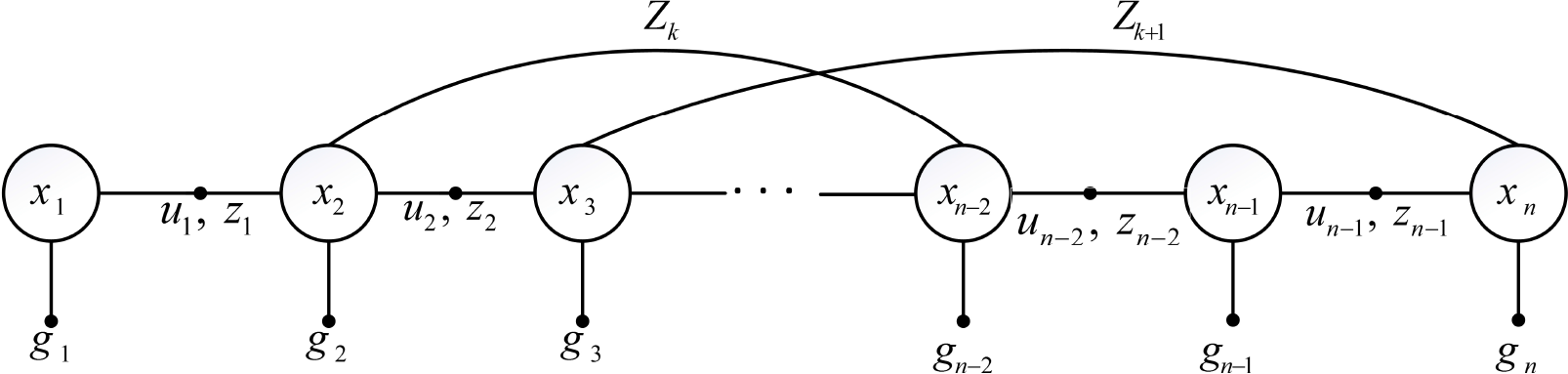
The pose graph of the SLAM problem constructed in the offline mapping process. Here, x i represents the vehicle's poses, u i represents inertial navigation measurements, z k represents lidar scan registration constraints in adjacent poses and loop closure poses, and g i represents the GPS prior constraints.
In light of the prior data containing the global positions from GPS, the velocities from inertial navigation and the measurements from lidar, we wish to construct a consistent representation of the real environment to put the measurements into their proper positions. We first construct a coarse pose graph with GPS global positions and lidar scan registration constraints. When there are nodes in the pose graph, which are spatially neighbouring but temporally separated, the nodes must be refined so that the measurements in the nodes can be matched properly. Briefly, the iSAM [14] is used to solve an optimization problem, in which adjacent nodes in the pose graph are linked by inertial navigation and scan registration, nodes are linked to their estimated global positions and the transformed error is distributed over the graph once the loop closure is detected.
In this implementation, we use the lidar odometry and mapping (LOAM) [32] algorithm to estimate six degrees of freedom scan registration constraints between adjacent nodes. Once a series of matches between both general nodes and loop closure nodes have been estimated, the iSAM objective function is minimized and the nodes, denoting the vehicle's poses, are updated accordingly.
Given the calibrated lidar intensities and the optimized vehicle's poses, the algorithm to build an average intensity map is straightforward. As the vehicle passes through the optimized poses, the lidar points are projected onto an x-y grid cell map, in which each cell represents a 20 cm × 20 cm patch of ground. When new lidar data arrive, each cell updates its intensity average combined with the stored necessary intermediate values. In this way, we build a highly accurate offline 2D prior map, shown in Fig. 2, to represent the known 3D environments.

The built highly accurate lidar intensity map. In (a), we show a 200m × 200m grid cell map, in which each cell shows its average intensity. (b) is a zoomed-in view of the red rectangular region A in (a), in which we can clearly see the stop lines at the crossroad. (c) shows a zoomed-in view of region B, where the lines of parking spaces can also be clearly seen.
3.3. Smooth local map
The construction of the local map needs to handle the current intensity readings in real time, which is an online task. As such, we cannot obtain the well-optimized vehicle's poses using the offline SLAM algorithm as per the last subsection. In addition, because of occlusions and/or multi-path reflections, the GPS positions can suddenly jump, such that the built map, which uses GPS to direct positions itself in relation to vehicle's poses, is ambiguous and will appear as a ghost. In contrast, the inertial measurements are smooth and invariant with GPS jumps. We integrate the inertial velocities to form a smooth coordinate system and build the local intensity map in this coordinate system.
The construction of the local map is similar to that of the prior map. Given the calibrated intensity readings and the accumulated vehicle's poses as a result of integrating the velocities, we project the current lidar points onto the 2D grid cell surface (z=0), with each cell representing a 20 cm × 20 cm patch of ground. Every cell stores the necessary intermediate data to update its intensity average with new readings falling into the cell. In this way, we create a smooth local 2D map to represent the current 3D scenes.
Since the smooth coordinate system is accumulated with time, its offset from the truth coordinate system gradually increases with the distance travelled, which limits the accuracy of the local map. Therefore, instead of the persistent integral from the start point of the path to the end point, we only integrate the velocities in a short period of time to maintain a short-term map. Once the vehicle's trajectory exceeds a certain range, the start point is reinitialized and the local map is reconstructed. In this way, it reduces the accumulated offset and ensures the accuracy of the local map.
3.4. The map's attributes
As the lidar point cloud is sparse, which is especially obvious in the region that is far away from the lidar, one characteristic of the built map is the uneven coverage. In the regions that are close to the vehicle's trajectories, the map is densely covered with lidar points, whereas, in the more distant regions, the map is sparse and with many irregular-shaped “holes” in it, as shown in Fig. 3. The gradients of the pixels in the holes vary dramatically, which results in severe disturbance for the construction of a robust feature descriptor based on the gradient; for example, the state-of-the-art SIFT [15] descriptor. Fig. 3(a) shows the results of one randomly selected SIFT point and its 50 most similar SIFT points in the map. The selected point is marked with a blue square with white number 1 as its label. The similar points are marked with red stars with green numbers as their labels, while the smaller the numbers, the more similar the descriptors.

(a) shows the results of one randomly selected SIFT feature point with white number 1 as its label and its 50 most similar ones with green numbers as their labels. The smaller the numbers, the more similar the descriptors. (b) shows the similarity scores of descriptors between point 1 and other points. (Due to the small size of the numbers, this figure is best view in colour and by zooming in.)
From Fig. 3(a), we can see that most of the points are located in the sparse region of the map and do not emanate from the special physical positions, as expected in the camera image, such as the intersections of the boundary of the objects and the corner points of the road markings. These feature points are unstable and susceptible to changes when new lidar data are accumulated into the map. This is an obvious difference between our generated map and the camera image. In addition, the similar descriptors should, ideally, represent similar regions; however, Fig. 3(a) shows that the region, which the selected feature point represents, is significantly different from the regions represented by its similar feature points. This indicates that the SIFT point descriptor in our low texture map does not have sufficient descriptive power. The similarity score between the selected SIFT point descriptor and its similar descriptors is plotted in Fig. 3(b). As these points denote dramatically different regions, their similarity score should ideally be distinguishable. In fact, as the ratios of the two adjacent similarities are in a range of [1.0007, 1.0426], they are so close. Such a small difference is not enough to distinguish the points.
Another characteristic of the map is its abundance of line segments, which consist of the 2D projections of buildings, the boundaries of different reflective attributes, the road markings and so on. Compared with lines in the camera-based image, these lines are immune from shadows and other artefacts caused by changes in lighting, as well as being stable because the buildings do not move, the reflective attributes of the objects do not vary and the road markings cannot disappear. The advantages of lines on the lidar intensity map make it a good option to match maps built at different times and under different environmental conditions. Thus, we firstly propose to adopt line segments to match the lidar intensity maps.
4. Line Segment Matching in Maps
In this section, we first depict the method to detect lines in the octave maps and construct the line band descriptor [17], which is a very efficient representation of the local appearances of lines. After considering the similar patterns of line pairs in the low texture map, we propose to combine the local appearance, the geometric attributes and the structural information collected through the lines’ neighbourhood to construct an affinity graph, as well as solve the matched problem using the spectral technique.
4.1. Line detection in the octave maps
It is well known that line segment detection in one low texture map may be broken into several fragments in another low texture map. To solve this problem, we downsample the original map with a series of scale factors and Gaussian blurring, after which we form a scale-space pyramid consisting of multi-layer maps. In each layer, we adopt the EDLines [34] algorithm to detect a series of line segments. To merge the lines from different scale-space maps, which are related to the same region in the original map with the same orientation, we find the corresponding lines in the scale-space maps, assign them a unique ID and store them in a vector called LineVec [17]. The final detection result is a series of LineVecs. Compared with the method [27], which stores all possible grouping lines, this method reduces the dimension of the line matching problem.
4.2. Line band descriptor
Given a detected line segment in the scale-space map, we use the line band descriptor (LBD) [17] to represent the local appearance of the line. The descriptor is computed from the line support region (LSR), which is a local rectangular region centred at the line. The LSR consists of a series of non-overlapping line bands, where each line band is parallel to the line, while its length is naturally equal to the length of the line segment.
Similar to MSLD [26], the line direction dL, which is defined as parallel to the line, along with the gradient of most of its edge points pointing from the left side to the right side, and the direction

where
Stacking the four accumulated gradient values of each row associated with the band, Bi forms the band descriptor matrix
4.3. Constructing the affinity graph
An affinity graph is built using the combination of three different kinds of information: appearance similarity, pairwise geometric attributes and structural likelihood. In this graph, the nodes represent the potential correspondences of matched lines, while the weight on the edges represents the pairwise agreements between them.
Appearance similarity is measured by the distance between the LBD descriptors. The distances between all descriptors of a LineVec in the prior map and a LineVec in the current map are computed, while the minimal descriptor distance is used to measure the pairwise line appearance similarity. The line pairs, whose similarities are less than a threshold, are taken as the candidate matches.
For a set of n candidate matches, the affinity graph is described with an adjacency matrix

In the typical environment, there are often similar patterns, for example, rows of buildings, and a series of equally spaced crossroads, so that the boundary lines extracted in similar regions of the map are too close to be distinguished. Fig. 4 shows an example of the generated map on the campus with four similar rectangle regions labelled with green letters (A, B, C and D). The red detected line 1 and line 2 have similar lengths, directions, descriptors and geometric attributes between the pairwise lines. To distinguish them, in this paper, we propose to add the neighbourhood structure to measure the geometric arrangement of the detected line segments. To describe the structure, the convex hull of every line neighbourhood is constructed as the smallest convex polygon, which consists of all the vertices of the neighbouring line segments, as well as the line itself. Examples of constructed convex hulls are shown in Fig. 4: the convex hull connected with the blue dotted lines is the constructed polygon of line 1 and its neighbouring lines; the convex hull connected with the yellow dashed lines is the constructed polygon of line 2 and its neighbouring lines. We can see that the two convex hulls reflect the neighbourhood structure of the lines and, fortunately, they are different.

The line's structural representation. The detected lines in the map, labelled with red colour, and four very similar regions, labelled with green letters (A, B, C and D). The polygon with its vertices connected with blue dotted lines is the constructed convex hull from line 1 and its neighbouring lines, while the polygon connected with yellow dashed lines is the constructed convex hull from line 2 and its neighbouring lines. This yellow polygon to the right of Fig.4 explains how to represent the area ratios matrix
We use the area ratios between the regions of the polygons, formed by connecting continuous vertices on the convex hull, to measure the structure likelihood. For line
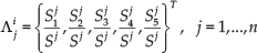
where
Supposing, for LineVec (

where

where
4.4. Problem-solving using the spectral technique
The line matching problem is now reduced to finding the cluster C, which maximizes the total consistent score

where x is subject to the mapping constraints, while the optimal solution
The general quadratic programming algorithms are too computationally complex to solve this problem. We relax both the mapping constraints and the binary constraints on x, such that its elements can take real values in [0, 1] and adopt the spectral technique to solve it. Based on the Raleigh's ratio theorem [16],
5. Estimating Initial Positions
Given the prior global map, the smooth current map and the result of line matching, the estimation of the vehicle's initial position is straightforward. For a matched line pair (

Ideally, one point can fix the vehicle's global position; however, due to inaccurate locations of line end points in the low texture maps, we model the probability density of the neighbourhood of the estimated position with a 2D Gaussian distribution

where the variance σ2 of the Gaussian distribution represents the uncertainty of the positions of the line end points, while (x, y) represent the neighbouring positions.
Given the probability of neighbouring positions, rather than directly using the centre of the probability distribution, which will tend to make the estimated position biased too much towards the centre, we use the centre of mass with enhanced probability with exponent

In this way, the initial guess about the position in the localization is obtained.
6. Experiments
We validate the performance of the algorithm proposed in this paper on the data from the campus, which are collected by the autonomous ground vehicle (AGV). The AGV is a modified Toyota Land Cruiser equipped with a Velodyne HDL-64E scanner, a NovAtel SPAN-CPT GPS-aided INS, cameras and laser range finders, which is shown in Fig. 5. We run the algorithm in C++ on a laptop equipped with a Core i7-2720 QM central processing unit (CPU) with 2.20 GHZ and 8 GB of main memory in Ubuntu. As the average runtime is 0.3s, we update the initial position for the localization module once every 0.3s.

Our testing platform is equipped with a Velodyne HDL-LIDAR 64E scanner (on top) and a combined GPS-aided INS (not visible)
6.1. Matching results in maps
The data used for building the prior map were collected by our AGV on a rainy day in May 2014, when a few vehicles were driving normally around our testing vehicle. Due to the effect of the rain on the road, the intensities of lidar reflectivity in these regions are dark, while the moving vehicles can also taint the map. Upon closer inspection, the trails from passing vehicles can be seen in the regions where there are some bright trajectories on the dark roads, as shown in the left column of Fig. 6. The data used for generating the smooth map were collected on a sunny day in August 2015. The lidar reflectivity represents its real attributes and the intensities are bright; meanwhile, given that there are only one or two vehicles passing, the map is relatively clean, as shown in the right column of Fig. 6.
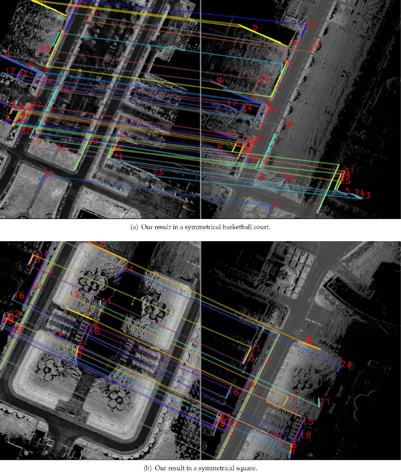
Matched results of our method in the symmetrical scenes. The red numbers are unique labels assigned to the corresponding lines; the lines in each pair are assigned the same colour, while one of their end points is connected to illustrate their correspondences. (The figure is best viewed in colour.)

Matched results of our method in the complicated scenes. The meanings of labels, lines and colours are the same as in Fig. 6. (The figure is best viewed in colour.)
To evaluate the performance of line matching in the low texture maps, we compare our algorithm with state-of-the art algorithms [30, 27, 17]. The compared algorithms are three representative ones, which are reported as producing excellent performances: namely, the line matching through line-point invariants [30] algorithm, the line signature [27] algorithm, and the LBD descriptor and geometric attributions [17] algorithm. The codes of the three algorithms are taken from their authors, while the parameter settings are recommended by the authors. All four methods are tested on the same computer, which is equipped with a Core i7-2720QM CPU with 2.20GHZ and 8 GB of main memory.
Given that the matched maps are built with lidar, the line matching in camera images is not within the scope of our interest. Thus, the experiments are only executed on the lidar intensity maps. We conduct the comparison experiments in four challenging scenes. As one experimental result of one algorithm in one scene consists of two images, the total results comprise 32 images. Owing to the limitation of the space, we only give the results of our algorithm, as shown in Fig. 6 and Fig. 7, while the statistical results of the four algorithms are given in Table 1. In Fig. 6, the left image is the prior map and the right image is the current map. The prior map is a complete representation of the scene, whereas the current map only represents a part of the scene, because the testing vehicle has not completely passed the scene. This is a great difference between the two maps. The vertical white line is the boundary of the two maps. The red numbers are unique labels assigned to the corresponding lines, with the lines in each pair assigned the same colour, while one of their end points is connected with the respective colour to illustrate their correspondences. The correctness of the matches is judged visually.

In Fig. 6(a) and (b), the results of our algorithm in two symmetrical scenes are shown, in which the prior map is on the symmetry of a line and the current map occupies nearly half of the prior map. The method [30] only matches three line pairs in all, which means that it is less suitable for the low texture map because the local appearances of lines are indistinguishable, while the maps lack stable key point correspondences. (Although [30] uses SIFT feature points to construct line-point invariants, SIFT points are very similar in the lidar map; please refer to our analysis in Section 3.4.) In addition, the runtime is minute-level; the reason lies in the fact that it extracts large numbers of SIFT feature points (more than 6,000) and constructs line-point invariants based on these feature points. In contrast to [30], the method [27] is superior because it exploits spatial geometric configuration to measure line pairs. The runtime is second-level; it needs to construct a large number of computationally complex line signatures. The method [17], which is based on new LBD descriptor and pairwise geometric attributions, is more superior, while the run time is millisecond-level, which means the drawback lies in its match precision needs, which must be improved further. In contrast to [17], our method, which considers the structural information, improves the match precision with slightly increasing the runtime.
In Fig.7(a), there are five almost identical regions in the prior map, while the extracted lines in these regions are hard to distinguish, which results in a relatively low match precision in [17]. Similarly, the complicated multi-crossroads map in Fig. 7(b) also reduces the match precision in [17]. Our method also improves the match precision in the two scenes.
6.2. Estimation of initial position
We test the performance of the initial position estimation algorithm proposed in this paper in two closed campus scenes. Fig. 8(a) shows the results around a basketball court; the green points are obtained by directly projecting the current GPS positions onto the prior map, which has been built in advance using the offline SLAM technique. Ideally, they should fall in the proper positions of the prior map; however, when the GPS signal is occluded by big trees and/or high buildings, the GPS positions may undergo a drift or severe jumps, such the projections fall wrongly into the obstacle regions. The blue points are the projections of the integrated positions. From Fig. 9(a), we can see that the trajectory of the GPS fits well with the integrated one, which indicates that the velocities are stable and the GPS positions do not jump. However, the two trajectories are both off the road, which indicates that the GPS positions have drifted. Through manual measuring, the drift reaches 16m. The red points are the estimated positions using our method, with the majority of points falling orthographically on the road.

Estimated initial positions in two closed environments. The green, blue and red points denote the projections in the prior map of the current GPS readings, the positions of the integral over velocities and our estimated initial positions, respectively. Better results should have more points falling in the proper positions on the road and have smaller closed errors. (The figure is best viewed in colour.)
Fig. 9(b) shows the results around a swimming pool. Upon closer inspection, the green GPS happens to jump drastically in the top right of the map, after which the total trajectory produces a severe drift, finally resulting in an error of more than 80m in the end point of the test, which should have been closed. The blue integrated positions have drifted dramatically since the first turning in the top of the trajectory, while the points located within the two turnings in the top fall fully into the obstacle area, which is about 20m away from the road. The final error between the start point and end point is about 24m. The red trajectory is the estimated result of our method; there are only a few points deviating from the road in the top left of the trajectory, as most of them are located in the orthographic positions. The start point and the end point are well closed. The qualitative tests confirm that our algorithm can effectively tackle the sudden jump in a GPS signal, thereby providing a reliable initial value for subsequent precise localization.

Histograms of longitudinal and lateral errors produced by our initial position estimation algorithm. Large errors are caused by the inaccurate locations of line end points, which are intrinsic to line detection.
We adopt the strategy of local odometry to quantitatively evaluate the performance of our method. The ground truth is obtained by optimizing the vehicle's current poses in the closed trajectory using the SLAM method [14], with the lidar scan-matching [32] providing constraints and the start point being set as (0, 0). This strategy not only eliminates the drift of the initial position and the sudden jump in the GPS signal, but also removes the accumulated error. The global coordinates are converted into the local ones by subtracting the start position. Thus, the ground truth and our results are in the same coordinate system. We present longitudinal and lateral errors in histogram form in Fig. 9. From the figure, we can see that the longitudinal error is concentrated within 3.5m of the ground truth, with the mean error being 1.68m, while the lateral error is bounded in the range of 2.5m with the mean error being 1.04m.
7. Conclusions
The initial position estimate in lidar intensity maps can be difficult because such maps have these characteristics: low contrast, great gradient changes in the sparse regions and rich similar patterns. In this paper, we propose an algorithm to estimate the initial position of an autonomous vehicle by matching line segments in maps. The maps consist of a highly accurate prior map, built with the offline SLAM technique, and a smooth current map, built with the integral over velocities from an INS. To measure the pairwise consistency, we propose adopting the local appearance, pairwise geometric attributes and structural likelihood in order to construct an affinity graph for the candidate line matches, and employing a spectral technique to solve the matching problem efficiently. The initial position estimate is obtained according to the relationship between matched lines and the vehicle's position. Experiments on campus, with GPS error of a few tens of metres, show that our algorithm will always provide an accurate initial position with metre-level accuracy, which can meet the needs of the initial guess in the localization.