
Abstract
Robotic air vehicles are used increasingly in delivering goods especially for safety-of-life applications. This paper discusses a guidance module for trajectory generation of such vehicles. An offline algorithm is developed using a navigation model to produce the required trajectory in the form of time-tagged longitude, latitude and altitude. The process is an essential requirement when an operator has to program a robotic vehicle to travel on the desired course. This problem is addressed scarcely in the relevant literature.
The waypoints are generated for all phases of flight and then modified to cater for the wind disturbance parameters obtained from current meteorological information. The waypoints are uploaded to the vehicle's flight control system memory and reside there for the vehicle to follow. This paper also renders the generated trajectory on Google Earth® using Matlab/Simulink® to test the closed-loop performance. Furthermore, a Dryden wind model is utilized to generate a modified trajectory for turbulent conditions. An operator can make adjustments in the required initial heading angle so the vehicle lands at its destination even in turbulent weather. An empirical formula is also proposed for this purpose. Further work includes design of a control system to follow the generated waypoints.
1. Introduction
With the rapid improvements in aerospace technology, intelligent Unmanned Aerial Systems (UAS) are playing an instrumental role in providing help and guidance not only in military but also civilian applications. Safety of life (SOL), delivery of emergency aid and high-value products are key markets for such systems in the civil domain. The future dominance of UAVs has been indicated by companies like Amazon, which has introduced Prime Air drones for delivery of packages to its customers.
Execution of completely autonomous flight needs gate-to-gate trajectory generation by the guidance system. Most of the algorithms and schemes discussed in the literature focus on level flight, though some do address the take-off and landing issues. However, gate-to-gate autonomous flight is rarely addressed. In common literature, consideration is given to optimization of level flight where detailed flight plan parameters are not addressed [18]. Moon and Kim [11] do propose a 3D trajectory generation; however, the time at which the vehicle should pass through each of these waypoints is not included in their trajectory model. Lin and Tsai [19] derive analytical solutions for a closed-loop nonlinear optimal guidance law for three-dimensional mid-course and terminal guidance phases. Rao [16] improves these analytical solutions by dealing with nonlinear terms that were neglected by Lin and Tsai. Choi, Curry and Elkaim [6] present two path-planning algorithms based on Bezier curves for autonomous vehicles with waypoint and corridor constraints. The trajectory generation problem has also been solved by optimal control techniques [9,29]. Chebyshev pseudo-spectral approximation [21, 23] has been presented as an improved polynomial approximation method, using a Runge-Kutta scheme [28] or collocation methods [26] in the sense of Chebyshev norm where the derivatives of the approximating polynomials are exactly known; previous approaches resorted to derivative approximations. Some others address the issues of correct guidance during turbulence [19]. However, even when wind turbulence and trajectory optimization are considered, all flight domains are not addressed [21]. The methods mentioned so far deal with 3D or 2D waypoint-based trajectory and some specific portion of the autonomous flight. The present work deals with the 4D navigation trajectory generation for a complete gate-to-gate autonomous flight, which will reduce uncertainty and increase predictability for both air-traffic service users and providers. Important contributions of this paper are presentation of a structured gate-to-gate trajectory generator including demanding phases of take-off and landing, an interface with open-source flight simulation software, use of a wind model to cater for disturbances, and suggestions for practical implementation of a UAV-based trajectory correction system.
A fully automatic air vehicle needs to have three primary modules in the on-board computer; these are the guidance, navigation and control modules [7]. As the guidance module is responsible for generation of detailed point-to-point commands for the flight control system in light of the defined mission and current flight data obtained from the navigation module, in this paper, the algorithms for this guidance module are discussed for gate-to-gate autonomous flight. This procedure is followed until the aircraft reaches its destination. This paper uses a navigation model that updates its state vector to generate a trajectory consisting of waypoints from the starting point to the destination. Rhumb-line steering is adopted for the navigation path after comparison with great circle steering [14]. The former method is selected because it only generates a single heading value to be followed throughout the trajectory. This is a significant advantage in performing optimal operation of the vehicle. However, these methods provide parameters for cruise flight only. For gate-to-gate operation, waypoints are to be generated for all phases of the flight. The algorithm discussed in this paper does this job for all the phases including take-off, climb, level flight (or cruise), accelerated flight, decelerated flight, landing, and turning of the aircraft. Hence, it provides a realistic picture of operating an autonomous vehicle.
Although real flight tests have their own significance, simulation-based verification has been adopted in this paper. The reason is that flight simulation tools are now sufficiently mature and precise; moreover they save time, cost and effort. This paper therefore demonstrates flight verification using FlightGear®, which is an open-source advanced flight simulator. FlightGear® provides the closest available graphics platform to the real world [12]. Google Earth® has been used to visualize all the waypoints.
In order to simulate in FlightGear®, this paper generates results for a sample trajectory from San Francisco International Airport to San Carlos Airport, United States. Once the waypoints have been generated according to the complete flight plan, they are passed to the Simulink model. This Simulink model starts simulation with simultaneous execution of the FlightGear® software. The results are shown in the form of snapshots of the running simulation. Apart from this, graphs for different trajectory parameters are also given. The results show the accuracy of waypoint guidance from take-off to landing, hence validating the algorithm for use in actual flights.
Section 2 outlines a simplified architecture of the guidance algorithm that is used to generate the required trajectories. In section 3, the mathematical model implemented in the waypoint guidance algorithm is explained. Section 4 presents a case study to show the usefulness of the discussed algorithm. The trajectory generated according to the parameters discussed in the case study is then validated in Google Earth® in section 5. Section 6 presents the FlightGear® simulation and results. Brief information is also given regarding the FlightGear® simulator and the interface of Simulink® with FlightGear®. The trajectory generated in Matlab® is validated through the successful flight simulation in FlightGear®. Detailed simulation results are presented. The paper ends with a brief conclusion and useful references.
2. Simplified Guidance Algorithm Structure
An aircraft flies according to a flight plan which summarizes the desired flight navigation parameters from starting point to the destination. The flight is divided into different phases and each phase has waypoints for an automatic vehicle to follow. A guidance algorithm generates all these different waypoints and a control algorithm tries to follow them through manipulating the vehicle's actuators (its control surfaces and throttle) [25]. The present waypoint guidance algorithm is divided into different subroutines which are called as the aircraft flies through different phases, as shown in the flowchart in Figure 1.

Simplified architecture of the proposed guidance algorithm
As shown in this figure, the guidance algorithm has the main body that takes parameters from a flight plan and decides to use subsequent routines based on the trajectory requirement. As required by the trajectory, the aircraft needs to accelerate, decelerate or turn. The waypoints are appropriately selected so as to facilitate these manoeuvres. A trial-and-error procedure is adopted to fine-tune these parameters. Once the trajectory is generated it is validated by using Google Earth® and FlightGear® software. The mathematical model required for the generation of trajectory is described in the next section.
3. Mathematical Model
Generally, there are two types of motion planning: deliberative and reactive [7]. Reactive motion planning uses behavioural methods to react to local sensor information, which are well suited for dynamic environments, particularly in collision avoidance, where information is incomplete and uncertain; however, it lacks the ability to specify and direct motion plans. This paper adopts deliberative planning, in which all the trajectories to be followed by the vehicle are decided pre-flight based on the calculations using the knowledge of earth. Deliberative motion techniques have been found to be effective and efficient for miniature air vehicles in approaches where trajectories are planned explicitly. In waypoint navigation, two types of steering method are typically used: rhumb-line steering and great circle steering [14]. Though these methods are old, they still provide effective solutions for trajectory generation. They are very briefly described next.
3.1. Rhumb-line steering
In this steering method the aircraft implements a constant bearing or heading until it reaches its final point for that part of the trajectory. The algorithm for rhumb-line steering is derived from the following basic set of equations:

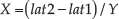


where (lat1, lon 1) and (lat2, lon2) are the initial and final points of a specific portion of the trajectory, Y and X are the intermediate variables used for calculating the loxodromes (i.e., rhumb line – an arc crossing all the longitudinal meridians at the same angle). Courses and distances are calculated according to the definitions below.
Course gives the true bearing between the initial and final points of the trajectory segment. Distance gives the true rhumb-line distance between the two points.
Latitude is used to calculate the geodetic latitude of the waypoints after the aircraft has travelled a specific distance from the initial point.
Longitude is used to calculate the longitude of the waypoint on a true course after the vehicle has travelled some distance along the rhumb line.
3.2. Great circle steering
A great circle is any circle whose centre coincides with the centre of the earth while its radius equals that of the earth. The trajectory follows the path of the great circle between any two points. The algorithm is derived from the following basic set of equations:


where
3.3. Navigation model
The position of the aircraft is determined by latitude, longitude and height, while for navigation, the component form of the velocity is used. The model described here represents the updating of the navigation state vector. This state vector contains the position, velocity and attitude of the vehicle. The algorithm for the waypoint guidance module is derived from the following basic set of equations [4]:


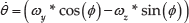
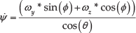
where
To implement the algorithm described above, values for specific forces for accelerometers and angular for gyros are required (specific force is a term that denotes output of an accelerometer). These are indicators of the forces and torques on an aircraft during flight [22]. Once estimated values for these are plugged in, the velocity vector is calculated. For uniform velocity, initial and final velocities are equal, but they are different in the case of accelerating/decelerating flight. Similarly, for turn trajectory, a turn rate is assumed between the initial waypoint and the final waypoint of a turn. This procedure needs to be repeated until the data generated for velocity and angles are finalized and provide smooth transitions in the generated trajectory. Hence, after the application of this algorithm, a full data set for a typical trajectory is generated and is ready to be used for guiding an automatic vehicle. A case study is described next to show the usefulness of the discussed algorithm.
4. Trajectory Specifications
In order to simulate the algorithm results in FlightGear®, this paper shows the waypoints generated for a sample trajectory in the virtual environment from San Francisco International Airport (KSFO – runway 10L) to San Carlos Airport (KSQL – runway 30), United States. The details are shown in Table 1. The output of the trajectory algorithm are point-to-point flight data for position, velocity and attitude of the flight vehicle. These data are needed to steer the aircraft from the source to the destination by a control algorithm. The data are then validated in Google Earth to ascertain whether they are appropriate for the specific trajectory.
Sample data generated for airports of San Francisco and San Carlos, USA

5. Trajectory Validation in Google Earth®
The waypoints generated are first validated by interfacing the Matlab software with Google Earth®. Figures 2, 3 and 4 display the trajectory according to the complete flight plan. From visual inspection it can be seen that a reasonable model for the trajectory has indeed been generated.
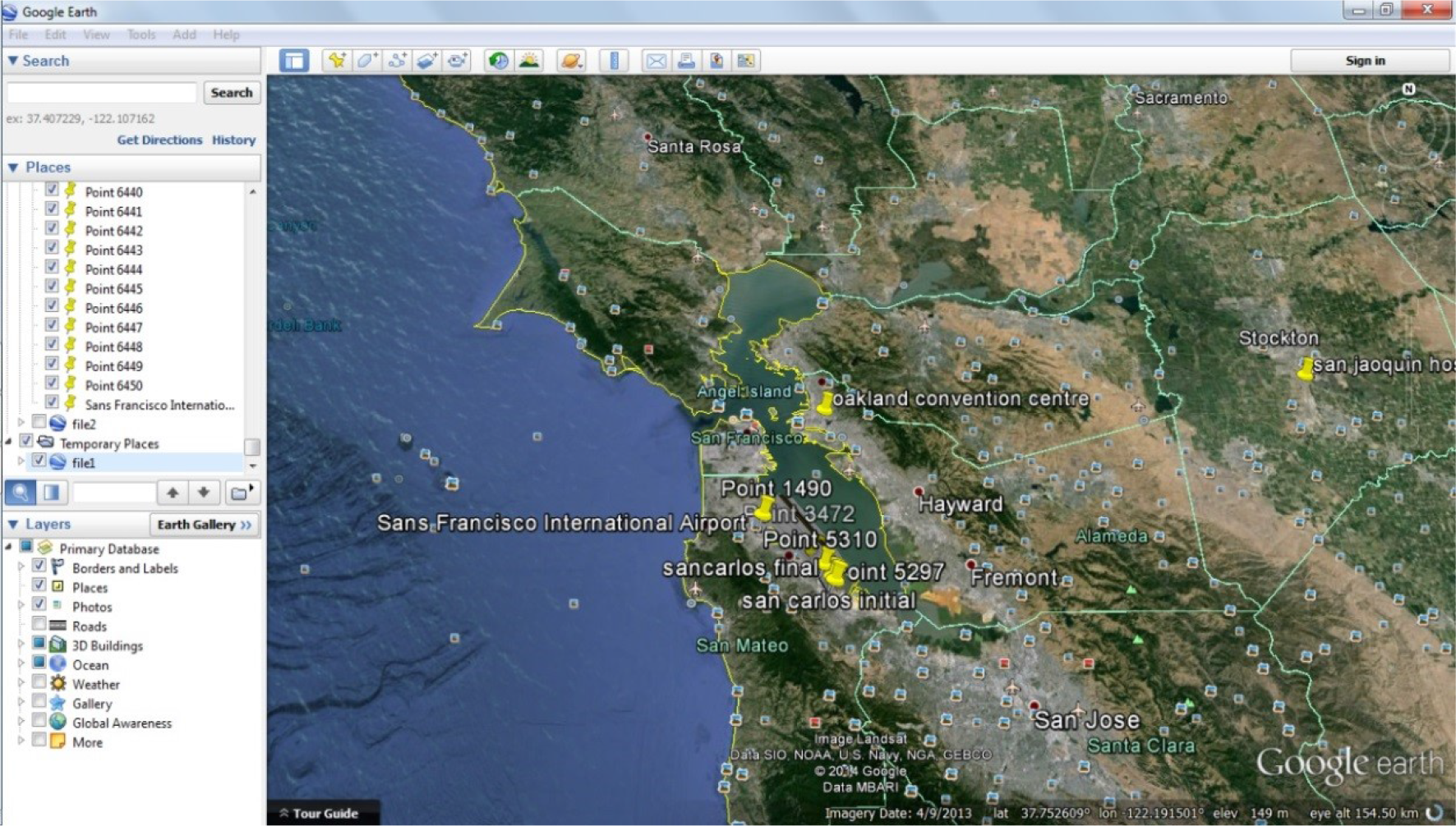
Trajectory between the two selected airports
Once it is established that the trajectory is complete for all the phases of flight, it can be checked using flight simulation softwares. A good choice is the open-source flight simulation software FlightGear® that has the capability of simulating high-quality flight for a number of aircraft models [12]. Its usage is described in the next section.

Waypoints in the generated trajectory

3D view showing ascent and descent of the aircraft
6. FlightGear® Simulation And Results
6.1. FlightGear® simulator
FlightGear® is an open-source flight simulator designed to be used for research or pilot training or as a professional engineering tool. FlightGear® has its own simulation engine called SimGear and also provides a wide range of aircraft models to be selected for simulated flight. The terrain engine, called TerraGear, provides different weather effects that include 3D clouds, lighting effects and time of day. The main feature of FlightGear® is its dynamic model, which consists of UIUC, YAsim or JSBsim. [12] These three are basically models based on different calculation methods which determine how the flight for an aircraft is simulated in the program. In this paper, FlightGear® is interfaced with Matlab® to achieve a realistic simulation for the generated trajectory [13].
6.2. FlightGear® interface with Matlab
The trajectory generated in workspace of Matlab® is interfaced with FlightGear® through a Simulink® model. Waypoint positions are defined by the geodetic latitude, longitude and height while attitude is designated in the form of Euler angles.
Figure 5 shows the interface between the Simulink® model and FlightGear® software. This is a unidirectional transmission link from the Simulink® interface to FlightGear® using the “net_fdm” binary data exchange protocol [9, 10]. The UDP network packets are transmitted to a simultaneously running simulation of FlightGear®.
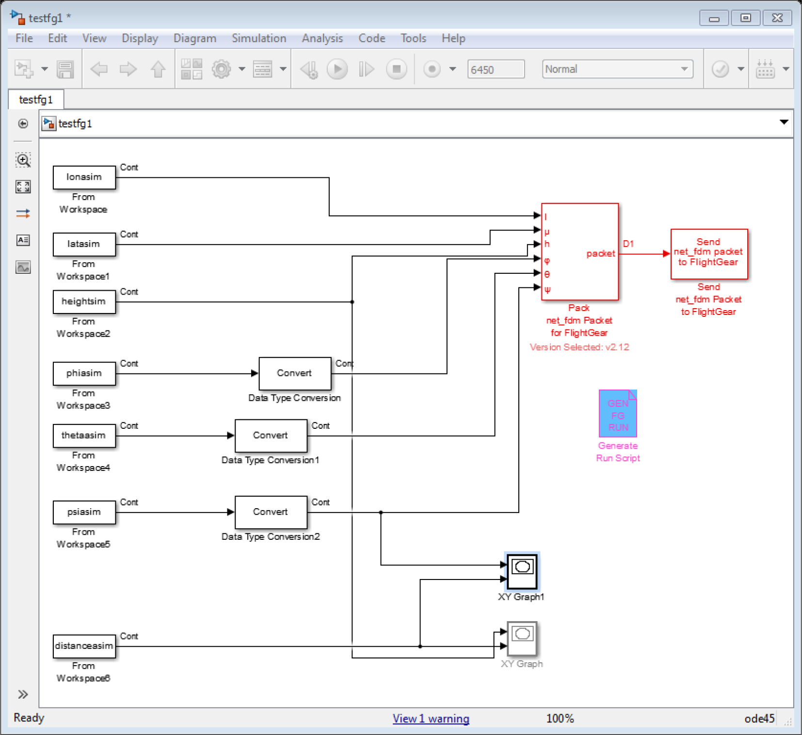
Simulink model
6.3. Trajectory validation in FlightGear®
The Piper J3 cub aircraft model is used in the simulation since its flight dynamics are most similar to that of a simple UAV. Real-time plots are also generated. The first plot in Figures 6 and 7 shows the relation between distance (m) and height (m) while the second plot shows the relation between distance (m) and heading (deg). It is to be noted that Figure 6 is drawn during the middle phase of flight and Figure 7 shows the landing part.
6.4. Results and discussion
The FlightGear® simulations validated the accuracy of the guidance algorithm since the aircraft completed all its phases of flight according to the generated trajectory. The following figures illustrate the relation between some of the variables defining the trajectory.
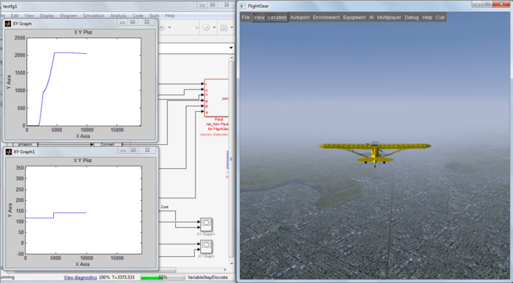
En-route phase in FlightGear®

Landing phase in FlightGear®
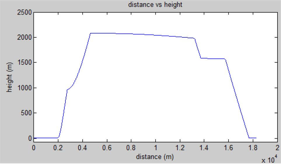
The comparison between the longitude and latitude travelled by the aircraft model is shown in Figure 8. Figure 9 displays the relation between the distance travelled and height achieved while going through the different phases of flight. It can be noted that the aircraft flies at about 2 km altitude while cruising and covers about 18 km in distance while travelling between the two airports.
The change in heading along different longitudes is shown in Figure 10. Figure 11 portrays the comparison between longitude and horizontal velocity of the aircraft. The algorithm results also showed that there is only a minute difference in the two types of steering based on the distance covered. However, as the distance is increased, the difference between them also increases, as great circle steering is the shortest path between any two points on the earth. However, it has the drawback of having a continuously changing heading angle, which is kept constant in rhumb-line steering.
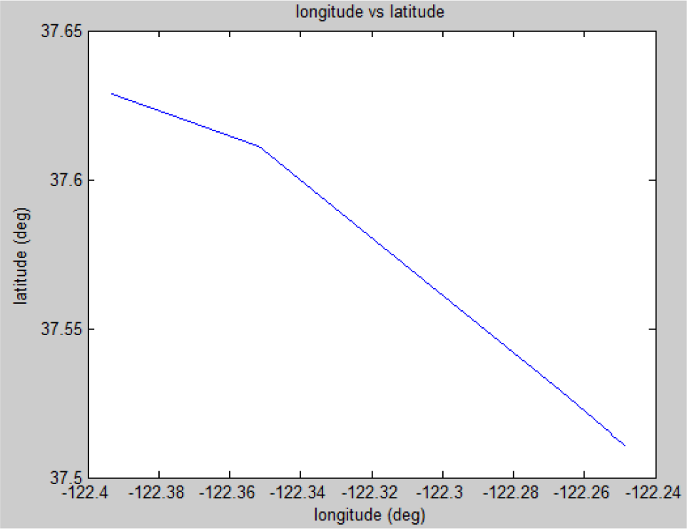
Longitude vs Latitude
Longitude vs latitude
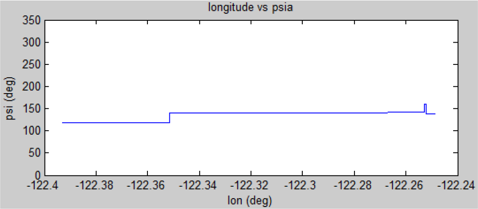
Longitude vs Heading

Longitude vs horizontal velocity
Once a trajectory between two points is generated, a practical obstacle is to include effects of weather. This is necessary since the operations of the aircraft need to be completed even in the presence of turbulence. The next step after initial trajectory validation is to introduce a turbulence model to ascertain effects on trajectory. The Dryden model for gusts is chosen, an old but popular model [15, 17] which provides easy implementation in Matlab®. In the Dryden model, gusts are treated as linear and angular velocity components; these components originate from rational power spectral densities [27]. It is possible to design exact filters that take white noise as input and generate stochastic process for use as turbulence forces and torques [30]. Figure 12 shows the incorporation of the Dryden model in the simulation developed in this paper to study the effect of turbulence on the generated trajectory.

Incorporation of Dryden model in the developed simulation
It can be seen that the Dryden model is used to generate linear and angular velocities that are seamlessly integrated with the developed model. In the figure,
As can be inferred from Figures 13 and 14, the two trajectories are generated using different heading, altitude, distance covered and waypoints. As mentioned earlier, this is possible because of the difference in flight plans of the two trajectories. The blue line represents one trajectory and the green line represents the alternative trajectory; the effects of wind on both the trajectories are shown by red lines.
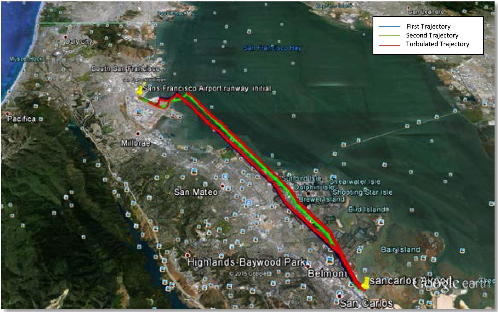
Complete trajectories and their wind effects
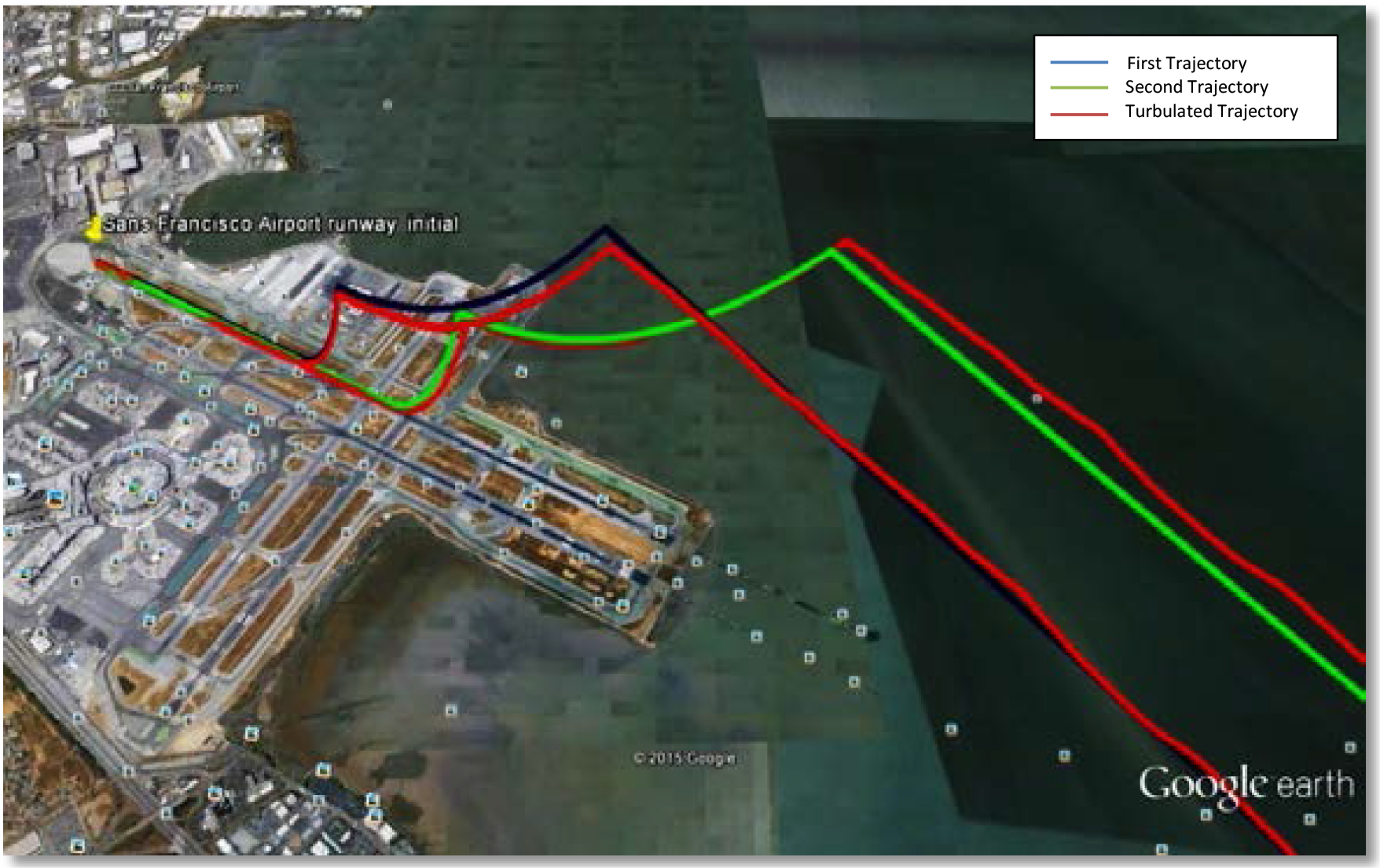
Take off and wind effects of both Trajectories

Initial and final approach of both trajectories

Landing and taxi of both trajectories
It can be concluded by analysing Figures 14, 15 and 16 that the first trajectory (green line) is more affected by wind compared to the new trajectory (blue line). In Figure 17, the Euler angles of second trajectory and its wind effects are plotted.

Euler angles of second trajectory and wind effects
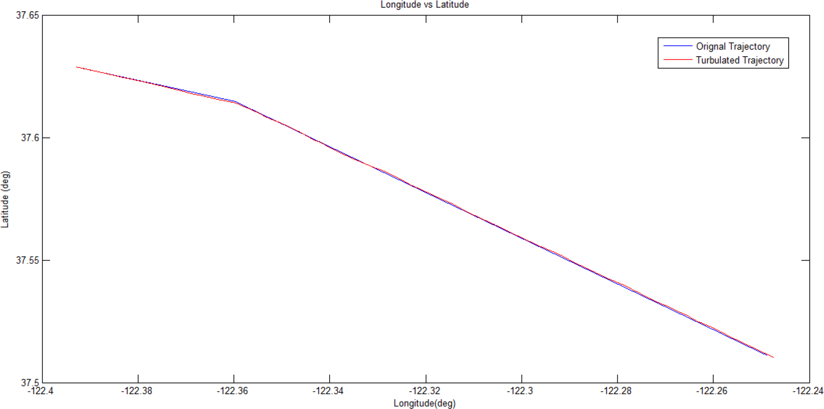
Latitude vs. longitude of second trajectory with wind effects

Horizontal velocity and longitude

Height vs. distance for second trajectory
Figures 18, 19 and 20 show various important parameters for the second trajectory – latitude, longitude, horizontal velocity, height and distance – and comparisons between them.
To quantify the analysis, Table 2 is generated. This table contains the variations in the two trajectories due to wind effects. It can be clearly seen that heading, latitude and longitude are all disturbed due to turbulence.
An effective method is to use the absolute difference column as a guide and add a bias value to it, in order to make the final absolute difference zero. For example, subtracting 6.5404 degrees from the initial heading of the first trajectory and 1.7369 from the initial heading of the second trajectory will ensure that final heading is the required heading.
The analysis in this table indicates that an empirical formula for initial heading adjustment can be coined to ensure a correction in the final heading. For this purpose, it is assumed that absolute difference in the heading due to wind turbulence is a Gaussian variable. This assumption is valid in general if a large population of errors is assumed. In this case, a variable follows Gaussian distribution and its value hovers within three standard deviations around its mean value 99.7% of the time [31]. To cover almost all the possible values of the random absolute heading difference, the following formula is suggested:
where ζi is the initial heading calculated by the rhumb-line steering formula, ζ A.D is the absolute difference in heading between the initial heading of benign trajectory and the trajectory with turbulent weather conditions, and ζc is the corrected heading. In the above formula, according to the Gaussian assumption (normal distribution of error) it is ensured that the correction will be able to cover approximately 90% of the cases as given by the probability density function of a normally distributed random variable with expected value μ and variance σ2:

Comparison of the two trajectories in terms of heading, latitude and longitude

Using current meteorological parameters that can be obtained daily from the Met department in the Dryden model, the trajectory can be fine-tuned before the start of the flight.
7. Conclusion
In this paper, a navigation model is used for trajectory generation of a robotic air vehicle. This trajectory contains complete gate-to-gate data from the taxi to the landing phase. Once the data are generated, these are validated by drawing 3D maps. Further verification is performed using the open-source flight animation/simulation software FlightGear®. The results show that this trajectory can be used with confidence for a real flight of a robotic air vehicle. The performance of trajectory generation is also tested using a turbulence model. In the case of trajectory generation for turbulent weather conditions a method is provided to ensure safety of flight operation. The solution is to generate the modified trajectory and adjust the initial heading so that the final waypoint is maintained as the original destination. An empirical formula is derived based on the generated trajectory data. The generated waypoint data will be used as set points for the control routine. Further work can be done to check the performance of the trajectory generator in the presence of wind models other than the Dryden model and to design a realistic control law. Another future direction is to include detailed dynamics of the aircraft so as to smoothen the rapid changes in the trajectory.
Footnotes
8. Acknowledgements
This project was funded by the National Plan for Science, Technology and Innovation (MAARIFAH) – King Abdulaziz City for Science and Technology - the Kingdom of Saudi Arabia – award number (11-SPA2059-03). The authors also acknowledge with thanks Science and Technology Unit, King Abdulaziz University for technical support.