Research on pure azimuth passive positioning of unmanned aerial vehicle formation in electromagnetic silence environment

Abstract

In the electromagnetic silence environment, for the azimuth-only passive localization problem in the conical formation, it was concluded that there was a deviation between the ideal standard formation and the actual formation. These disturbance deviations should be eliminated to make the UAV reach the ideal formation state. Therefore, the adjustment model of individual UAV, the directed graph model of formation node and the MDP model of adjustment strategy are constructed. Based on the relevant factor model constructed, the azimuth-only passive localization model in conical formation is established and solved in MATLAB. Finally, experiments and analysis are carried out in the simulation environment, and the effectiveness and feasibility of the proposed algorithm are proved.

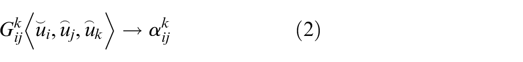
Introduction

In order to avoid external interference, unmanned aerial vehicle (UAV) swarms should keep electromagnetic silence as much as possible and emit less electromagnetic wave signals when performing formation flight.^1–7 In order to maintain the formation, a azimuth-only passive positioning method is proposed to adjust the position of the UAV.^8–12

The relationship between the position and the relative position in the cluster is established by only relying on the measurement information of the UAV’s own sensors and the relative measurement information inside the cluster. That is, a few UAVs in the formation transmit signals and the rest of the UAVs passively receive signals, and the direction information is extracted for positioning to adjust the position of the UAV.^13–15 Each UAV in the formation has a fixed number, and the relative position relationship with other UAVs in the formation remains unchanged.^16–18

Trujillo et al. proposed to combine monocular Simultaneous localization and mapping (SLAM) and multi-UAV information in a collaborative way to improve the navigation ability in GPS-limited environments. ¹⁹ Yun et al. have implemented a GPS-free vision-aided clustering localization method, in which the UAV swarm is equipped with laser ranging radar and all-weather vision system for positioning. ²⁰ Qin et al. carried out research on the UAV navigation system based on the fusion of vision and inertia, and carried out flight tests in an indoor environment. ²¹ However, in the practical application of UAV formation passive localization method, it is limited by many application scenarios. For example, vision-based localization methods have limitations such as limited camera perspective, easy to be occluded, and greatly affected by illumination. ²² Visual SLAM methods have poor effects in environments such as open venues and corridors with repeated features, and as resource-intensive algorithms, they need to run on high-computing units. ²³ Wireless range-based relative localization algorithms, such as Multidimensional Scaling (MDS) method, Extended Kalman Filter (EKF) method, The fusion localization algorithm of INS and wireless ranging based on EKF also has problems such as difficulty in determining the physical meaning of the coordinate system and easy divergence of positioning errors. ²⁴

The cooperative interaction ability of these UAVs is a critical factor that determines the success of their missions. To ensure effective operation in complex environments, there is an imperative need to develop a robust and reliable localization algorithm for UAV formations. This algorithm should be designed to minimize the use of radio communication, thereby maintaining radio silence as much as possible, which is crucial for stealth operations and avoiding detection by adversaries. It should also provide robust support for the cooperative control of individual cluster nodes within the formation, ensuring that they can effectively communicate and coordinate with each other without compromising their position or the integrity of the formation. Furthermore, the algorithm must be capable of maintaining the formation configuration even in the face of unexpected challenges such as environmental disturbances or equipment malfunctions. The development of such an algorithm would significantly enhance the resilience and adaptability of UAV formations, enabling them to perform a wide range of tasks with a high degree of precision and reliability.^25,26

In this paper, an adjustment strategy based on MDP model is designed to solve the problem of azimuth-only passive localization in conical formation in electromagnetic silence environment. Firstly, by constructing individual UAV adjustment model and formation node directed graph model, it is found that there is a deviation between the ideal standard formation and the actual formation. Based on the relevant factor model, the azimuth-only passive localization model in conical suiting formation is established and solved in MATLAB.

Azimuth-only passive positioning in conical formation

Problem analysis

This paper considers the azimuth-only passive localization problem of unmanned aerial vehicle (UAV) in different cluster formation modes. Due to the change of formation, the circular formation algorithm model cannot be applied to the new formation mode. Taking the cone-shaped UAV formation as an example, the distance between each UAV and its neighbors in the cone-shaped formation is the same, which is 50 m. The final formation of the formation can be determined. However, all the UAVs in the formation do not have accurate self-positioning (i.e. the UAVs themselves are not sure whether there is deviation), and the UAVs transmitting signals only provide the azimuth angle without the positioning and numbering information. When the position of an unknown number of UAVs is slightly deviated at the initial time, how to adjust the overall formation to achieve the ideal position only through the direction information received by the individuals in the formation. Making each UAV return to its own position in the formation is the main problem to be solved in the design of the adjustment scheme.

The establishment of the relevant factor model

Individual UAV adjustment model

In the formation scheme, the ideal formation is a conical formation. However, due to the existence of disturbance, the UAV cannot find its precise position in the formation, and there is a small position deviation.

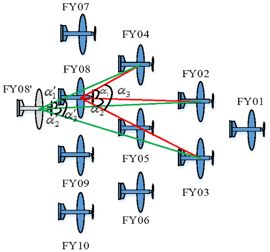
As shown in Figure 1, the precise position of individual UAV FY08 is shown in blue, and the angle information of FY02, FY03 and FY04 UAV in the formation that it can receive is ${\alpha }_1$ , ${\alpha }_2$ , and ${\alpha }_3$ , respectively. But in the case of small errors, it is shifted to the position of gray FY08′, after offset, the angle information of FY02, FY03, and FY04 UAV in the formation that can be received is ${\alpha }_1\prime$ , ${\alpha }_2\prime$ , and ${\alpha }_3\prime$ , respectively.

Figure 1.

Adjustment of individual UAVs.

Because there is a certain position difference between the actual UAV position FY08’ and the ideal UAV position FY08 in the plane, this position difference can only be adjusted by obtaining the azimuth information of the other UAVs, and the formation adjustment strategy needs to be converted from the plane position to the given angle strategy. Therefore, we construct the “phase angle” model. That is, the control force model that guides the UAV to fly to the ideal formation node is constructed by the difference of the relative angle. The principle is shown in the Figure 2.

Figure 2.

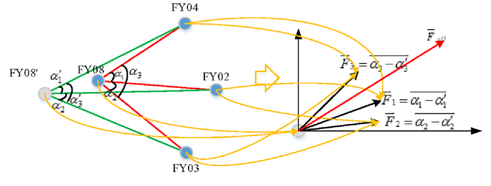
Schematic diagram of phase angle force.

UAV FY08’ needs to be close to its ideal formation position FY08, the angle information it receives and the angle information of the standard position are transformed into the phase angle force vector, as shown in the Figure 2. The three phase angle forces it is subjected to are:

$$\{\begin{array}{c}{\overrightarrow{F}}_1=\overrightarrow{{\alpha }_1-{\alpha }_1\prime }\hfill \\ \multicolumn{1}{c}{{\overrightarrow{F}}_2=\overrightarrow{{\alpha }_2-{\alpha }_2\prime }}\\ \multicolumn{1}{c}{{\overrightarrow{F}}_3=\overrightarrow{{\alpha }_3-{\alpha }_3\prime }}\end{array}$$

(1)

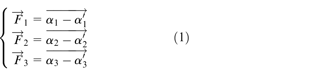
UAV FY08′ receives the phase angle force vector of the angle between each pair of the sending signal UAVs, and all the phase angle force vectors are superimposed to form a resultant force ${\overrightarrow{F}}_{\mathrm{all}}={\overrightarrow{F}}_1+{\overrightarrow{F}}_2+{\overrightarrow{F}}_3$ to guide it to fly to the standard position, so as to adjust the UAV individual and make it fly toward the standard node in the formation.

The formation node directed graph model

Intuitively, a directed graph is a graph of “nodes” connected to “edges,” where each edge is directed and represents an ordered pair between two nodes. In the whole UAV formation system, the individual UAV is regarded as the node, and the directed edge $〈u_i,j_i〉$ directs from the UAV $u_i$ which sends the signal to the UAV $u_j$ which receives the signal.

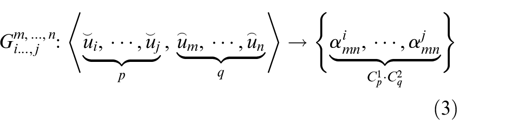
The directed graph we need is not the directed edge based on the node, but the angle formed from the signal sending UAV to the signal receiving UAV. Drawing on the idea of “node” and “edge” of directed graph, we can construct the directed graph model of formation node based on “node”, “edge,” and “angle” formed by UAVs considering sending and receiving signals, and its schematic diagram is shown in Figure 3.

Figure 3.

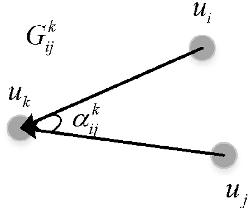
“Node” and “edge” of directed graph.

In the directed graph $G_{\mathrm{ij}}^k$ , the UAV transmitting the signal is $u_i$ and $u_j$ , the UAV receiving the signal is $u_k$ , and the angle formed by the three is ${\alpha }_{\mathrm{ij}}^k$ , namely:

$$G_{ij}^k〈{\stackrel{⌣}{u}}_i,{\stackrel{⌢}{u}}_j,{\stackrel{⌢}{u}}_k〉\to {\alpha }_{ij}^k$$

(2)

Where: $〈{\stackrel{⌣}{u}}_i,{\stackrel{⌢}{u}}_j,{\stackrel{⌢}{u}}_k〉$ represents the node set, $\stackrel{⌢}{u}$ represents the UAV that sends signals to the outside, $\stackrel{⌣}{u}$ represents the UAV that receives signals; $G_{\mathrm{ij}}^k$ represents the directed graph; ${\alpha }_{\mathrm{ij}}^k$ represents the angle formed by the three UAVs, the subscript is the label of the UAV transmitting the signal, and the superscript is the label of the UAV receiving the signal.

Assuming that there are $q$ UAVs transmitting signals and $p$ UAVs receiving signals in the formation, the directed graph $G$ can be defined as follows:

$$G_{i\dots ,j}^{m,\dots ,n}:〈\underset{p}{\underbrace{{\stackrel{⌣}{u}}_i,\cdots ,{\stackrel{⌣}{u}}_j}},\underset{q}{\underbrace{{\stackrel{⌢}{u}}_m,\cdots ,{\stackrel{⌢}{u}}_n}}〉\to \left\{\underset{C_p^1·C_q^2}{\underbrace{{\alpha }_{mn}^i,\cdots ,{\alpha }_{mn}^j}}\right\}$$

(3)

Where $p$ and $q$ are the number of UAVs which are transmitting signals and receiving signals.

It can be obtained that the formation nodes in the directed graph $G_{i...,j}^{m,...,n}$ can constitute at most $C_p^1·C_q^2$ angles:

$$C_p^1·C_q^2=p(p-1)(p-2)\cdots 1·\frac{q(q-1)(q-2)\cdots 1}{2}$$

(4)

Adjusting the strategy MDP model

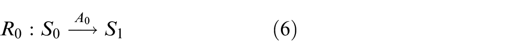
Markov Decision Process (MDP) is a mathematical model for sequential decision making, which is used to simulate the achievable policies and rewards of agent systems in the environment where the system state has the Markov property.

As shown in the equation (5), the mathematical description of the property of MDP is that the future is only related to the current state and has nothing to do with the past.

$$P\left(S_{k+1}|S_k\right)=P(S_{k+1}|S_k,S_{k-1},\cdots ,S_1)$$

(5)

This is consistent with the adjustment strategy in the formation of UAVs, that is, what needs to be considered in the formation adjustment process is not the global adjustment scheme of the whole process and the whole state. It only needs to calculate the adjustment direction of the next UAV according to the current UAV transmitting signal and the UAV receiving signal, without paying attention to the previous adjustment process, according to the current formation signal receiving and sending state. The next adjustment scheme can be determined according to the current formation signal receiving state. The adjustment strategy MDP model can be constructed as shown below:

In Figure 4, $A_k$ is the adjustment policy; $S_k$ is the current state of the UAV formation, and can reach the next new state $S_{k+1}$ after adjustment. $R_k$ is the reward and punishment function, which obtained by the UAV formation when it transfers from the current state to the next state. 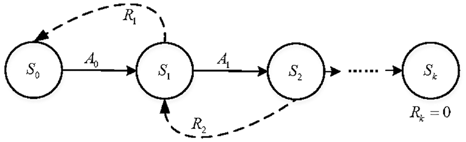In this paper, the reward and punishment function of an individual UAV is defined as the Angle difference value between the UAV and the standard node.

Figure 4.

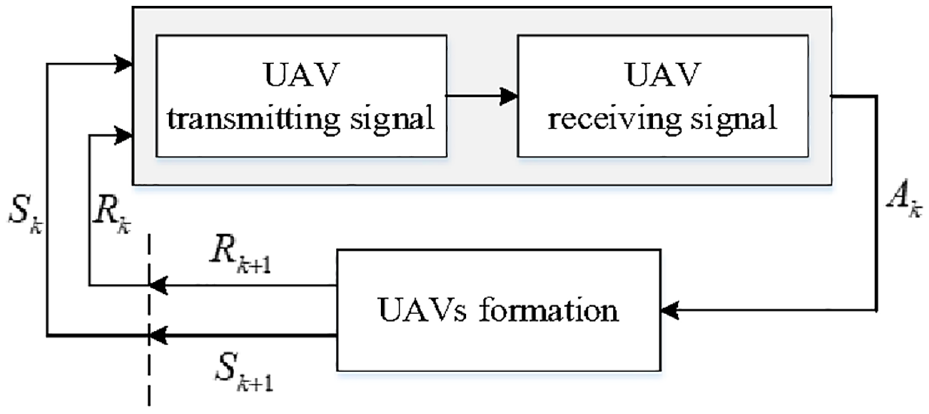
Adjustment policy MDP model.

In the initial stage, the UAV formation has an initial state $S_0$ . At this time, the UAV formation does not undergo any strategy adjustment, but there is a certain deviation between the position of UAV in the formation and the position in standard formation. When a UAV receives the angle signal sent by the other UAVs that send signals, it finds that it has a deviation. The adjustment strategy $A_0$ is calculated by the algorithm to adjust its position, leave the formation state $S_0$ , enter the state $S_1$ , and obtain the reward and punishment value $R_1$ generated in the process, which can be expressed as:

$$R_0:S_0\stackrel{A_0}{\to }{S}_1$$

(6)

Throughout the entire process of adjusting the UAV formation strategy, the MDP model is consistently applied in an iterative fashion. This application continues in a cyclical manner until the UAV formation aligns perfectly with the standard formation, as depicted in Figure 5. It is crucial to highlight that the reward and punishment function, which is integral to the MDP model, is specifically designed to measure the discrepancy between the UAVs’ current state and the ideal, standard formation state. Consequently, the ultimate objective of the MDP model’s adjustment strategy is to attain a formation state where this reward and punishment function evaluates to zero, indicating that the UAV formation has been successfully corrected with no remaining deviation. This target state signifies the achievement of optimal formation configuration, free from any discrepancies. The utilization of the MDP model is particularly beneficial in scenarios that demand precise and efficient decision-making, such as coordinating the movements of a UAV swarm. It allows for the strategic planning of each UAV’s maneuvers based on the current state and the defined reward structure, thereby ensuring the most effective path to the desired formation is taken. It should be noted that since the reward and punishment function $R$ is defined as the deviation between the current state and the standard formation state, so, the destination of MDPmodel adjustment strategy is formation state $S_k$ , which the value of reward and punishment function $R_k$ is zero.

Figure 5.

Adjustment strategy process using MDP model.

Establishment and solution of azimuth-only passive positioning model in conical formation

Establishment of azimuth-only passive positioning model in conical formation

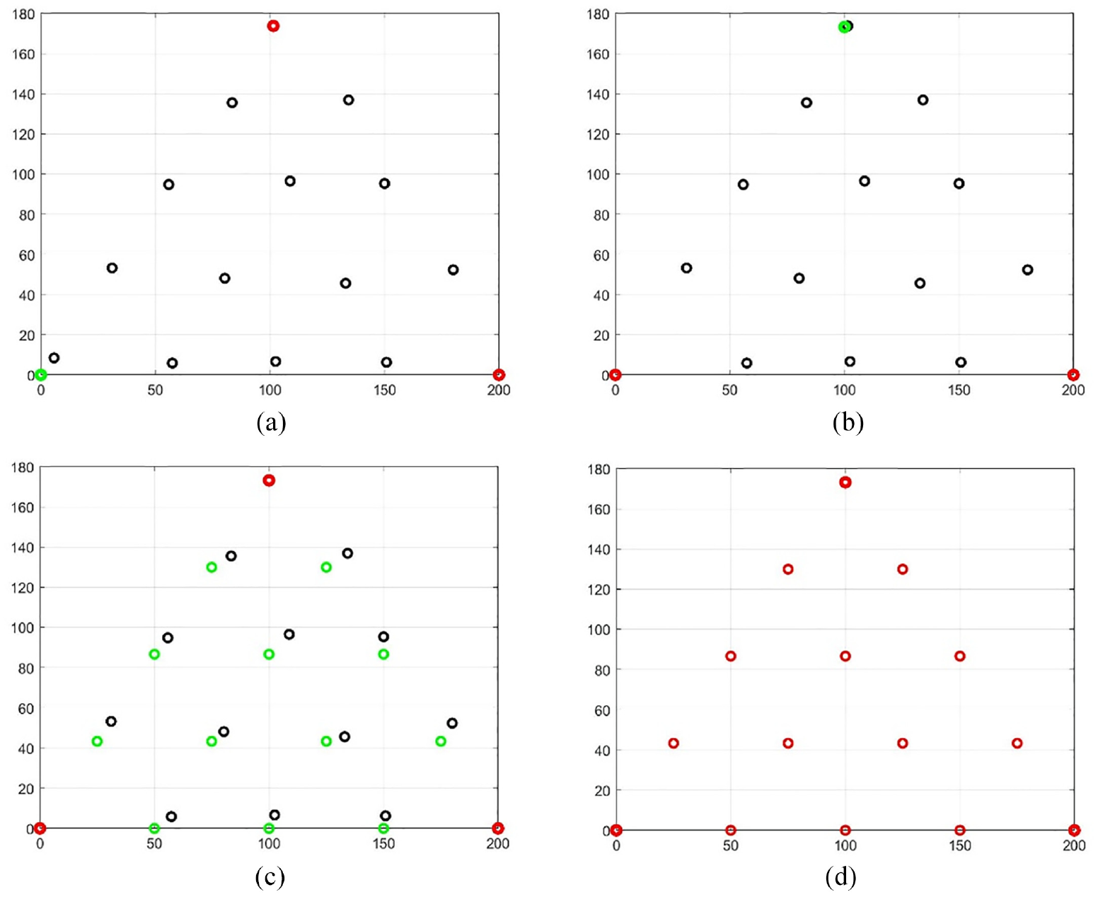
In order to ensure the minimum probability of UAV detection in the electromagnetic silence environment, it is necessary to select as few as possible the number of UAVs transmitting signals. However, in the angle positioning, at least 3 UAVs are needed for azimuth passive positioning. Assuming that UAVs is in a conical formation. Each time, the vertex UAV (UAV numbered 1) in the conical formation and any one or two UAVs located on the edge of the triangle are selected to establish the model (Figure 6).

Figure 6.

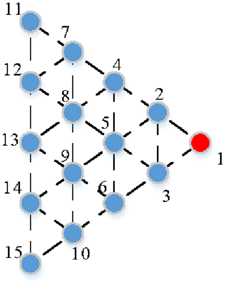
UAV formation.

Since the spacing between individual UAVs and neighboring UAVs is known to be 50 km, the overall situation of the formation of UAVs is unknown, and there are UAVs with deviated positions, which need to be located passively by bearing. Therefore, it is necessary to determine the overall frame of the conical formation, that is, the position of the vertex, in the initial stage. The directed graph model for the formation nodes can be constructed as follows:

$$G_{1,11}^{15}:〈{\stackrel{⌣}{u}}_{15},{\stackrel{⌢}{u}}_1,{\stackrel{⌢}{u}}_{11}〉\to {\alpha }_{1,11}^{15}$$

(7)

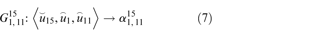
Although the phase angle force model can obtain the adjustment direction of the UAV, it also needs to solve the adjustment size accurately to obtain the accurate adjustment vector of the UAV. Figure 7 shows the diagram of UAV adjustment vector, the UAV No.1 and No.11 transmitting signals to the UAV No.15 which is at the standard nodes. At this time, the known parameters can be directly obtained as follows: the angle $\beta$ of the standard conical formation, the vector between the cone vertices $C$ , $d$ , and $f$ . The position of UAV No.15’ is the position of UAV with slightly disturbed, at this time, it can obtain the angle $\alpha$ corresponding to the two UAVs transmitting signals. On this basis, it is necessary to solve the adjustment vector $e$ of the perturbed position of UAV No.15’ to adjust to the standard position of UAV No.15.

Figure 7.

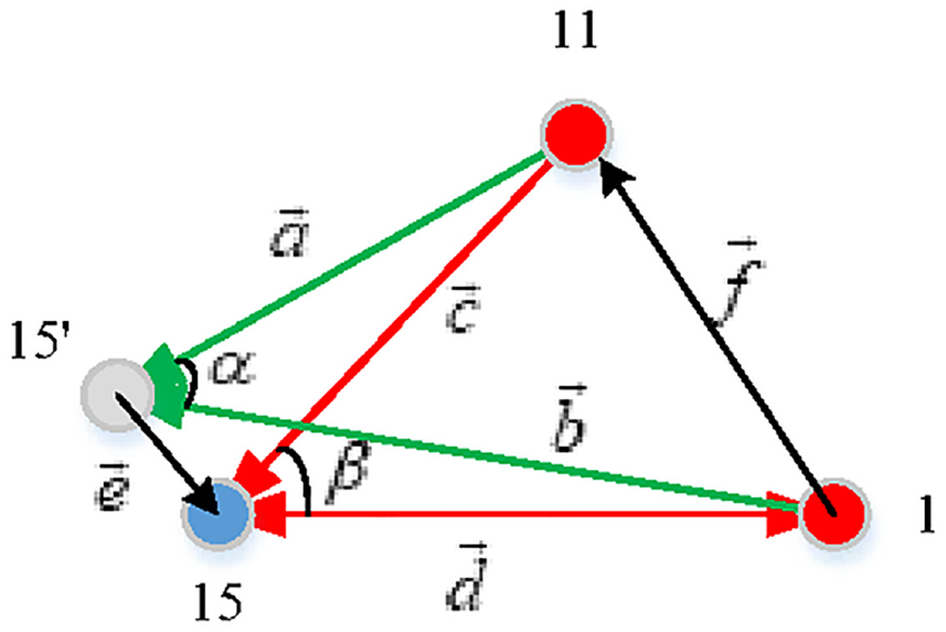
Diagram of adjustment vector of UAV.

According to the relationship between the law of cosines and the triangle vector, it can be concluded that:

$$\cos \left(\alpha \right)=\frac{\overrightarrow{a}·\overrightarrow{b}}{\left|\overrightarrow{a}\right|\left|\overrightarrow{b}\right|}$$

(8)

$$\cos \left(\beta \right)=\frac{\overrightarrow{c}·\overrightarrow{d}}{\left|\overrightarrow{c}\right|\left|\overrightarrow{d}\right|}\beta =60°$$

(9)

From the relationship between the vectors, it is easy to obtain:

$$\{\begin{array}{c}\overrightarrow{e}=\overrightarrow{c}-\overrightarrow{a}\hfill \\ \multicolumn{1}{c}{\overrightarrow{e}=\overrightarrow{d}-\overrightarrow{b}}\\ \multicolumn{1}{c}{\overrightarrow{f}=\overrightarrow{d}-\overrightarrow{c}}\\ \multicolumn{1}{c}{\overrightarrow{f}=\overrightarrow{b}-\overrightarrow{a}}\end{array}$$

(10)

In a standard formation, the resulting conical formation is an equilateral triangle, so its three sides have exactly the same length:

$$\Vert \overrightarrow{c}\Vert =\Vert \overrightarrow{d}\Vert =\Vert \overrightarrow{f}\Vert =200$$

(11)

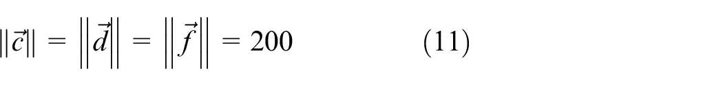
According to the formula (8)–(11), it can be seen that its unknown quantities are, $a$ , $b$ , and $e$ , and there are eight formulas, which can solve the adjustment strategy of a single UAV as:

$$R_1^{15}:S_0^{15}\stackrel{A_{15}=\overrightarrow{e}}{\to }{S}_1^{15}$$

(12)

Where: $A_{15}=\overrightarrow{e}$ is the adjustment strategy vector of the UAV No.15 adjusted from the actual position to the standard node position; $R_1^{15}$ is the reward value before and after adjustment and $S_1^{15}=\Vert \overrightarrow{e}\Vert$ .

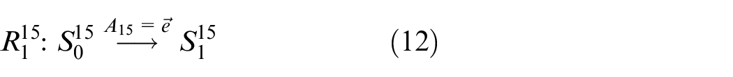
Similarly, in the second state transition step of the MDP model, the standard position of another cone vertex of UAV No.11 can be obtained by using UAV No.1 and UAV No.15 whose position has been determined as the UAV sending signal:

$$R_2^{11}:S_1^{11}\stackrel{A_{11}}{\to }{S}_2^{11}$$

(13)

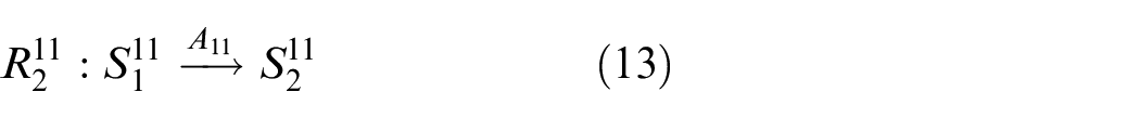
After two steps of state transfer, the accurate positions of the three vertices of the UAV in the cone formation can be determined. Because the UAV No.1 is the benchmark node, all the UAVs are adjusted in formation relative to the UAV No.1.

Then, the vertices of the three cone formations are used as the UAVs transmitting signals. Assuming that the standard node position of any UAV $k\prime$ inside the cone is $k$ .

In Figure 8, the known parameters are the angle formed by the UAV receiving the signal to the corresponding UAV transmitting the signal: ${\alpha }_1$ , ${\alpha }_2$ , ${\alpha }_3$ , ${\beta }_1$ , ${\beta }_2$ , and ${\beta }_3$ , and the standard point UAV and the UAV transmitting the signal form vectors. For ease of understanding, all vectors are represented by two-dimensional coordinates, as shown in the Figure 8. The vector between any two UAV nodes $m$ , $n$ is defined as follows:

$${\overrightarrow{e}}_m^n=(x_n-x_m,y_n-y_m)$$

(14)

that is, the vector ${\overrightarrow{e}}_m^n$ , denotes the pointing vector from node $m$ to node $n$ .

Figure 8.

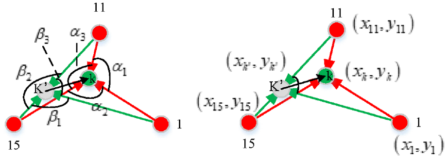
Illustration of the UAV adjustment strategy.

It is easy to know that in Figure 8, the known UAV node vectors are: ${\overrightarrow{e}}_1^{15}$ , ${\overrightarrow{e}}_1^{11}$ , ${\overrightarrow{e}}_{11}^{15}$ , ${\overrightarrow{e}}_1^k$ , ${\overrightarrow{e}}_{11}^k$ , and ${\overrightarrow{e}}_{15}^k$ , and the azimuth-only passive localization problem in the conical formation can be transformed into calculating the relative vector ${\overrightarrow{e}}_{k\prime }^k$ from the actual UAV position $k\prime$ to the standard node position $k$ .

From the angle information, the formula relationship between angle and UAV node vector can be obtained as shown in equations (15) and (16).

$$\{\begin{array}{c}\cos \left({\alpha }_1\right)=\frac{{\overrightarrow{e}}_k^1·{\overrightarrow{e}}_k^{11}}{\left|{\overrightarrow{e}}_k^1\right|\left|{\overrightarrow{e}}_k^{11}\right|}\hfill \\ \cos \left({\alpha }_2\right)=\frac{{\overrightarrow{e}}_k^1·{\overrightarrow{e}}_k^{15}}{\left|{\overrightarrow{e}}_k^1\right|\left|{\overrightarrow{e}}_k^{15}\right|}\hfill \\ \cos \left({\alpha }_3\right)=\frac{{\overrightarrow{e}}_k^{15}·{\overrightarrow{e}}_k^{11}}{\left|{\overrightarrow{e}}_k^{15}\right|\left|{\overrightarrow{e}}_k^{11}\right|}\hfill \end{array}$$

(15)

$$\{\begin{array}{c}\cos \left({\beta }_1\right)=\frac{{\overrightarrow{e}}_{k\prime }^1·{\overrightarrow{e}}_{k\prime }^{11}}{\left|{\overrightarrow{e}}_{k\prime }^1\right|\left|{\overrightarrow{e}}_{k\prime }^{11}\right|}\hfill \\ \cos \left({\beta }_2\right)=\frac{{\overrightarrow{e}}_{k\prime }^1·{\overrightarrow{e}}_{k\prime }^{15}}{\left|{\overrightarrow{e}}_{k\prime }^1\right|\left|{\overrightarrow{e}}_{k\prime }^{15}\right|}\hfill \\ \cos \left({\beta }_3\right)=\frac{{\overrightarrow{e}}_{k\prime }^{15}·{\overrightarrow{e}}_{k\prime }^{11}}{\left|{\overrightarrow{e}}_{k\prime }^{15}\right|\left|{\overrightarrow{e}}_{k\prime }^{11}\right|}\hfill \end{array}$$

(16)

According to the superposition relationship between the angles, the sum of the internal angles of the triangle is 180°, and the sum of the circumferential angles of a point relative to the other three distributed points is 360°, which can be obtained as follows:

$$\{\begin{array}{c}\cos ({\beta }_1+{\beta }_2)=\cos \left({\beta }_3\right)\hfill \\ \multicolumn{1}{c}{\cos ({\beta }_2+{\beta }_3)=\cos \left({\beta }_1\right)}\\ \multicolumn{1}{c}{\cos ({\beta }_1+{\beta }_3)=\cos \left({\beta }_2\right)}\end{array}$$

(17)

And then according to the relationship between the vectors, the vector equation can be expressed by the angle relationship relate to ${\overrightarrow{e}}_{k\prime }^k$ .

Solution of bearing-only passive localization model in conical suicid-formation

In the initial stage, due to the small number of parameter variables, the complex variable equations can be solved by using the solve function in MATLAB 12.0a version, and the parameters to be solved are set as follows: adjusting the vertex UAV ${\overrightarrow{e}}_{11\prime }^{11}$ of the conical formation during the first state transition in the formation strategy.

When the UAV ${\overrightarrow{e}}_{15\prime }^{15}$ at the vertex node of the cone formation in the second state transition of the adjusted formation strategy needs to be solved, any offset UAV ${\overrightarrow{e}}_{k\prime }^k$ inside the cone in the third state transition of the adjusted formation strategy needs to be solved. Due to the large number of variable parameters, the formula expression between the independent variables and the results cannot be directly obtained. At this time, the Runge-Kutta method is set to solve the approximate optimal result^27,28 and the minimum step size is 0.1. The solution result of ${\overrightarrow{e}}_{15\prime }^{15}$ and ${\overrightarrow{e}}_{k\prime }^k$ can be obtained.

Simulation experiment and analysis

Setting of initial environment

A standard cone-shaped formation was constructed in MATLAB, a total of 15 UAVs were arranged according to the standard node, and the distance between each aircraft and its neighbors was 50 km. On this basis, a disturbance value of 0–10 km was applied to all UAVs to make them deviate from the position of standard formation node. The arrangement of the initial environment is shown in Figure 9, and the node coordinates are shown in Table 1.

Figure 9.

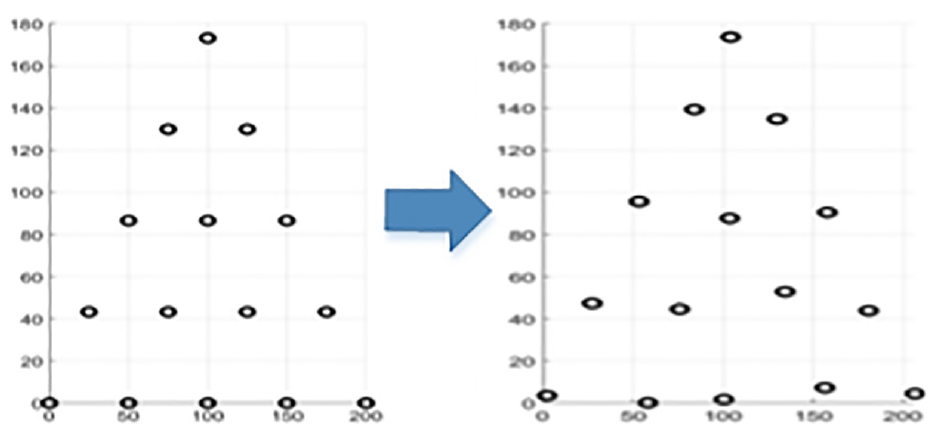
Initial standard environment versus perturbed environment.

Table 1.

UAV position coordinates of the initial standard environment and the disturbed environment.

Standard cone formation
X-coordinate	Y-coordinate
104.17	173.70
84.03	139.35
129.91	134.80
53.38	95.60
103.69	87.71
157.80	90.50
27.42	47.34
75.96	44.62
134.42	52.86
180.75	43.90
2.35	3.53
58.21	0.15
100.43	1.69
156.49	7.32
206.48	4.51
Disturbance cone formation
X-coordinate	Y-coordinate
100.00	173.21
75.00	129.90
125.00	129.90
50.00	86.60
100.00	86.60
150.00	86.60
25.00	43.30
75.00	43.30
125.00	43.30
175.00	43.30
0.00	0.00
50.00	0.00
100.00	0.00
150.00	0.00
200.00	0.00

Simulation experiment and analysis

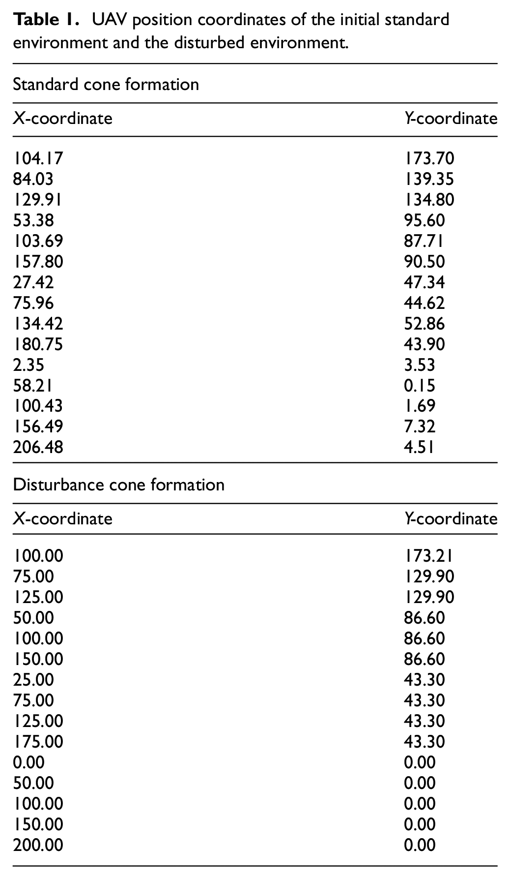
Based on the above initial environment settings and the constructed model, the simulation experiment is carried out in MATLAB as shown below. Where red points are the UAVs that transit the signal, green points are the UAVs that receive the signal, and black points are the actual position of the UAVs. It can be seen that after three MDPS, all the UAVs with offset positions can reach the standard nodes in the cone formation.

For the convenience of exposition, the simulation result diagram of Figure 10 is transformed into the process diagram shown in Figure 11. FIG. In the formation state 1, since the exact positions of all the UAVs in the formation are not known, vertex UAV No.1 is selected as the relative coordinate node, and then another vertex node is selected (note that the position of this vertex node is also inaccurate), so as to adjust the vertex UAV receiving signals sent by the two vertex node UAVs to the standard node position. Similarly, in the next step, Due to the existence of two standard node UAVs, the last vertex UAV can be adjusted to reach the standard position.

Figure 10.

Simulation experiment of UAV formation based on MATLAB: (a) formation adjustment – State 1, (b) formation adjustment – State 2, (c) formation adjustment – State 3, and (d) final standard conical formation.

Figure 11.

Schematic diagram of UAV formation simulation experiment: (a) formation – State 1, (b) formation – State 2, (c) formation – State 3, and (d) standard conical formation.

After having the accurate relative positions of the three vertex node UAVs in the conical formation, the three UAVs were allowed to broadcast their azimuth information at the same time. According to the relative positions and the passive localization model constructed, all UAVs adjusted their positions at the same time, and finally formed a standard formation.

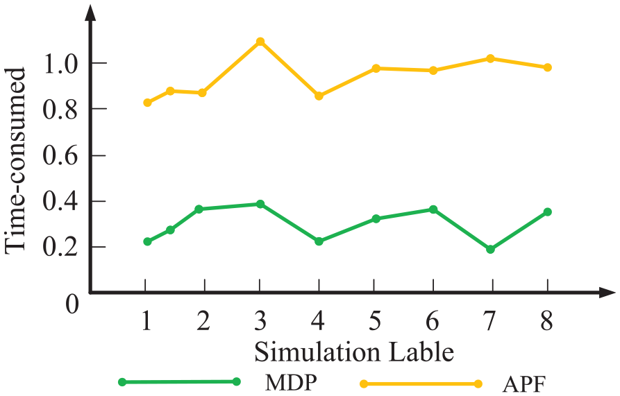
The comparative simulation experiment is depicted in Figure 12, where the green line represents the MDP method constructed in this paper, and the yellow line signifies the Artificial Potential Field(APF) method. It can be observed that under identical task conditions, the MDP method developed in this study facilitates rapid information transfer among the UAV swarm, resulting in shorter time consumption and ensuring the safety of the UAV swarm’s flight. In contrast, the APF method, which necessitates the perception and construction of global potential field information and involves complex decision-making, does not perform as well in a multi-UAV swarm. It often requires a longer time to complete the same task due to the complexity of the global field information it must process and the decisions it must make in a dynamic and multi-agent environment.

Figure 12.

Comparing simulation experiment.

The MDP method’s advantage lies in its ability to model decision-making problems in situations involving uncertainty and to optimize the decision-making process over time. This is particularly beneficial for UAV swarms where quick and efficient decisions are paramount for coordinated and safe operations. On the other hand, the APF method, while effective in certain scenarios, may struggle with scalability and efficiency when applied to larger swarms or more complex tasks. The comparative results highlight the importance of selecting an appropriate algorithm for the specific requirements and constraints of the UAV swarm operation, with the MDP method showing promise for scenarios demanding swift and reliable decision-making processes.

Summary

In this paper, the adjustment model of individual UAV, the directed graph model of formation node, and the MDP model of adjustment strategy are constructed. Based on the relevant factor model, the idea of mutual force is proposed. Through the description of Markov decision process, the azimuth-only passive localization model in conical suicidal-formation is established, and it is solved in MATLAB. Although it can solve the problem of UAV passive formation in electromagnetic silence environment, it still has the following shortcomings. First, the algorithm is not extended to the three-dimensional environment, and the algorithm is only described and simulated in the two-dimensional plane. The other is that the algorithm has not been tested in the actual environment and has not been tested by practical practice. In the later stage, it will continue to conduct in-depth research.