
Abstract
State estimation is a fundamental necessity for any application involving autonomous robots. This paper describes a visual-aided inertial navigation and mapping system for application to autonomous robots. The system, which relies on Kalman filtering, is designed to fuse the measurements obtained from a monocular camera, an inertial measurement unit (IMU) and a position sensor (GPS). The estimated state consists of the full state of the vehicle: the position, orientation, their first derivatives and the parameter errors of the inertial sensors (i.e., the bias of gyroscopes and accelerometers). The system also provides the spatial locations of the visual features observed by the camera. The proposed scheme was designed by considering the limited resources commonly available in small mobile robots, while it is intended to be applied to cluttered environments in order to perform fully vision-based navigation in periods where the position sensor is not available. Moreover, the estimated map of visual features would be suitable for multiple tasks: i) terrain analysis; ii) three-dimensional (3D) scene reconstruction; iii) localization, detection or perception of obstacles and generating trajectories to navigate around these obstacles; and iv) autonomous exploration. In this work, simulations and experiments with real data are presented in order to validate and demonstrate the performance of the proposal.
1. Introduction
In recent years, many researchers have addressed the issue of making vehicles more and more autonomous. In this context, the state estimation of the six degrees of freedom (DOFs) of the vehicle (i.e., its attitude and position) is a fundamental necessity for any application involving autonomy.
Even though, this problem is seemingly solved for open outdoor domains by an on-board Global Positioning System (GPS) unit and inertial measurements units (IMU), as well an integrated version: an inertial navigation system (INS). Contrary, unknown, cluttered and GPS-denied environments still pose a considerable challenge. While attitude estimation is well handled by available systems, GPS-based position estimation can have some drawbacks. GPS is not a reliable service as its availability can be limited by urban canyons and it is completely unavailable in indoor environments. The aforementioned issues have prompted recent studies to move towards the use of cameras for performing visual-based navigation in periods or circumstances where the position sensor (i.e., GPS) is not available. Cameras are well adapted for embedded systems: they are light, cheap and power-saving.
1.1. Related work
Several strategies related to visual-based navigation can be found in the literature. Some systems that use vision for navigation require previous knowledge of the whole environment. In this case, some kind of guided or automated pretraining is needed in order to learn visual patterns in the environment, which are recognized and used later as visual clues at the navigation stage. Examples of guided pretraining methods are [1] and [2]. In [3, 4], during the navigation, the position is determined matching the online image with previously recorded images. Usually, the application of this kind of method is limited to environments where the training phase takes place.
Another kind of system has been designed to perceive the environment as it is navigated through. Behaviour-based navigation systems can rely on qualitative image information (examples are [5, 6] and [7]). In this kind of system, it is avoided as much as possible using, computing or generating accurate numerical data, such as distances, position coordinates, velocity, projections from the image plane onto the real world plane, or contact time to the obstacles. Due to its critical dependence on unprocessed sensorial data, this kind of method is highly dependent on the change in the imaging conditions.
Approaches, such as [8] or [9], rely on optical flow information, as do [10] and [11], although the optical flow is combined with stereo information in their case. A related approach to the optical flow scheme is the tracking of visual features. In this case, however, instead of estimating the visual flow of the whole image (i.e., every pixel), a set of strong visual features, such as corners, lines and objects outlines, are detected and tracked over time for as much as it may be possible. Examples of methods based on the former approach are [12] and [13], in which the computation of the camera motion is obtained from a homography. In [14], inertial data obtained from an IMU is combined with visual tracking information.
Some systems can build a map of the environment while exploring it. The maps can have a topological representation, as in [15] and [16], or a metric representation. Occupancy grid-based strategies represent one of the early approaches to representing metric maps; some examples are [17] and [18] However, occupancy grid-based strategies can be computationally inefficient for path planning and localization, especially in complex and great indoor environments.
Another family of approaches relies on simultaneous localization and mapping (SLAM) strategies. In this case, the system must operate in an a priori unknown environment using only on-board sensors to simultaneously build a map of its surroundings and localize itself [19]. Usually, this kind of system also relies on the tracking of a set of prominent visual features. As these visual features typically have a spatial meaning, the information obtained from the visual measurements can be used to replace range sensors: the lasers are often expensive and heavy, while the operation range of ultrasonics is limited. In this sense, the appearance and spatial information provided by cameras can be useful for multiple tasks, such as: i) terrain analysis; ii) 3D scene reconstruction; iii) localization, detection or perception of obstacles and generating trajectories to navigate around these obstacles; and for iv) autonomous exploration.
Currently, there are two main approaches to implementing vision-based SLAM systems: i) filtering-based methods (see [20–22] and [23]), and ii) optimization-based methods (see [24] and [25]). While the former approach is shown to give accurate results when the availability of computational power is enough, filtering-based SLAM methods might still be beneficial if limited processing power is available [26]. While the benefit obtained from constructing a map of the robot's environment is self-evident, it comes together with a considerable increase in computational requirements. The former issue is due to the fact that, in visual SLAM, the visual features are included in the state vector. When the number of map features in the system state increases, computational cost grows rapidly, such that it consequently becomes difficult to maintain real-time performance. The above becomes more evident when limited hardware is available. On the other hand, in a context of visual odometry, this problem can be partially mitigated by removing old features from the state in order to stabilize the computational cost per frame [27].
In applications involving mobile robots, it is very common to have a set of sensors available for use. Incorporating complementary or redundant data from multiple sensors can improve the robustness and accuracy of the system. In this sense, sensor fusion that uses, for instance, IMU, GPS and cameras is not novel. Some examples of multi-sensor navigation algorithms are [28–31] and [32].
1.2. Objective
This work presents a novel method for implementing a visual odometry and mapping system. The method is mainly intended to be applied to autonomous mobile robots with limited computational resources. The proposed scheme is related, on the one hand, to visual odometry methods, which make use of the optical flow obtained from prominent visual features in order to compute the camera movement. On the other hand, it is related to visual SLAM methods in the sense that a map of the environment is built and used for refining the estimations. Some contributions and differences from previous work are:
In contrast with visual SLAM approaches, the system state in the proposed scheme is never augmented with the state of map features. Instead, each map feature is managed independently from the state of the vehicle, as well as from other map features. The above technique, which perhaps represents the main contribution of this work, allows a reduction in the computational requirements.
A novel technique based on two-step architecture is proposed in order to initialize and measure the visual features in a robust and efficient manner. The proposed scheme makes use of the information obtained from monocular measurements and allows advantage to be taken of the information provided by visual features, whose depth estimation is not well conditioned.
The use of an extended Kalman filter (EKF) in direct configuration allows a straightforward integration with additional sensors, such as inertial sensors (i.e., gyroscopes and accelerometers), and GPS, when it is available.
It is important to note that the proposed system should not be considered as a true SLAM system; rather, and just in case, it should be considered as an approximation of it. This is because the cross-correlation information of the feature uncertainty, which is contained in the system covariance matrix, is discarded on behalf of computational cost reduction. Fortunately, the experimental results would suggest that the proposed scheme is useful when applied to a context of visual-based navigation.
1.3. Paper outline
The paper is organized as follows. Section 2 presents the system parameterization and assumptions. Section 3 describes the proposed system in detail. In Section 4, experimental results, carried out using simulations and real data, are presented in order to validate and demonstrate the performance of the proposal. Finally, Section 5 presents conclusions and final remarks.
2. System Parametrization and Assumptions
The main goal of the proposed method is to estimate the following system state x:

where
The proposed method is intended for local autonomous vehicle navigation. In this case, the local tangent frame is used as the navigation reference frame and, in turn, the initial position of the vehicle defines its origin. The navigation coordinate frame follows the NED (north-east-down) convention. In this work, the magnitudes expressed in the i) navigation frame, ii) vehicle (robot) frame and iii) camera frame are respectively denoted by the superscripts
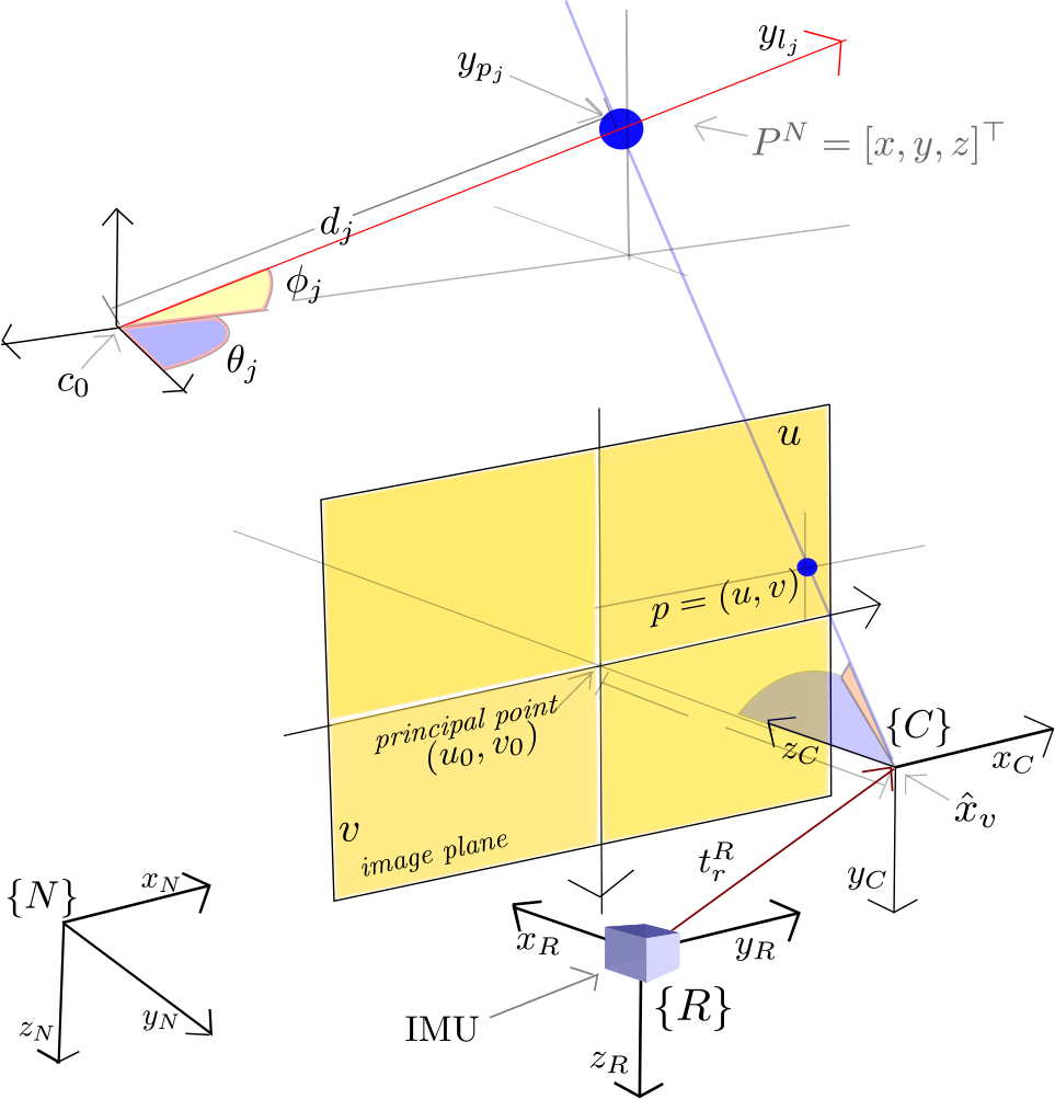
System parametrization. The local tangent frame is used as the navigation reference frame N . Furthermore, it is assumed that the coordinate frame of the IMU is aligned with the origin of the coordinate frame of the robot R .
The position and orientation of the camera, in respect of the vehicle coordinate frame
For estimating the system state x, the following kinds of sensorial measurement are considered:
2.1. Visual measurements
A standard monocular camera is considered (see Figure 1). In this case, the availability, at each k frame, of a list of

where
A central projection camera model is assumed. In this case, the image plane is located in front of the camera's origin, upon which a non-inverted image is formed (Figure 1.) The camera frame
The

where u and v are the coordinates of the image point p expressed in pixels units and:

being
Inversely, a directional vector

The vector
The distortion caused by the camera lens is considered in relation to the model described in [34]. Using the former model (and its inverse form), undistorted pixel coordinates
2.2. Inertial measurements
The angular rate

where
The acceleration of the vehicle
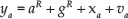
where
2.3. GPS measurements
Position and course measurements (yr and yθ, respectively) are obtained from the GPS, whenever possible, and are modelled by:

where vr is a Gaussian white noise with PSD
3. Method Description
The architecture of the system is defined by the typical loop of prediction-update steps in the EKF in direct configuration, in which the EKF propagates the vehicle state. Whenever possible, the filter is updated by the filter update equations, in which visual information is obtained from the monocular camera as well as the data obtained from the additional sensors. The estimation of the features’ map location is carried out, in an independent manner, by the main EKF process.
3.1. System initialization
An initial period of time is used for system initialization tasks. During this period, the vehicle is assumed to be non-accelerating. The initial system state
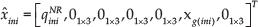
where
3.2. System prediction
At every step k, when gyroscope and accelerometer measurements are available, the predicted system state

where

The state covariance matrix P is taken a step forward by:

The Jacobian
The measurement noise of the gyroscopes and accelerometers (respectively, vg and va) are incorporated into the system by means of the process noise covariance matrix U through parameters

3.3. Attitude and position updates
In order to correct and limit drift in the estimated system state
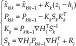
where zi is the current measurement and
Each filter update is carried out using equation 14, along with zi, hi,
3.3.1. Roll and pitch measurement model
If the vehicle is not accelerating (i.e.,
The gravity vector g is predicted to be measured by the accelerometers as hg:

where gc is the gravity constant and
3.3.2. Position and heading measurement model
In this work, a loosely coupled approach is used for incorporating data provided by the GPS unit, whenever it is possible. In a loosely coupled approach, the high level outputs provided by the GPS unit are directly incorporated into the system state through their corresponding measurement prediction model.
The model hr, which is used for predicting GPS measurements about the vehicle position, is simply:

The course (heading) of the vehicle is predicted by the following measurement model hγ:

where
3.3.3. Dynamical constraints
Prior knowledge about the vehicle dynamics can be incorporated into the system through filter updates. For instance, in the case of a car-like vehicle, nonholonomic constraints are incorporated in the form of zero velocity updates. For this purpose, it can be assumed that the velocity of the vehicle, in its own reference frame, should be measured as

where
3.4. Visual aid
3.4.1. Initialization of visual features
At the first instant k, when a new visual feature

where

where
3.4.2. Applying epipolar constraints
Depth information cannot be obtained in a single measurement when bearing sensors (i.e., monocular camera) are used. To infer the depth of a feature, the sensor must observe it repeatedly as it moves through its environment, estimating the angle from the feature to the sensor centre. The difference between those angle measurements is the parallax, which is the key that allows estimating feature depth. Nevertheless, features with unknown depth or with huge uncertainty in depth can still provide useful information, such as for very far away landmarks, which will never produce a parallax, but can improve camera pose estimates. The following technique, which is based on epipolar constraints, is used for incorporating information from visual features with unknown or ill-conditioned depth. Epipolar constraints have been successfully used in the past for improving estimates in visual-based navigation systems (e.g., [37]). In this work, a version of the constraint is derived by considering the particularities of the proposed system.
If the camera moves from the location at which a feature is initialized, then this feature, which is first modelled as a 3D semi-line

Model measurement for visual features with ill-conditioned depth
The epipole er is computed by projecting

where
Assuming that, for the current frame, n visual measurements are available for features with ill-conditioned depth, the filter is updated as follows:
3.4.3. Estimating feature depth
For minimizing computational cost, and unlike typical filtered-based SLAM methods, where the vector state is augmented in order to incorporate the map features, the map in the proposed method is maintained in an independent manner of the state of the vehicle; hence, the state of the features cannot be updated directly through the filter update equations when new measurements are available. Instead, when a new measurement
First, a hypothesis of depth dj is computed by:

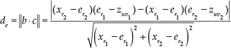
where
where β is the angle defined by h1 and el. h1 is the normalized directional vector
γ is the angle defined by h2 and
3.4.4. 3D map management
As previously stated before, the parallax produced by sensor movements permits the estimation of the depth of the features. In the case of an indoor sequence, a displacement of centimetres is enough to produce a parallax; on the other hand, the more distant the feature, the more the sensor has to travel to produce a parallax.
In [38], it is shown that only a few degrees of parallax are enough to reduce the uncertainty related to depth estimation. Then, when the parallax of a j feature is greater than a threshold (
First, the Euclidean representation
Assuming that, for the current frame, n visual measurements are available for 3D features, the filter is updated as follows:
4. Experimental Results
Experiments, using both synthetic data obtained by simulations and real data, were performed in order to validate the performance of the proposed method. A MATLAB implementation was used for this purpose.
4.1. Experiments with simulations
In experiments, a mobile robot was simulated moving through environments composed by 3D points, which can be used by the system as visual landmarks. The simulated vehicle is equipped with: i) inertial sensors, ii) a position sensor, and iii) a monocular camera. The position sensor is used only at the beginning of the trajectory for recovering the metric scale of the environment, after which it is turned off for the purpose of validating the performance of the method in which visual-based navigation is used.
The following parameters values were used in simulations: i) for emulating inertial sensors,
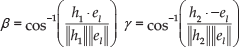
A Monte Carlo simulation was carried out in order to validate the improvement obtained when visual information is incorporated into the system through the proposed scheme. The upper and middle plots give an example of the trajectories obtained with and without visual information. The lower plot shows the average mean absolute error (MAE) in the position obtained after 20 runs. The experimental results clearly show that position's drift is considerable lower when the system makes use of the visual information.
4.1.1. Visual aiding vs. no visual aiding
Figure 3 (upper plot) shows the simulated 3D environment, which was used to perform this experiment. In this case, the land vehicle was moved in order to follow a spiral-like trajectory (see middle plot). The area, in which the vehicle is moving, is surrounded by a wall of landmarks that can be used by the system as visual features. As expected, the drift in estimations is considerable lower when visual information is incorporated into the system. Figure 3 (lower plot) shows the average MAE in the position obtained after 20 Monte Carlo runs of the simulation.
4.1.2. Proposed method vs. standard EKF-SLAM
Figure 4 shows two of the simulated environments used in this experiment. In the first series of experiments (a), the robot was moved in order to follow a spiral-like trajectory. The area, where the vehicle is moving is surrounded by a wall of landmarks. In these experiments, the camera was fixed, pointing toward to the axis of movement of the robot. In the second series of experiments (b), the robot was moved, following a wave-like trajectory. The environment, where the vehicle is moving, is composed by clouds of landmarks located in random positions. In these experiments, the camera was fixed, pointing perpendicular to the axis of movement of the robot.

In simulations, a land vehicle was moved through different environments, which were composed by 3D points, emulating potential visual landmarks. The position sensors were only used at the beginning of the trajectory. The rest of the trajectory was performed under visual navigation conditions.

MAE: Proposed method vs. system state augmentation. Experiment (a) - left plot. Experiment (b) - right plot.
In order to gain more insight about the performance of the proposed scheme, a variant of the proposal was also implemented, in this case by using system state augmentation (standard EKF-SLAM methodology). Figure 5 shows the average MAE in the position obtained after 20 Monte Carlo runs of the simulation, using the proposed method and system state augmentation. It can be observed that the progression of the MAE over time, which was obtained in scenarios (a) and (b), is very similar. On the other hand, Table 1 clearly shows the benefits obtained with the proposed method in terms of computational cost. In this case, the performance of the variant, which uses system state augmentation, quickly degrades as the number of visual features being tracked increases. In experiments (a), where the average number of visual features being tracked per frame is low, the execution time of the variant is slightly higher than the proposed method. However, in experiments (b), where the average number of features being tracked is higher, the execution time of the variant is almost three times the execution time of the proposed method.
Execution time obtained using the proposed method and system augmentation. The third column indicates the average number of visual features being tracked per frame.

4.2. Experiments with real data
In order to test the performance of the proposed method with real data, the MATLAB implementation was executed offline using the Malaga data set [39] as input signals. This data set is freely available online and contains several sources of sensor signals along with accurate ground truth. In the experiments, the following signals were used: i) inertial (accelerometer and gyroscope) measurements, available at 100; ii) GPS measurements, available at 1; iii) visual information, obtained from a frontal camera at seven frames per second (fps), and with a resolution of 512×384 pixels. The sensors were mounted over an electric buggy-type vehicle, (see [39] for a complete description). The experiments presented here correspond to a vehicle moving across a car park.

Aerial view of the estimated map and trajectory, using real data from sensors mounted in an electric buggy-type vehicle, which is moving in a car park. The GPS signal (blue) was only used at the beginning of the trajectory for recovering the metric scale. The visual-based estimated trajectory is indicated in red.
In the same manner as the simulations, the proposed method was compared against the standard EKF-SLAM methodology (system augmentation), except that real data were used in this case. Figure 6 shows the map and trajectory obtained by the proposed method for a route with a duration of 110. Note that GPS was only used at the beginning of the trajectory for recovering the metric scale of the world. Table 2 shows the experimental results obtained with both the proposed method and the standard EKF-SLAM methodology.
Experimental results with real data

The experiment was executed on a desktop PC with a i7-3.4 processor. For the presented case, the non-optimized MATLAB implementation of the proposed method ran almost three times faster than the standard EKF-SLAM methodology. The above execution time does not include the KTL execution time. For this experiment, the proposal also showed a lower average Euclidean error.
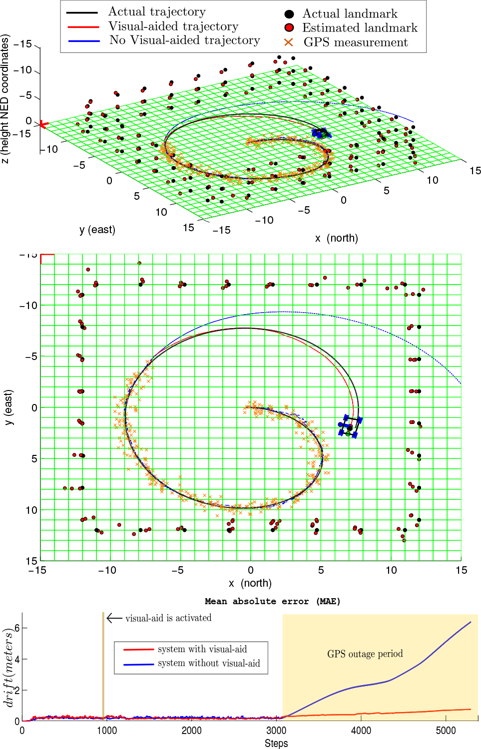
Figure 7 shows the map and trajectory obtained for the entire data set. This route has a longitude of 524 and an approximate duration of 320. In the original data set, there is GPS availability almost over the whole trajectory. Nevertheless, GPS outages were artificially introduced in order to test the performance of the method under visual-based navigation conditions. In this case, the system has been able to determine the actual trajectory of the vehicle fairly well, even in periods where the GPS signal is not available. Figure 8 shows two different instances corresponding to periods when the system is working without a GPS signal (i.e., visual-based navigation mode). The spatial significance of the map can be appreciated. It is important to note that the video sequence, which is used in this experiment, contains a few dynamic elements, such as a few pedestrians or a moving car. There is also a lot of variation in lighting conditions, which are typical in outdoor environments.

Map and trajectory estimated for the entire data set. Segments, in which the GPS is available, are indicated in blue; however, most of the trajectory was determined in visual-based navigation mode.
Estimated trajectory and map, corresponding to two different instants of time during periods of visual-based navigation. Visual features
5. Conclusion
In this work, a practical method for implementing a visual-aided inertial navigation and mapping system for autonomous robots has been presented. The testing of the method has been performed over real data collected from a land robot. However, it should be straightforward to extend the application of the method to other kinds of autonomous robot (e.g., flying robots).
A novel scheme has been introduced for taking advantage of visual information provided by a monocular camera. The proposed technique allows for handling, in an efficient and robust manner, the measurements corresponding to visual features. Experimental results, obtained through simulations and also with real data, show that the proposed method is able to estimate the trajectory of the vehicle fairly well, even in periods where the GPS signal is not available. In this case, the drift in estimation is considerably minimized, especially when it is compared with the results obtained using inertial sensors only. It is important to highlight that, in experiments, a video sequence with a low resolution and a low frame rate was used. In addition, the proposed method can operate with a moderate number of visual features being tracked.
The proposed method, different from visual odometry approaches, makes it possible to estimate the spatial location of visual features, whenever possible. Both the appearance and spatial information provided by the system could be potentially used for multiple tasks in future versions of the system.
Filter-based methods are convenient when limited processing power is a concern. However, the computational cost of Kalman filters scale poorly in relation to the incremental size of the state vector. For this reason, the proposed method treats each map feature independently, instead of augmenting the system state vector, as it is common in monocular SLAM approaches. The above characteristics should mean that the method is suitable for application to robots with limited resources.