
Abstract
This paper analyses the formation tracking of groups of mobile robots moving on the plane. A leader robot is chosen to follow a prescribed trajectory whilst the rest, considered as followers, are formed in an open-chain configuration. Two formation-tracking control laws using approximate velocities are proposed, in which some velocities must be communicated between robots in order to ensure the simultaneous preservation of the formation and the following of the group path. The main result is analysis of the convergence of the two proposed control laws. The restriction of inaccurate information occurs in decentralized multi-robot platforms, in which the mobile agents are only able to measure positions and the velocities' functions are estimated using online numerical methods. A numerical simulation of both controllers in the case of omnidirectional robots is shown. For the case of the unicycle-type robots, real-time experiments of both controllers were implemented and tested.
1. Introduction
Recently, the motion coordination of multiple biological entities has inspired the design and implementation of natural behaviours in mobile robots for industrial and service applications [1, 2]. Observations of ethologists have determined that the ordered motion of ants, fishes or birds is constructed from local interactions between mobile agents. Each agent acts according to the local information acquired from other members [3]. Therefore, the control schemes are decentralized and the study falls within the research areas of multi-agent systems, sensor networks and distributed control systems. The decentralized schemes also permit more autonomy for the robots, a smaller computational load in control implementations and the method's applicability to large-scale groups [4].
A special case of motion coordination is formation tracking [4, 5], also called marching control [6] or flocking behaviour [7], in which a group of mobile robots achieves geometric patterns whilst the whole group follows a prescribed marching trajectory. Formation tracking appears in some applications such as the transportation and manipulation of large objects, search and rescue tasks and perimeter detection, etc. In formation tracking, it is required that the group follows some trajectories in the workspace, while a rigid formation pattern is preserved simultaneously. Thus, the main challenge of formation tracking is the inter-robot strategic sharing of information about the marching path or the velocities of certain robots in the group, in order to ensure the formation's preservation, maintaining the greatest possible level of decentralization.
The leader-follower schemes [8, 9] are frequently studied by the academic community due to the inspiration that biological behaviour creates (for instance, in ants). In these schemes, a unique leader robot follows a marching path while the rest, termed followers, converge to some formation pattern with respect to the leader. Although some contributions have been proposed in relation to formation tracking, most of the studies consider that the robots can measure the exact information about the velocities of the other robots or the marching path. For instance, [10] studies the case of a convoy-like formation, in which the robots are initially placed at the desired positions, and they know the linear and angular velocities of the adjacent robot. The positions and orientations of virtual leaders serve as reference points for the follower robots in [11, 12] and the exact marching path derivative is available to all robots in [6, 5].
Note that in the natural leader-followers scheme, each agent is able to sense the position of only the nearby agents, and the velocities must be estimated or intuited by their local controllers. As will be discussed below, if some velocities are not approximated in the control laws, then the formation is not rigid during the path following, as shown in [13, 14], in which the positions of the followers vary in a ball that is centred in terms of the leader's reference frame. Some papers estimated the leader's velocity using position measurements acquired through observers [15] or local sensors [16]. The problem of formation tracking is studied via an estimator designed to track a globally desired velocity that is available to a subset of robots via a consensus-based velocity term in [17]. Predictive control is applied in [18], which added a term to the cost function of the leader in order to preserve the formation. Other works focus on the reconstruction of the marching path using adaptive algorithms in [19, 20, 21, 22], and Lyapunov techniques in [23]. The velocities of neighbours are estimated in [24, 25] in order to construct the desired marching path based on local information. Recently, the approximation of velocities for the case of spacecraft formations was obtained by using a non-linear filter with finite-time convergence in [26]. Most previous works designed estimation methods for the velocity of the agents based on the measurement of the marching path's exact velocity, decreasing decentralization and simplicity of the control laws. Commonly, some numerical methods are included in order to estimate velocities in the experimental platforms of multi-robot systems. However, the effects of these approximations have not been formally analysed.
In [27], two formation-tracking control laws were designed using exact velocity measurements in order to achieve formation-tracking convergence. This paper shows the boundedness of the formation-tracking error when only position information is used. The variation of the formation-tracking error can be made arbitrarily small when the approximations of velocities are close to the real values. In addition, for a class of tracking trajectory, we show the exponential convergence of the formation-tracking error. This study is important, since this is the way that such implementation is usually done. Nevertheless, the degradation of the performance on the overall system has not been formally studied. To show the effects of the approximate velocities, the control laws were extended to unicycle-type robots in real-time experiments.
The rest of the paper is organized as follows. Section 2 introduces the kinematic model and the problem statement. A short summary of our previous formation-tracking control strategy, with its exact velocities, is presented in Section 3 with numerical simulations. The main result of the paper is given in Section 4, using approximate velocities with numerical simulations. The extension of the model to unicycle-type robots and the real-time experiments are shown in Sections 5 and 6, respectively. Finally, some concluding remarks are presented in Section 7.
2. Problem Definition
Denote by N = {R1,…,Rn}, a set of n point robots moving in the space with positions zi(t) = [xi(t),yi(t)] T , i = 1,…,n. The kinematic model of each agent or robot Ri is described by

where
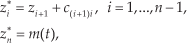
where
Figure 1 shows an example of formation tracking in which the robots satisfy a specific formation pattern while simultaneously following the trajectory m(t). The goal of the leader is to follow the marching path, whereas the goal of the followers is to maintain a desired pattern formation with respect to the leader, using the position of the adjacent robot as a guide. This strategy is usually considered as an open-chain or convoy configuration [10]. Note that the marching path could be constructed online by a human operator, who controls the displacement of the leader remotely while the followers achieve a formation.
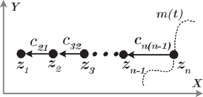
Desired formation tracking of the robots
Problem Statement. The goal of formation tracking is to design a control law ui = fi(zi,zi*) for every robot Ri, such that
3. Control strategy based on the exact information of velocities
Based on [27], for every follower robot, Local Potential Functions {LPFs) are defined by

Note that γ i is always positive and reaches its minimum only when zi = zi*. The standard approach of (attractive) LPFs consists in applying the partial derivative of an LPF with respect to zi, as control inputs of every robot Ri. Thus, the control inputs steer every robot to achieve the minimum of this potential function, which is designed according to the specific position vectors that construct a particular formation. Using these functions, two control laws can be defined by

where k,km>0. Note that the control law Γ1 requires the provision of feedback ṁ(t) to all followers, and that Γ2 includes the feedback of the adjacent robot żi+1 for all followers. Thus, the first n - 1 robots are not required to process complete information about m(t) or the positions of all robots, unlike in [4] or [28], in which all robots must know the target position or trajectory, and more than one desired distance between robots. A schematic description of the control strategies is shown in Fig. 3. Observe that the control law of the leader requires the exact derivative of m(t) to function, whilst the followers require the full knowledge of ṁ(t) or żi+1.

Formation-tracking scheme with the exact information about the velocities of robots and the trajectory

Formation-tracking scheme with the exact information of velocities
With respect to the convergence of the desired formation tracking using (4) or (5), the next proposition can be found in [27].
A sketch of the proof is included for completeness.
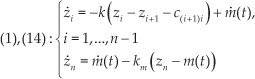
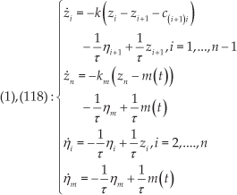
Proof. The dynamics of zi in the closed-loop systems (1), (4) and (1), (5) are given, respectively, by
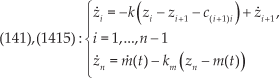
Define the error variables by

where e1,…,en-1 are the formation errors of the followers and en is the path-following error of the leader. The dynamics of the error coordinates (8) for the two control laws are given respectively by


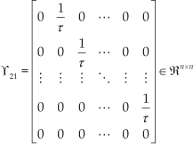
where ⊗ denotes the Kronecker product (the Kronecker product allows use of a more compact notation for the equations), I2 is the 2 × 2 identity matrix and the matrices B1 and B2 are

Clearly, the matrices B1 and B2 are Hurwitz ones, and the errors converge to zero. This means that the n – 1 first agents converge to the desired formation, whereas Rn converges to the marching path.
The control strategies (4) and (5) are appropriated for any kind of sufficiently smooth function m(t). Figure 3 shows a numerical simulation of both control laws with n = 3, k = 1 and km= 1. The initial conditions are given by z1(0)=[-1,3], z2(0)= [2, 2] and z3(0)=[2, 5]. The desired formation is a triangle defined by the vectors c21= [0, −4] and c32 = [-3,2], and the marching path is a circular path given by m(t)= [3 + cos(0.2t),3 + sin(0.2t)]. Note that the follower robots converge to the desired formation and that the leader robot, z3 (represented by a green dashed line), converges to the marching path m(t). This is shown through the convergence of the error variables. However, the two control laws present differences in the transitory regime.
The convergence of the errors is reached due to the strong assumption that both the velocities of the robots and the marching path are measured exactly. The requirements of the local controllers that the robots include these velocities can be translated into a greater overhead on the communication between the mobile agents. This is the reason motivating analysis of the impact of the velocities' approximation, which is addressed in the next section.
4. Control strategy using the approximations of velocities
Recalling the inspiration derived from nature, in which the mobile agents are capable of sensing only the position of the robots and the marching path, the two control schemes are now modified according to Fig. 4. The robots are not equipped with velocity sensors, and the control laws given by the equations (4) and (5) must be modified in order to incorporate some approximation method for estimating these velocities. The impact of these inexact data on the convergence analysis needs to be studied; hence, a modelled description of the approximation of the derivatives in the system's dynamics is included.
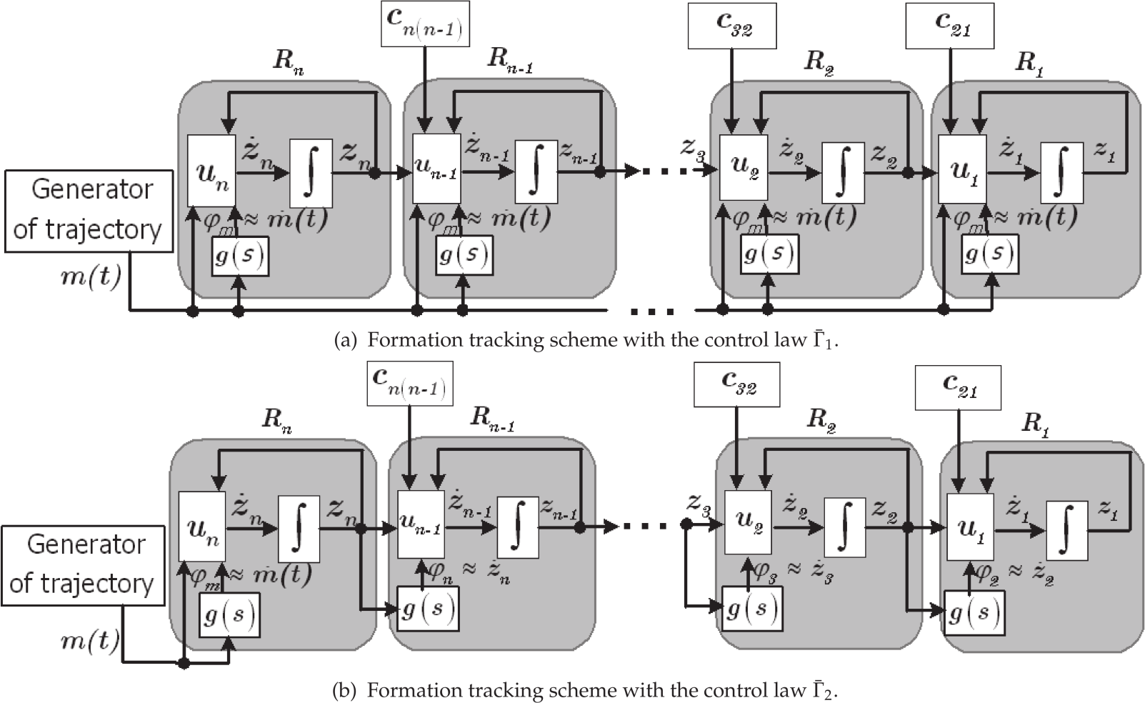
Formation-tracking scheme, with approximate information about the velocities of robots and the trajectory
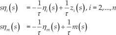
Note that the leader robot needs to approximate the derivative of m(t) and that the follower robots also need to approximate the velocity of the marching path (Figure 4 (a)) or the adjacent robot (Figure 4 (b)). In actual implementations, the velocities are calculated by the local controllers using numerical methods, performing a more realistic and decentralized scheme. The derivative approximation function shown in Fig. 4 is defined in the frequency domain as

where τ ɛ ℜ and τ ≥0. Thus, the approximation of velocity for a robot Ri and the trajectory m(t) is established by

Substituting (11) in (12), we obtain

By defining the auxiliary variables

it is possible to obtain from (14)
Therefore, by substituting (14) in (13), and using the inverse Laplace transform on (13) and (15), we can obtain the following differential equations

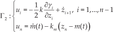
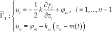
Considering the dynamics of the approximate velocities, the control laws Γ1 and Γ2 are modified as

The closed-loop systems (1), (17) and (1), (18) result in the extended system's equations

and, when written in matrix form, the closed-loop systems are given, respectively, by
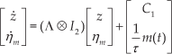

where

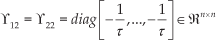
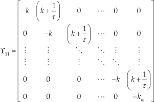
and

It is clear that, due to inexact information regarding the velocities, the errors converge to a residual set around zero, which depends on the quality of the approximate velocities. Similar to the previous case, it is necessary to analyse the convergence of the robots to the formation tracking. Thus, we define the following auxiliary variables

where the errors ei are similar to (8) and the δ i errors are the difference between the approximate velocities of the robots and the marching path. Note that if the errors ei converge to zero, the robots achieve the desired formation and the convergence of δ i ensures that the robots move at the same velocity as that of the marching path, i.e., preserving the formation pattern.
The next proposition is our main result, which establishes the boundedness of the errors around zero, based on small values of τ and the behaviour of the acceleration of the marching path.
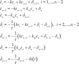
Proof. For the closed-loop system (1), (17), the dynamics of the error coordinates is given by

and written in matrix form as

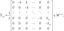
where

By using mathematical induction, it can be shown that the characteristic polynomial of matrix is given by p(λ) = (λ + k)2(n-1)(λ + km)2 + (λ + 1/τ)2; therefore we conclude that (24) is bounded-input, bounded-state stable.
On the other hand, for the closed-loop system (1), (18), the dynamics of the errors is given by
and written in matrix form as

where
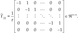
Now, the characteristic polynomial of matrix is given by p(λ) = (λ + 1)2n(λ + k)2(n-1)(λ+km)2; therefore we also conclude that (26) is bounded-input, bounded-state stable. In this case, observe that the eigenvalues do not depend on the value of τ.
Note that if m̈(t)=0, then we have a homogeneous, linear system in both cases; therefore, the solution converges exponentially to zero. Finally, the solution of the coordinate δn+1, as t → ∞, is bounded by

from which we can see that
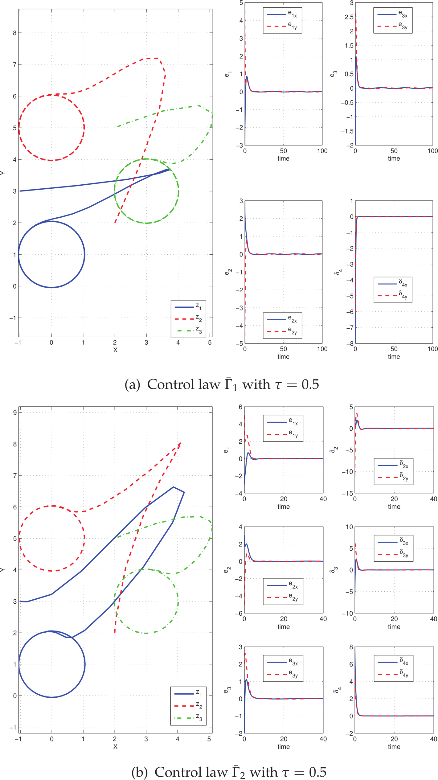
Figure 5 shows a numerical simulation of the closed-loop systems (1), (17) and (1), (18), with τ = 0.5, and the same parameters and initial conditions as in Fig. 2. The error coordinates do not converge to zero, but remain bounded around zero. The transitory regime is more evident than in the case of exact information.
IRobot Create
Analysing the effects of the gain parameter τ, define the error performance index in both cases as
Error-performance index with different values of

5. Extension of the control laws to the case of unicycle-type robots
The control laws (17) and (18) can be extended to the case of nonholonomic mobile robots. Consider the kinematic model of unicycle-type robots, as shown in Figure 6, given by

Simulation of formation tracking using approximate velocities

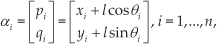
where vi and wi are the linear and angular velocities, respectively, of the midpoint of the wheel's axis given by (x,y). It is known that the dynamical system (28) cannot be stabilized by application of a continuous time-invariant control law [29]. Because of this restriction, the selection of the coordinates α i = (pi,qi), as shown in Figure 6, as a control output instead of (x,y) helps to simplify the analysis, avoiding singularities in the control law. Moreover, the position of the α i could be the position of an actuator or the robot's center of mass. The coordinates α i are given by
and their dynamics can be obtained as

where Ai(θ i ) is the so-called decoupling matrix of the robot Ri. Note that det(Ai(θ i ))=l ≠0. Therefore, it is possible to design a control strategy in order to move α i to a desired location using the control law [vi,wi] T = Ai−1(θ i ) fi,i = 1,…,n, where functions fi are the desired dynamics of the coordinates α i .
Thus, extending the previous results to the case of point robots, the control laws with exact velocities given in (4)-(5), or the control laws with approximate velocities expressed in (17)-(18), could be rewritten for unicycle robots by

where ūi are identical functions of the control laws ui as defined in (4)-(5) and (17)-(18), depending on the coordinates αi. Note that the dynamics of the coordinates α i in the closed-loop system (29)-(31) are reduced to α i = ūi, i = 1,…,n. Therefore, the analysis of the formation tracking becomes in the case of holonomic robots studied in Sections 3 and 4. Note that these input-output linearizations leave the orientation angles θ i in an uncontrolled state.
6. Experimental work
The control strategies were implemented using an experimental set-up consisting of three unicycle-type robots manufactured by IRobot, the model Create, and a vision system comprising a monochrome camera Genie HM-1024 with an Ethernet communication, developed by Teledyne Dalsa. The camera captures the position of two white circle marks placed on top of every robot, as shown in Fig. 5, indicating the coordinates (xi,yi) and α i . The camera is installed at a height of 2.5m and configured to work at 117 frames per second. Therefore, the sampling period is given by 8 milliseconds and the resolution of the camera is given by 1024×768 pixels which produces a position resolution of 3mm2 per pixel. Note that both the workspace and the robots are covered in black in order to highlight the white markings.
Using the white marks, the position and orientation of every robot is calculated using a Core i5 PC with 4GB RAM. The same computer subsequently evaluates the control laws and generates the control signals ui and wi for every robot, which are transformed into the desired angular velocities for the robot wheels, by


where wri and wli are the right and left wheel of each robot, respectively, L = 0.25m is the distance between two wheels and r = 0.03m is the radius of the wheels. Finally, the desired angular velocities are sent via a wireless Bluetooth transmitter to every robot. The image processing and the control law were developed in a software application using the real-time programming of Matlab R 2013a.
Note that the experimental set-up becomes a flexible platform for emulating different formation-tracking systems, from centralized to decentralized schemes, by selecting the adequate information obtained from the vision system to be used in the local control laws of each robot.
To complement the control laws, a reactive secondary control law for the avoidance of inter-robot collision was programmed into the experiments. Although the prevention of possible collisions was achieved using a simple reactive control law, in the experiments, none of the robots were in danger of collision due to their initial conditions. The analysis of non-collision in formation tracking is not studied in this paper and will be addressed in further research.
6.1 Experiments with exact velocities
Figure 8 shows an experiment of the control law Γ1 given in (4) using the exact information of the derivative of m(f), with n = 3, k = 1, km = 1 and l =0.15m. The marching path is the circle given (in metres) by

Kinematic model of unicycles

Experiment 1 using the control law Γ1
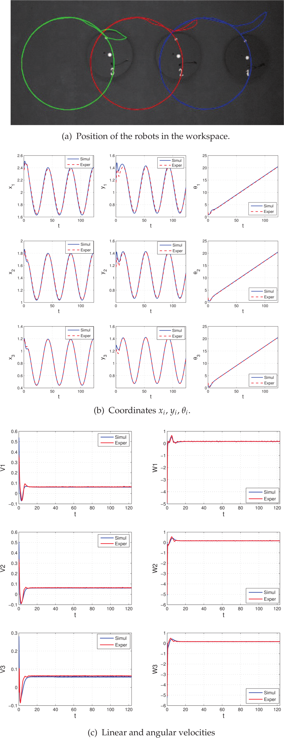
The second experiment is given in Figure 9, which is now dedicated to the control law Γ2 given in (5) using the exact information of the robots' velocities. The value of the control gains k and km are similar to the ones used in the previous case. Now the robots are formed in a triangular shape, given by the vectors c21 = [0.6,0.6] and c32 = [0.6,-0.6], The initial conditions are [x1,y1,θ1] = [2.26,0.70,1.68], [x2,y2,θ2] = [2.03,1.45,2.85] and [x3,y3,θ3] = [1.03,0.65,0.68]. The trajectories of the coordinates α i that are recorded by the vision system are presented in Figure 9(a). The evolution of xi, yi and θ i is depicted in Figure 9(b). The control outputs vi and wi are shown in Figure 9(c). Similar to the previous case, the graphs show a good performance of the control law, in which the robots converge to the desired formation tracking and the experimental results are close to the numerical simulation.

Experiment 2 using the control law xi
In both experiments, the orientation angles converge to the same value although they are not controlled by the control laws. In addition, note that the linear and angular velocities shown in Figures 8(c) and 9(c) converge to a positive value; therefore, the robots after the transitory regime, continue to move in an antoclockwise direction while facing the front. It is shown in Figures 8(b) and 9(b) where the trajectories of coordinates yi and Γ2, respectively, describe the parametric functions of the circumference, and that the orientation angles are positive and increasing.
The quantization error is considered to be sufficiently small for this experiment, due to the precision of the camera and the insignificance of its influence. This can be seen in Figures 8 and 9, where the results show a ripple in the order of the instrument's resolution.
6.2 Experiments with approximate velocities
Figure 10 shows an experiment 3 using the control law
Experiment 3 using the control law
Finally, the fourth experiment is given in Figure 11, using the control law

Experiment 4 using the control law
Note that the trajectories in Experiments 3 and 4 are modified due to the approximations of the velocities and the performance of the robots deteriorating with respect to the ideal case. The transient response of the control inputs, as shown in Figures 10(c) and 11(c), exhibits a larger overshoot with respect to the control inputs of Experiments 1 and 2, as presented in Figures 8(c) and 9(c), respectively, with the worst being Experiment 4. Similar to Experiments 1 and 2, the linear and angular velocities converge to a positive value; therefore, the robots continue to move in an antoclockwise direction while facing the front, which is verified by the trajectories depicted in Figures 10(b) and 11(b), respectively.
According to the main result detailed in Section 4, the errors remain oscillatory around zero. These effects are shown in Figure 12 for Experiments 3 and 4, respectively. Note that due to propagation of the inexact measures of velocities along the chain of robots, the behaviour of the errors worsen in robots that move away from the leader. Thus, the robot R1 exhibits the worst performance in the formation tracking.

Graphics of errors using approximate velocities
7. Conclusion
This paper shows that, assuming perfect knowledge about the positions and velocities of the robots and the marching path, it is possible to guarantee the preservation of a rigid formation and the group trajectory tracking of the robots. However, during a decentralized formation tracking, the robots measure only positions and the velocities must be approximated. This paper incorporates the analysis of the variables of approximate velocities within the closed-loop systems, and some conditions are determined in order to ensure that the errors are bounded. The desired outcome occurs if the trajectory is sufficiently smooth and the bound of the errors' performance improves when the bandwidth approximation increases for the velocities, recovering the ideal case in the limit. The control laws were extended for the case of unicycle-type robots with numerical simulations and real-time experiments. In further research, the analysis of control strategies with other formation-tracking topologies and collision avoidance applied to different nonholonomic mobile robots will be studied.
Footnotes
8. Acknowledgements
The authors kindly acknowledge the financial support of the Universidad Iberoamericana and the Universidad Católica del Uruguay.