Hybrid Architecture for Coordination of AGVs in FMS

Abstract

This paper presents a hybrid control architecture that coordinates the motion of groups of automated guided vehicles in flexible manufacturing systems. The high-level control is based on a Petri net model, using the industrial standard ISA-95, obtaining a task-based coordination of equipment and storage considering process restrictions, logical precedences, shared resources and the assignment of robots to move workpieces individually or in subgroups. On the other hand, in the low-level control, three basic control laws are designed for unicycle-type robots in order to achieve desired formation patterns and marching behaviours, avoiding inter-robot collisions. The control scheme combines the task assignment for the robots obtained from the discrete-event model and the implementation of formation and marching continuous control laws applied to the motion of the mobile robots. The hybrid architecture is implemented and validated for the case of a flexible manufacturing system and four mobile robots using a virtual reality platform.

1. Introduction

Currently, some production systems require the coordination of automated Flexible Manufacturing Systems (FMS) for the assembly of different and concurrent products [1]. Petri net (PN) formalism have been widely applied to modelling and supervisory control for FMS [2, 3]. The structure and properties of a PN can represent the asynchronous actions, blocking, concurrency and other dynamic behaviours that frequently appear in large FMS [4, 5].

The Material-Handling System (MHS) is crucial for the productivity of an FMS. This transports the workpieces between storage locations and workstations, and is composed commonly of conveyor belts or manipulators mounted in rails. This kind of MHS becomes fixed and non-reconfigurable transport setup, which could be inadequate for highly flexible manufacturing systems, where new routes could appear in some product sequences. To increase the flexibility of the MHS, several studies have recently appeared in the control systems community on the implementation of groups of mobile robots or Automated Guided Vehicles (AGVs), emulating the coordinated work achieved by a group of workers. An example of groups of robots in a manufacturing industry is the Kiva system [6, 7], where mobile storage locations are charged and moved by small autonomous robots; the human operators remain standing while the products come to them. In [8], the Kiva system includes information about inventories and work orders. The collective behaviour of groups AGVs presents some advantages such as redundancy and fault tolerance when a robot is broken, and the loading of large objects by subgroups of robots in specific formation patterns [9].

A coordinated control of AGVs in an FMS must enable group behaviours like formation control, path following maintaining a formation pattern (marching), and collision avoidance between robots or static obstacles [10]. Also, this coordination must obey process specifications, fault-tolerance strategies and the assignment of routes according to some rules of distances or equitable energy distribution [11]. In terms of the continuous dynamic behaviour of multi-robot systems, the coordination of AGVs has been mentioned by the control systems community as a possible application of the generic problems of consensus, formation control, marching control, collision avoidance and dispersion [12]. The control schemes encompass behaviour-based control laws [13], swarm stability [14], virtual structures [15], leader-follower schemes [16], and artificial potential functions [17]. The case of coordination of unicycle-type robots to achieve formation and marching behaviours has been widely studied by the robotics community due to the drawbacks of non-holonomic restrictions. For example, distributed control laws with limited information for the group tracking of a predefined path are proposed in [18], motion coordination control algorithms for convergence to a desired geometric pattern using are given in [19], stabilization of distributed local tracking is analysed in [20], and a biology-inspired decentralized navigation law with limited information about other robots in the group is designed in [21].

Despite the importance of analysis of the performance of control laws for point robots and unicycle-type robots, no previous work has clarified how these low-level control strategies can be applied to the case of manufacturing systems, or their interconnection to a coordination layer of tasks for robots within a production system. A few works, like [22], propose some hybrid architectures of formation control and a planning level, in this case neural networks, for dispersion tasks. Despite the potentiality of multi-robot mobile systems in FMS, mobile robots researchers have focused only on the design of generic control laws related to the formation, marching and collision avoidance of groups of robots in experimental platforms, assuming that these behaviours can be adopted in an industrial context, which must operate under the requirements of industrial standards such as ISA-95 [23]. On the other hand, the discrete-event community has studied only the high-level behaviour of FMS, excluding the analysis of the motion of the AGVs [24, 25]. There are few recent studies on the combination of discrete-event models and multi-agent robot systems. For example, in [26] a PN model coordinates some agents in computer systems while avoiding deadlock. A new type of agent-based PN is defined in [27, 28] for the communication of computer systems. Finally, a supervisory control for Finite State Automata using AGVs is obtained for an FMS in [29], where the drawback of state explosion is presented in a real scenario.

This paper proposes a hybrid architecture that models an FMS using PN in a high-level coordination. The PN model represents the concurrency of tasks, the logic of precedence between tasks, the limitation of storage and the availability of robots. In the low-level coordination, the control selects adequate AGVs to transport the pieces and implements continuous control laws to achieve formations, marching behaviours and collision avoidance of groups of robots. The approach clarifies the overlap between the two control levels, facilitating implementation in engineering practice.

The paper is organized as follows. Section 2 presents the problem statement. Section 3 summarizes the main concepts of PN. Section 4 presents the modelling framework of PN for the FMS. Section 5 defines the formation, marching and collision avoidance control laws for the AGVs. Section 6 presents the case study of four AGVs moving in an FMS. Finally, Section 7 presents some concluding remarks.

2. Problem statement

A general scheme of an FMS is presented in Figure 1 (see [1]), composed of a set of raw material storage locations, which provides workpieces for a set of machines, commonly Computer Numerical Control (CNC) machines, which can be programmed to perform different machining of the same raw material. The manufactured pieces of every machine are moved to specific slots in intermediated storage. Commonly, the intermediated storage is installed in matrix-shaped storage locations, where each row contains the parts manufactured by the same machine. When a product is required, the adequate number and type of parts contained in intermediate storage are transported to the assembly stations where different assembly programmes are carried out. The final assembled products are moved to final product storage and the FMS becomes available for other subsequent processes. A set of homogeneous AGVs are added to the system to transport the raw material, machined parts or final assembly products between the different equipment of the FMS. Note that, in a general case, one or many workpieces could be transported by one or many AGVs, enabling formations of robots in specific geometric patterns and group following of routes in the workspace. As shown in Figure 1, the AGVs are initially in a home position, where the robots can be connected to a battery charging station. When a robot finishes a task, it can return to its home position or attend to another transportation task.

Figure 1.

General scheme of an FMS

The main objective is to design control architecture that coordinates the AGVs and the process tasks, achieving maximum concurrency and obeying process restrictions in a general FMS. The PN must achieve process task ordering, equipment and storage availability representation and assignment of AGVs for the transportation of workpieces. On the other hand, the robots must receive the necessary information to implement formation, marching and collision avoidance control laws for group transportation of pieces. The next section describes the basic PN principles that need to be observed to analyse the general modelling of an FMS with AGVs.

3. Petri Net basic definitions

Definition 1: According to [2, 3], a PN with finite capacity is a weighted and bipartite graph given by a 5-tuple

$PN=\left(P,T,F,W,M_0\right),$

(1)

where:

• P = {p₁, p ₂ ,…p _m } and T = {t₁,t₂, …,t _n } are the disjoint sets of nodes called places and transitions, respectively.

• F ⊆ (P × T) ∪ (T x P) is the set of arcs, connecting places to transitions and vice versa, with elements w(p,t),w(t,p), ∀t ∈ T, ∀p ∈ P.

• W:F→Z ⁺ is the function that assigns the weights to each arc.

• M(p): P→Z⁺, represents an m-entry vector with the number of tokens residing inside each place. Let M₀ be the initial marking, and consider that eachp _i ∈ P has a finite capacity c_i of tokens; then, M(p _i ) ≤ c _i .

The reachability R(PN) is the set of all possible markings reachable from M₀. A k-th state or marking in a PN, denoted by M_k is achieved according to the following transition rule.

Definition 2: A transition t_i ∈ T is said to be enabled in a PN with finite capacity if:

M _k (p _j ) ≥ w(p _j ,t _i ), ∀p _j |w(p _j ,t _i ) ∈ F, with j=1,…,m and i=1,…,n.

w(t _i ,p _j )+M _k (p _j ) ≤ c _j , ∀p _j ∈ P.

If t_i is enabled in the k-th firing in some firing sequence, then the next marking is defined by

${\mathrm{M}}_{\text{k+1}}{\text{(p}}_{\mathrm{j}}{\text{)=M}}_{\mathrm{k}}{\text{(p}}_{\mathrm{j}}{\text{)-w(p}}_{\mathrm{j}}{\text{,t}}_{\mathrm{i}}{\text{)+w(t}}_{\mathrm{i}}{\text{,p}}_{\mathrm{j}}\text{)}$

(2)

4. PN modelling framework for the FMS

4.1 Definition of storage locations, machines, assembly stations and process tasks

According to the problem statement presented in Section 2, consider PM = {PM₁, …,PM_n} as the set of process machines (PM), AS = {AS₁, …, AS_m} as the set of assembly stations (AS) and AGV = {AGV₁, …, AGV_r} as the set of AGVs. It is assumed that each PM_j, i = 1, …,n performs M_i1, …, M_ik. machining programmes. Every machining M_ij with i = 1, …, n,j = 1, …, k_j requires the raw material contained in the raw material storage locations (RM) RM_ij. The RM_jj is manually loaded and has a capacity limited to C(RM_ij) pieces. When the machining M_ij has finished, the manufactured part is allocated to an intermediated storage location, numbered as IS_ij with a capacity limited to C(IS_ij). Denoted by A₁(RM_ij,PM_i,n_ij) is the AGVs' task of transporting a raw material from RM_ij to PM_i using n_ij ≤ r AGVs to perform the machining M_ij and denote by A₂(PM_i, IS_ij,m_ij) is the task of transporting the manufactured parts of the machining program M_ij from PM_i to IS_ij using m_ij ≤ r mobile robots. Note that m_ij ≤ n_ij because the machining M_ij generally removes material from the workpiece, decreasing the dimension and weight of the manufactured part. If n_ij,m_ij > 1, this implies that the robots achieve a formation control and path following that will be detailed in the next section.

Each assembly station AS_p,p = 1, …, m performs ${\mathrm{S}}_{\text{i1}}\text{,}\mathrm{\dots }{\text{,S}}_{{\text{ir}}_{\mathrm{p}}}$ assembly programs. Each S_pq with p = 1, …, m, q = 1, …, r_p assembles the parts allocated to the different intermediate storage locations. Let ${\text{U(S}}_{\text{pq}}\text{)}\subseteq {\text{{IS}}_{11}\text{,}\mathrm{\dots }{\text{,IS}}_{{\text{nk}}_{\mathrm{n}}}\text{}}$ be the set of intermediate storage locations that contains the parts needed to complete the assembly program S_pq and K(S_pq, IS_ij) ∈ Z⁺, ∀IS_ij ∈ U(S_pq) the quantity of parts of IS_ij to achieve the assembly program S_pq. Then, we define A₃ (IS_ij,AS_p,m_ij) as the task related to the transportation of a part from IS_ij to AS_p to perform the assembly program S_pq using the same m_ij number of AGVs. Note that the previous task must be repeated K(S_pq, IS_ij) times, but not necessarily by the same robots. Finally, when the assembly program S_pq has finished, then the final assembly product is placed in the final product storage location FP_pq, which has a capacity limited to C(FP_pq), and is manually unloaded. Denoted by A₄(AS_p,FP_pq,t_pq), the transportation of the final assembly product made by S_pq from AS_p to FP_pq now uses t_pq ≤ r robots. Figures 1 and 2 show schematically the storage locations, PM, AS and their process tasks, and the routes of the AGVs in the system, where the labels of some arrows are related to the number of pieces K(S_pq,IS_ij) moved by the robots. Note that A₁,A₂,A₃ and A₄ are the four kinds of transportation tasks realized by the AGVs.

Figure 2.

Scheme with process task

The PM, AS and AGVs can be classified using the reference model in the ISA-95 standard [23], according to Figure 3, where a clear separation of the MHS (the AGVs) and the process workstations (machines and assembly stations) is proposed. Then, the process tasks are assigned to each equipment device, illustrated at the bottom of Figure 3. ISA-95 proposes that product sequences be reduced to the correct order of the process tasks (product recipe) commonly addressed in a computer-based system, avoiding the reprogramming of the routines in the local controllers of the FMS elements when a new product is required.

Figure 3.

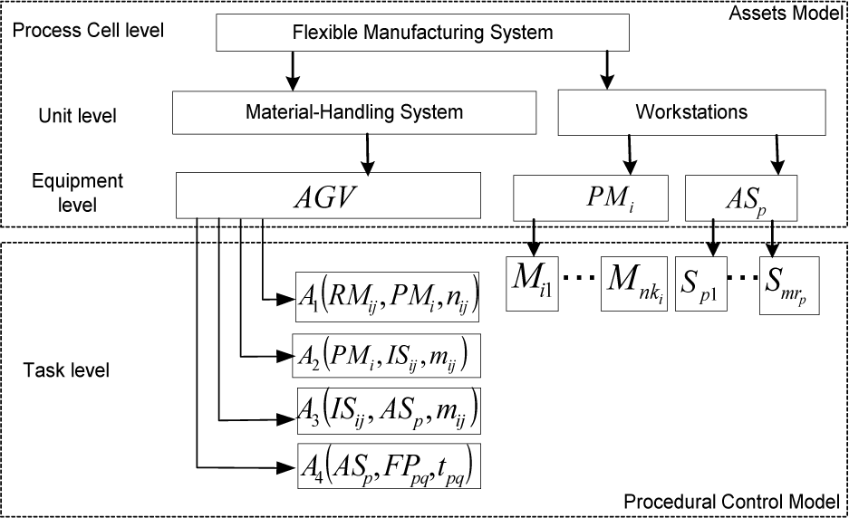
Equipment and task decomposition using the ISA-95 standard

Using the notation and terminology defined previously, some generic models of PN are constructed in order to obtain a general model of the FMS.

4.2 PN model of the system

Figure 4 presents a graphic representation, based on a precedence diagram, of the relationships between tasks (rectangles) and storage locations (circles). Note that each wide arrow symbolizes a relation between a storage location and material handling tasks performed by the AGVs, the continuous arrows are direct precedences and the dotted arrows represent inverse precedences between a pair of tasks.

Figure 4.

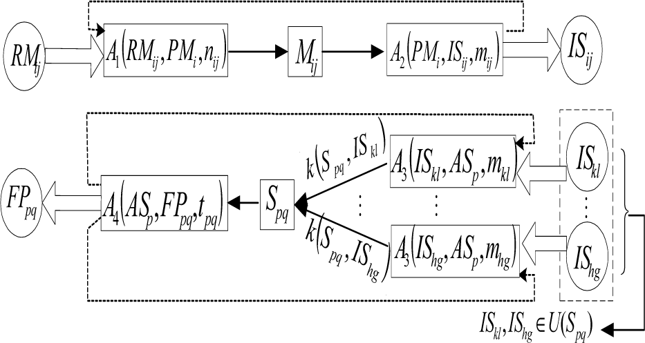
Logical precedences in a general FMS

The diagram in Figure 4 is divided into two sections. The first corresponds to the manufacture of parts. The AGVs transport the raw material from the storage RM_ij to the machine PM_i (for the machining task M_ij) through the task A₁; when the machine finishes, the AGVs transport the machined subpart from the machine PM_i to intermediate storage through the task A₂. The direct logical precedences between A₁ − PM_i and PM_i–A₂ establish that only when the precedent task ends does the subsequent task start. When the AGVs finish the task A₂, they can once again transport raw materials to the machine PM_i, avoiding conflict at the entrance of the machine. There are “inverse” logical precedences (dotted line) between A₂ − A₁, explained in detail in the next subsection. The second section of Figure 4 corresponds to the assembly operations. The subparts are transported from the storage locations IS_ij to the assembly station AS_p using the task A₃. Recalling the weight K(S_pq, IS_ij) establishes the number of necessary parts of the storage IS_ij to complete an assembly S_pq . When S_pq is finished, the final product is transported by the AGVs to storage FP_pq through a task A₄. Finally, there is an inverse dependence of A₄ − A₃, which ensures that the AGVs reload the assembly station only when the previous product has been stored in FP_pq.

4.3 Basic PN models

The relations between the storage locations and tasks, as presented in Figure 4, can be reduced to (1) the process tasks, (2) unloading or loading at a storage location, (3) the logical precedence (direct or inverse) between a pair of tasks, and (4) the conditions of gathering parts for an assembly and the starting of a new assembly. These relationships are examined below.

4.3.1 Tasks of AGVs, machines and assembly stations

Models of the tasks performed by the AGVs, machines and assembly stations are shown in Figure 5. The prefixes “s” and “f” denote the start and finish of tasks, respectively. The four types of AGV tasks (A_i, i = 1, …,4) shown in Figure 5a can be summarized as A_j(X,Y,w), where X denotes the place where the robots pick up the pieces, Y represents the place where the robots drop these pieces, and w is the quantity of robots needed to perform the task. The value of w is related to the type of transportation according to the table in Figure 5a. The number of AGVs is translated to the tokens in the place named AGV. Note that when a task A_i(X,Y,w) starts, the w tokens are removed from AGV and returned when the task finished. The selection of the AGVs assigned to each task could be performed according to the smallest distance of the robots with respect to the point where the robots pick up the piece.

Figure 5.

Models of tasks and translation PN

The machining and assembly tasks are represented in Figures 5b and 5c, respectively. Note that the places PM_i,AS_p contain one token, denoting that every machine or assembly station can carry out one process task at the same time.

4.3.2 Storage models

The storage models in the FMS are classified in three types: (a) manual load-automatic unload, as in dispensers of raw material (RM_ij) like entries of the FMS, (b) automatic load-automatic unload, for intermediate storage locations of subparts (IS_ij), and (c) automatic load- manual unload, which involves the storage of final products (FP_pq) when the products leave the FMS. The three kinds of storage models and their translation to PN are shown in Figure 6. In Figure 6a, the load of storage RM_ij requires a manual input transition IN_ij that puts tokens at RM_ij, which are extracted by the start of a task T_a ∈ A₁. In Figure 6b, storage IS_ij is loaded by the end of a task T_a ∈ A₂ and unloaded by the start of tasks T_b … T_c ∈ A₃. Finally, Figure 6c shows storage locations loaded by the end of a task T_a ∈ A₄ (final product) and unloaded by a manual transition OUT _pq that absorbs tokens from the place FP_pq.

Figure 6.

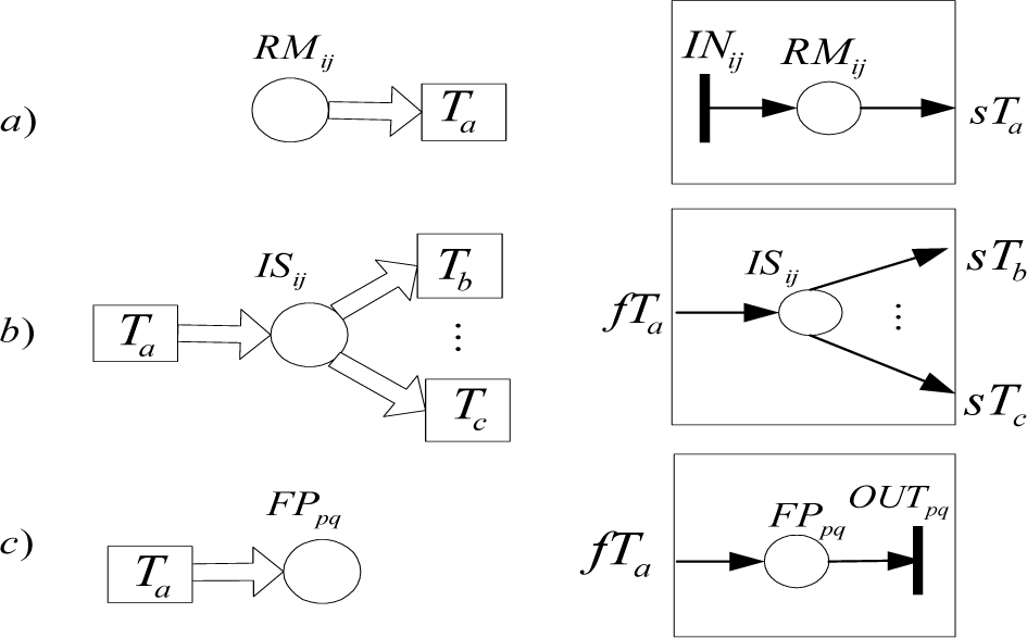
Storage models and translation PN

4.3.3 Logical precedences between tasks

The logical precedences represent the correct functional flow of the tasks during the FMS execution. There exist two basic kinds of precedences: direct logical precedences (D-direct) and inverse logical precedences (D-inverse).

A D-direct appears when, in the normal functional flow of the FMS operation, the finish of a previous task enables the beginning of a subsequent task. Figure 7a shows a simple graphical representation of a D-direct between tasks T_a and T_b, where the boxes are tasks (left side = start and right side = end). The PN translation of the D-direct is given in Figure 7b. Note that the initial marking is equal to zero.

Figure 7.

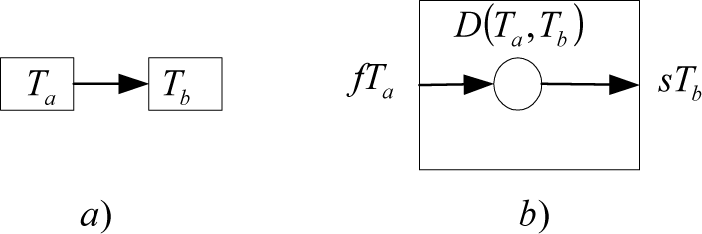
D-direct precedence models

A D-inverse occurs when the finish of a posterior task enables the start of an initial task, in a normal functional flow of the FMS, for example when the end of a machining task enables the feeding of a new part. Figure 8a shows a D-inverse, where the continuous line has been changed to a dotted line. Now, the end of the subsequent T_b enables the start of T_a The translation of a D-inverse to PN is shown in Figure 8b. Note that the tokens at the place of the D-inverse are not zero, because it is necessary to enable the beginning of the task T_a at the start of the functional flow.

Figure 8.

D-inverse precedence models

4.3.4 Logical precedences with multiple tasks

Extending the simple models of D-direct and D-inverse, we obtain general models for the conjunction of multiple tasks that enable the start of multiple posterior tasks. It appears for example in the case of transportation of subparts to enable the starting of an assembly task. Figures 7 and 8 can be extended to encompass the models in Figure 9a, showing the synchronization of two or more different tasks T_a … T_b ∈ A₃ required to achieve the start of an assembly task T_c ∈ S_pq. Note that K(T_c, IS_ij) is a weight added to each output arc denoting the number of subparts in IS_ij needed to start the task S_pq. Figure 9b shows an inverse dependence, where the end of task T_d ∈ A₄ allows the start of two or more tasks T_a … T_b ∈ A₃ for a new assembly. The PN translation needs the same quantity of places D as tasks T_a… T_b ∈ A₃; each place initially contains K(T_c, IS_ij) tokens representing the amount of necessary subparts for IS_ij for each assembly S_pq; the input arcs to the places D also have the weight K(T_c,IS_ij).

Figure 9.

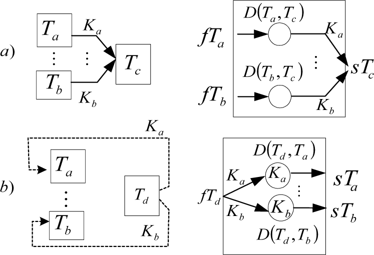
Logical precedences for the conjunction of different tasks

Applying the PN models of AGVs, machines, assembly stations, storage and logical precedences to the main diagram of the FMS shown in Figure 4, the result is a general discrete-event model with maximum concurrency of tasks. The case study shows in detail the translation of the PN models.

Remark 1: The modelling approach is a novel use of PN, based on the industry standard ISA-95. The rules of the PN evolution will serve as a high-level coordinator for the equipment and the mobile robots. The main contribution is to provide clarity for the construction of generic blocks and the interconnection to generate complex PN. This focus facilitates the study of real industrial FMS and its implementation in supervisory systems.

5. Coordination of the AGVs

In the previous section, the discrete-event dynamics of the FMS were modelled as a PN, where the task of motion of the AGVs is related to the quantity of AGVs that transport workpieces between machines, assembly stations and storage locations of the FMS. Thus, at a low level some motion control laws must be designed to achieve formations and to follow prescribed trajectories in the FMS. A brief introduction about the standard formation and marching control [30] is presented in the next subsection.

5.1 Kinematic models of AGVs

Denoted by N = {R₁,…, R_n}, a subset of n unicycles are moving in the plane. Note that n ≤ r, where r is the quantity of AGVs available in the FMS. The kinematic model of each agent or robot R_i, as shown in Figure 10, is described by

$\left[\begin{array}{l}{\stackrel{.}{x}}_i\hfill \\ {\stackrel{.}{y}}_i\hfill \\ {\stackrel{.}{\theta }}_i\hfill \end{array}\right]=\underset{R_i({\theta }_i)}{\underbrace{\left[\begin{array}{ll}cos{\theta }_i\hfill & 0\hfill \\ sin{\theta }_i\hfill & 0\hfill \\ 0\hfill & 1\hfill \end{array}\right]}}\left[\begin{array}{l}{v}_i\hfill \\ {\omega }_i\hfill \end{array}\right],i=1,\mathrm{\dots }n$

(3)

where v_i is the linear velocity of the midpoint of the wheels axis, ω_j is its angular velocity and R _i (θ _i ) the rotation matrix. In this work, we consider the position of the front point α_i = (p_i, q_i), shown in Figure 10 as the objective of control. This coordinate can be the centre of mass of the vehicle or the place where a sensor or actuator is placed. Also, the previous condition avoids singularities in the control law and facilitates the analysis simplification in the case of a point robot, as mentioned below [31, 32]. The coordinates αi, and their dynamics are given by

$a_i=\left[\begin{array}{c}{p}_i\\ q_i\end{array}\right]=\left[\begin{array}{c}{x}_i+\ell \cos ({\theta }_i)\\ y_i+\ell \sin ({\theta }_i)\end{array}\right],i=1,\mathrm{\dots },n$

(4)

${\stackrel{.}{a}}_i-\underset{A_i({\theta }_i)}{\underbrace{\left[\begin{array}{cc}\cos {\theta }_i& -\ell \sin {\theta }_i\\ \sin {\theta }_i& \ell \cos {\theta }_i\end{array}\right]}},i=1,\mathrm{\dots },n$

(5)

where A _i (θ _i ) is the so-called decoupling matrix of every R_i, which is non-singular because det(A_i(θ_i)) = 1 ≠ 0. Then, it is possible to design a control strategy for the positioning of α_i at a desired location using the control law

${[{\nu }_i,{\omega }_i]}^T=A_i^{-1}({\theta }_i)f_i,i=1,\mathrm{\dots },n$

(6)

where f _i is the desired dynamics of coordinates α_i. Note that in the closed-loop system (5)–(6), the dynamics of αi are reduced to ${\stackrel{.}{\alpha }}_{\mathrm{i}}{\text{=f}}_{\mathrm{i}}$ , and the behaviour of the front point is similar to the case of a simple point robot moving in the plane, cancelling all the non-linearities of the original kinematic model. Note that the control law (6) does not influence directly the orientation angles θ_i, but these could converge, as mentioned in [30]. The main objective of the control law is to design the functions f_i to achieve (1) formation, (2) convergence to a point, and (3) marching behaviour, avoiding inter-robot collisions in the three cases.

Figure 10.

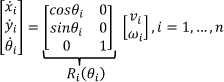
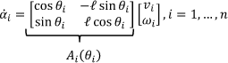
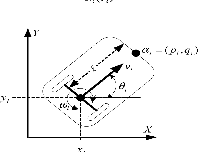
Kinematic model of unicycle-type robots

5.2 Formation control and collision avoidance

The main aim of formation control is to achieve a formation pattern defined by the relative positions of every robot with respect to team members. Let N_i ⊆ {α₁, …,α_n}, N_j ≠ Ø, i = 1,…, n denote the subset of positions of the robots which are detectable for R_j. If α_j ∈ N_i, then a relative position vector C_ji = [h_ji,v_jj] is defined which represents the desired position of α_i with respect to α_j in a particular formation. For a general case, the desired position of α_i with respect to all the detectable robots can be expressed by

$\begin{array}{l}{\alpha }_i^{*}=\frac{1}{n_i}\underset{j\in N_i}{\Sigma }({\alpha }_j+c_{ji}),i=1,\mathrm{\dots },n-1\\ {\alpha }_n^{*}=\frac{1}{n_n+1}(\underset{j\in N_n}{\Sigma }({\alpha }_j+c_{jn})+\tau )\end{array}$

(7)

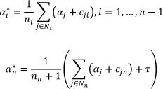
where n_j is the cardinality of N_j. Thus, the desired relative position of R_j can be considered as a combination of the desired positions of α_j with respect to the positions of all elements of N_j. Note that α*_n includes τ ∈ R², which denotes a reference point within the work area known by the n – th robot only (assigned as leader robot). The existence of a reference point is necessary to converge to a specific area of the workspace. It is clear that the position of i depends on the place where the storage locations and machines in the FMS are established.

The main objective is to design a formation control law for every robot R_i, such that lim_t→∞(α_j − α_i*) = 0, i = 1,…, n (convergence to the desired formation) and ||α_i(t) − α_j(t)|| > d, ∀t ≥ 0, i ≠ j (collision avoidance) where d is the diameter of a circle centred on the coordinate α_i that circumscribes each robot. According to [25], a formation control law with inter-robot collision avoidance is given by

$f_i=-\frac{1}{2}k\left(\frac{\partial {\gamma }_i}{\partial {\alpha }_i}\right)-\frac{1}{2}\eta \left(\frac{\partial V_i}{\partial {\alpha }_i}\right),i=1,\mathrm{\dots },n$

(8)

where k, η > 0 γ_i = ||α_i − α _i *||² is a (positive) attractive potential function with γ_i = 0 only when α_i = α_i*. The function V_i is the repulsive potential function, proposed by Khatib [26], defined between a pair of robots that violate the minimum allowed distance given by ${\mathrm{V}}_{\mathrm{i}}{\text{=Σ}}_{\mathrm{j}\in {\mathrm{M}}_{\mathrm{i}}}\left(\frac{1}{{\Vert {\text{α}}_{\mathrm{i}}{\text{-α}}_{\mathrm{j}}\Vert }^2}\text{-}\frac{1}{{\mathrm{d}}^2}\right)\text{i=1,}\mathrm{\dots }\text{,n}$ , where M_i = {α_j | ||α_i − α_j|| ≤ d}, i = 1, …, n . Note that every robot R_i always senses the position of the robots that belong to N_i, and eventually they can sense the closer robots using proximity sensors. The control law (8) describes an artificial vector field where the robots are attracted to the desired position and eventually avoid inter-robot collisions.

5.3 Convergence to a point in the plane

When a robot R_i requires only to converge to a static point β_i ∈ R², a modification of the control law (8) can be given by

${\tilde{f}}_i=-\frac{1}{2}k\left(\frac{\partial {\rho }_i}{\partial {\alpha }_i}\right)-\frac{1}{2}\eta \left(\frac{\partial V_i}{\partial {\alpha }_i}\right),i=1,\mathrm{\dots },n$

(9)

where ρ_i = ||α _i − β _i ||². The location of the point β_i, as mentioned below, could coincide with the home position of the robot, which includes a battery charge station.

5.4 Marching control

Assuming that the robots are formed in a desired pattern, [33] proposes the next marching control strategy, where the leader follows a desired marching path m(t) and the follower robots maintain a rigid formation in relation to the leader. This marching control law is given by

$\begin{array}{c}{\bar{f}}_i=-\frac{1}{2}k\left(\frac{\partial {\gamma }_i}{\partial {\alpha }_i}\right)-\frac{1}{2}\eta \left(\frac{\partial V_i}{\partial {\alpha }_i}\right)+\stackrel{.}{m}(t),i=1,\mathrm{\dots },n\\ {\bar{f}}_n=\stackrel{.}{m}(t)-k_m({\alpha }_n-m(t))\end{array}$

(10)

where k _m > 0 is a gain parameter. Note that the derivative of the marching path must be communicated to all the followers to ensure that the formation errors converge to zero as shows in [33]. The control law (10) includes formation, group path following and collision avoidance.

5.5 Example of a transportation task

To illustrate the use of the control laws (8)–(10), suppose that the robots must realize a transportation task A₁(RM₁₂,PM₁,3), i.e., three robots work together to move a piece from the raw material storage location RM₁₂ at the workspace coordinate [–60,30] to the process machine PM₁ located at the coordinate [0,70]. Assume that N₁ = {α₂}, N₂ = {α₃}, N₃ = {α₁}, i.e., the robots communicate to form a cyclic pursuit configuration [30], and they need to achieve a triangle-shaped formation pattern given by c₂₁ = [0,11], c₃₂ = [5.5,–5.5], c₁₃ = [–5.5,–5.5]. Figures 11, 12 and 13 show a numerical simulation of the three robots carrying the task A₁(RM₁₂,PM₁,3) with k = 0.2, k_m = 100, η = 1 × 10⁷,d = 5 and 1 = 1.

Figure 11.

Implementation of the motion control laws

Figure 12.

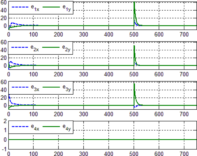
Graphic of the error coordinates of the robots

Figure 13.

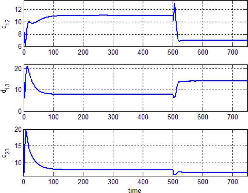
Distance between AGVs

The simulation shows three intervals of time where the three control laws (8)–(10) are implemented. The initial positions of the four robots are β₁ = (–10.5,0), β₂ = (–3.5,0),β₃ = (3.5,0) and β₄ = (10.5,0).

In Figure 12, for 0 ≤ t < 250, three robots are moved from their given home positions to the position of RM₁₂ in the triangle formation using the formation control law with collision avoidance (8). Note that the robots R₁,R₂,R₃ are chosen due to the minor distance with respect to the position of RM₁₂, and R₃ is selected as the leader. Note that the formation errors defined by e_i = α_i − α*₁, i = 1, …,4 converge to zero, where e _ix and e _iy refer to the error of robot i on the x and y axes, respectively. The position and orientation of the robots in the time instants t = 15s and t = 250s are depicted in Figure 11.

For 250 ≤ t ≤ 500, the formed robots apply the marching control law (10), where the marching path is given by the parametric equations for a straight line that begins in the position of RM₁₂ and ends in the position of PM₁. Note in Figure 12 that the error coordinates remains at zero, i.e., the formation is rigid during the path following. Figure 11 shows the marching of the robots in the time instants t = 375s and t = 500s .

Finally, in Figure 12, for 500 < t ≤ 750, the robots have finished the transportation of the workpiece and they use the control law (9), breaking formation to return to their home positions, avoiding again inter-robot collision. The coordination errors also converge to zero. Figure 11 shows the posture of the robots in the time instants t = 505s and t = 511s, very close of the home positions.

Figure 13 shows that during the three time intervals the variables d_ij, which denote the distance between robots R_i and R_j, are greater than the diameter d, i.e., the robots do not collide. The time interval 250 ≤ t ≤ 500 shows that the distance between robots satisfies the proposed pattern formation. Finally, in 500 < t ≤ 750 the robots eventually break the formation and return to home. Note that robot 4 remains at home because it is not used by the task. On the other hand, if the robots have finished the transportation of a piece, they can be assigned to another task instead of implementing control law (9) and returning to their home position.

Remark 2. Note that the coordination of the AGVs in the approach is composed of two levels. In the higher level, the PN model enables the transportation tasks considering the availability of the robots and the restrictions of the process. The AGVs are selected according to the shortest distance to the initial point of the task. The PN model has the capacity to execute concurrently different transportation tasks, as shown in the example in the next section. On the other hand, every task in low-level control implements continuous control laws for the robots to achieve the desired motion behaviour. Therefore, the hybrid architecture solves the problems of task assignment and convergence to a formation, tracking and collision avoidance at the same time.

6. Case study

Figure 14 shows the FMS including a set of r = 4 AGVs, two PM (PM₁ and PM₂) and two AS (AS₁,AS₂). PM₁ performs k₁ = 2 machining programs M₁₁,M₁₂ and PM₂ performs k₂ = 1 machining program M₂₁. Thus, the raw material storage locations are RM₁₁, RM₁₂ or RM₂₁.

Figure 14.

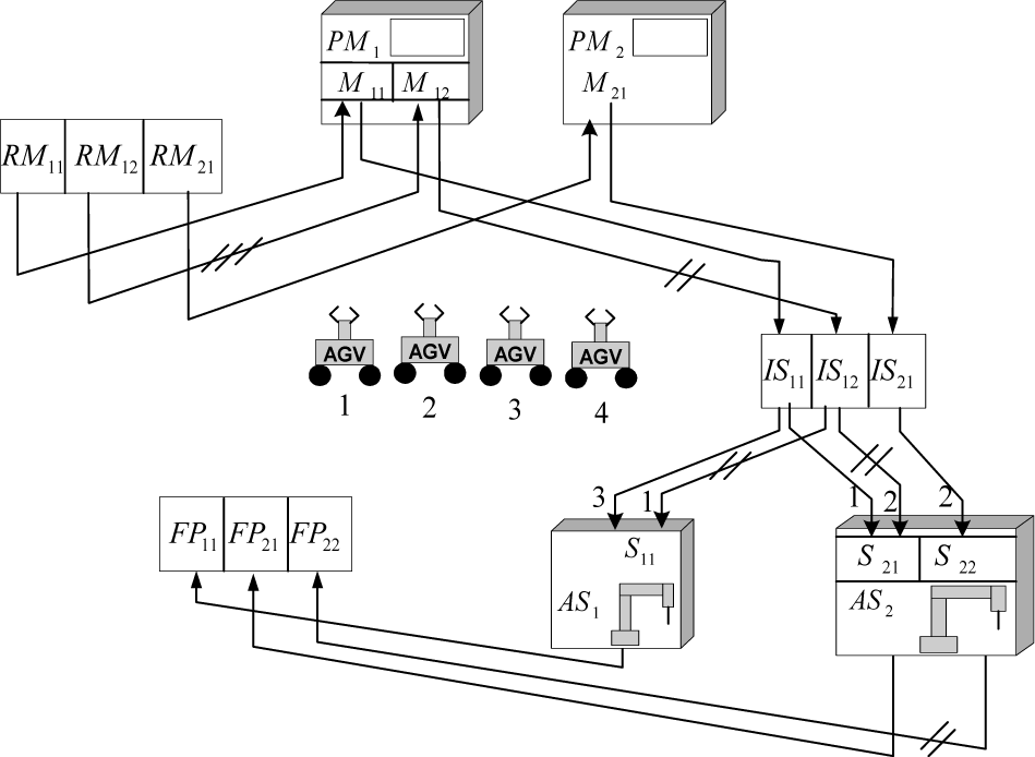
Scheme of the elements and tasks of an FMS

For the transportation of the raw material RM₁₂ to PM₁, it is necessary that n₁₂ = 3 AGVs (denoted by little crossed lines). Note that in the scheme of Figure 14, RM₁₁ and RM₂₁ only require one AGV (by default omitting the line cross). The AGVs move the machined parts to intermediate storage at IS₁₂ or IS₂₁. Observe that two AGVs m₁₂ = 2 are needed to move the parts from PM₁ to IS₁₂.

For the case of the assembly stations, AS₁ performs r₁ = 1 assembly program S₁₁ and AS₂ performs r₂ = 2 assembly programs S₂₁,S₂₂. The necessary subparts to achieve the products are defined by U(S₁₁) = {IS₁₁,IS₁₂}, U(S₂₁) = {IS₁₁,IS₁₂} and U(S₂₂) = {IS₂₁} in the quantities given by K(S₁₁, IS₁₁) = 3, K(S₁₁, IS₁₂) = 1, K(S₂₁, IS₁₁) = 1, K(S₂₁,IS₁₂) = 2 and K(S₂₂,IS₂₁) = 2. Note that two AGVs are required to move pieces from IS₁₂ to AS₁ or AS₂.

The final product storage locations are FP₁₁, FP₂₁, requiring one AGV; FP₂₂ requires two AGVs for transportation. The RM, IS and FP storage locations have capacity C(RM_ij) = 4, C(IS_ij) = 5 and C(FP_pq) = 3, respectively.

According to the general model of logical precedences, Figure 15 shows the diagram of this case study. Using the models presented in section 4, the PN of the FMS is shown in Figure 16.

Figure 15.

Diagram of precedences of the FMS

Figure 16.

PN model of the FMS case study

Remark 3. Note that the PN approach represents the concurrence that appears in an FMS in a more compact form than another planners like the automata approach. However, for a large FMS the PN model becomes less compact, especially if there exist many restrictions in the process. Despite this, it is possible to identify the generic blocks described in section 4.2, which construct the complete net. Therefore, the final PN model is a systematic method to achieve complex models based on simple blocks. On the other hand, the graphic representation of the PN model serves only as a visual tool in the process flow. In a real implementation, the control implementation will be realized using the mathematical structure instead of the graphical interpretation. Thus, the modelling approach based on generic blocks facilitates the translation to real supervisory control systems using the simple rules of the simple PN approach. In this sense, other PN formalism, like coloured PN, fuzzy PN, and others could complicate the codification of the PN and the definition of more properties of the generic blocks described in section 4.2.

Using a simulator of the PN dynamics, a phase-space diagram of the tasks of AGVs, PM and AS is given in the Figure 17. Note that the transportation tasks A₁, A₂, A₃ and A₄ of AGVs include the quantity of AGVs in each task.

Figure 17.

Phase-space diagram of distribution of AGV in concurrent tasks

To show the task distribution of the AGVs in the FMS, observe that the four robots are occupied in different routes, with task concurrency and distribution of the AGVs at the time instant t_α (see Figure 17).

7. Conclusions

This paper has presented a methodology for the discrete-event modelling of FMS based on the task decomposition proposed by the industrial standard ISA-95 and its translation to generic PN models. Interconnected equipment, storage locations, process tasks and inter-task logical precedences comprise a general PN model that describes the maximal concurrency obeying the process restrictions. The modelling approach allows the modification of the amount of equipment or storage limitations without necessitating changes to the network topology, preserving its static properties. The task-based modelling also provides a clear separation between the generic process tasks related to the equipment capacities and their interconnections for the manufacturing of different and concurrent products. The PN model provides the dynamical structure for a high-level supervision of the FMS in a control computer and the vigilance of the availability of equipment. The coordination of the AGVs is achieved by the implementation of formation, collision avoidance and marching control laws where the robots collaborate in concurrent transportation tasks. The approach adopts a systematic method that uses the concepts of discrete-event systems in an engineering manufacturing context, and clarifies the application of continuous motion control laws of AGVs in FMS.

8. Acknowledgements

This work was partially supported by the Universidad Iberoamericana, CONACyT (SNI scholarship) and IPN through research project 20140659 and scholarships EDI, COFAA, and PIFI.