A Dynamic Balancing Approach for a Quadruped Robot Supported by Diagonal Legs

Abstract

For legged robots, the most important task is to keep balance. This paper proposes a new balance control approach. To simplify the control complexity, first, LQR (linear quadratic regulator) control was used to obtain stable state feedback for the model. Then, the 6-DOF model was stabilized by dividing the whole robot into three separate parts. After that, VMC (virtual model control) was used to change the configuration of the joints. The simulation results showed that the proposed method allowed the quadruped robot to walk stably, even when certain types of disturbance were exerted on the models. In the simulation model, to mimic real conditions, noise was added to the sensors; the algorithm was then verified as still suitable for the quadruped robot.

1. Introduction

For legged robots, a robust balancing algorithm is needed to ensure stability. There are many methods for evaluating the stability margin required to keep a legged robot stable. The most commonly used criterion is the static stability criterion [1], which was proposed by McGhee and Frank in 1968. This method states that the vertical projection of the COG (centre of gravity) on the supporting plane must be within the support polygon enclosed by the supporting legs, and that the shortest distance between the projection and the edge of the support polygon can be defined as the SSM (static stability margin). In addition, Papadopoulos [2] has proposed force-angle stability, which included the effect of outer forces exerted on the robot, while Vukobratovic [3] proposed the concept of the ZMP (zero-moment point): a method that considers the effect of inertia force, giving a criterion that is widely used in biped robots. Much work has been done on the control of quadruped robots [4–13]. However, the control approaches and criteria mentioned above can only be used when the robot possesses a support polygon, formed either by several supporting legs or by large feet; thus, larger distances between legs and larger feet are often preferred so as to obtain a larger stability margin. When a robot's feet are too small or when the robot jumps into the air, these criteria can no longer be used.

In the 1980s, Raibert [14] proposed the foot placement algorithm (FPA) for the control of legged robots, which divided the balancing control of the robot into three elements: speed control, posture control, and hopping height control. This approach differed greatly from the static stable methods mentioned above. With this FPA method, a series of robots with one, two and four legs were developed [15, 16]. They were well balanced with small feet and few supporting legs, but they had to keep jumping all the time to prevent from falling, which can lead to an increase in the energy consumption of quadruped robots. Emura and Arakawa [17] built a reaction-wheel-type inverted pendulum to keep their quadruped robot stable. As a result, the quadruped robot could stand stably on two diagonal legs, but its balance was only held for about 10 seconds.

In this paper, a robust and effective method for balancing a quadruped robot using two diagonal supporting legs is proposed and the simulation results show the effectiveness of the proposed method.

The remainder of the paper is organized as follows: Section 2 describes the biped model approach, and the LQR control used to stabilize this system; in Section 3, the model is modified to include six DOFs; in Section 4, the direction of the coordinate system is changed and the model extended to match the most commonly used joint configuration; white noise is added to the ideal sensors in Section 5; and conclusions are given in Section 6.

2. The Balancing Control Strategy of the Simplest Biped Supporting Model

There are various quadruped robot prototypes, many of them using prismatic legs, such as Raibert's quadruped robot and the Scout II robot.

Figure 1.

Raibert's quadruped robot [16]

The legs of the robots are designed based on spring-loaded inverted pendulums and can run very fast. They can keep balance easily when running or standing with four legs, but they can hardly remain stable on two legs. This problem is discussed in this paper.

When a quadruped robot stands on its diagonal legs, the other two legs are drawn back to the body, and can be seen as part of the body, meaning the quadruped robot can be simplified in terms of a body and two diagonal legs. Therefore, to analyse the stability of a quadruped with two diagonal legs, the simplest biped supporting model should firstly be built.

Figure 2.

Scout II robot

In this model, two cylindrical legs are connected to a cuboid-shaped trunk by two rotary joints; the two legs stand on the ground. First, we will build the coordinate system of the model and deduce the Lagrange dynamics equation.

2.1 Coordinate Systems

All the bodies in the system are assumed to be rigid and the frame Σ _b is fixed in the trunk as shown in Figure 3. For convenience, the origin of Σ _b is set to the COG of the trunk. The front leg coordinate Σ _F is fixed in the front leg: the origin is fixed in the hip of this leg, the X axis points to the toe, and the Z axis points to the hind leg. Meanwhile, the hind leg coordinate Σ _H is fixed in the hind leg: the origin is also fixed in the leg hip, the X axis points to the toe of the hind leg, the Z axis shares the same direction as that of Σ _F , and the legs rotate around their Z axes.

Figure 3.

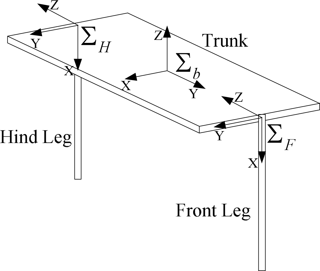
Coordinate systems of the biped robot model

2.2 Dynamics of the Biped Supporting Model

It is always important to analyse the dynamics of a particular robot, and there are many methods that can achieve this effectively [18–21]. In this paper, the Lagrange method is used to analyse the dynamics of the models.

Suppose the pitch angle θ _body , and the leg positions θ _FS and θ _HS , can be obtained by means of the attitude sensor and angle sensors. In this case, the two angles are defined as follows:

${\theta }_F={\theta }_{FS}-{\theta }_{body}$

(1)

${\theta }_H={\theta }_{HS}-{\theta }_{body}$

(2)

where θ _F is the angle between the front leg and the direction of gravity, and θ _H is the angle between the hind leg and the direction of gravity. The relationship between these angles is shown in Figure 4.

Figure 4.

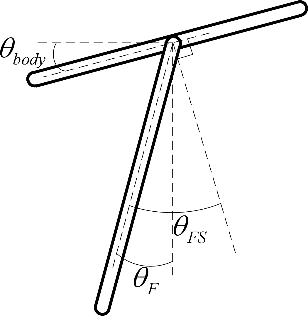
Angles of the biped model (front view)

In order to deduce the Lagrange equation of the model, the parameters of the symbols used are shown in Table 1 and these parameters are illustrated in Figure 5.

Table 1.

Parameters and values of the symbols

Symbol	Parameter	Value	Unit
m body	trunk mass	100	kg
m leg	mass of a single leg	5	kg
W	half of the trunk width	0.25	m
D	distance between the hips of the legs	1	m
L leg	length of each leg	0.5	m
g	gravity acceleration	9.8	m/s2
τ F	torque exerted by front hip actuator	Variable	Nm
τ H	torque exerted by hind hip actuator	Variable	Nm

Figure 5.

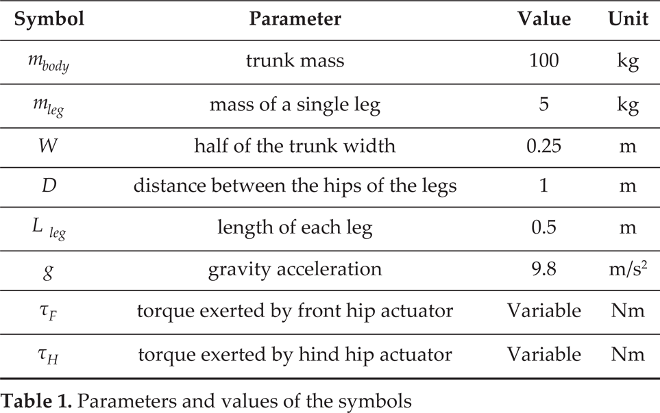
Illustration of the parameters (front view)

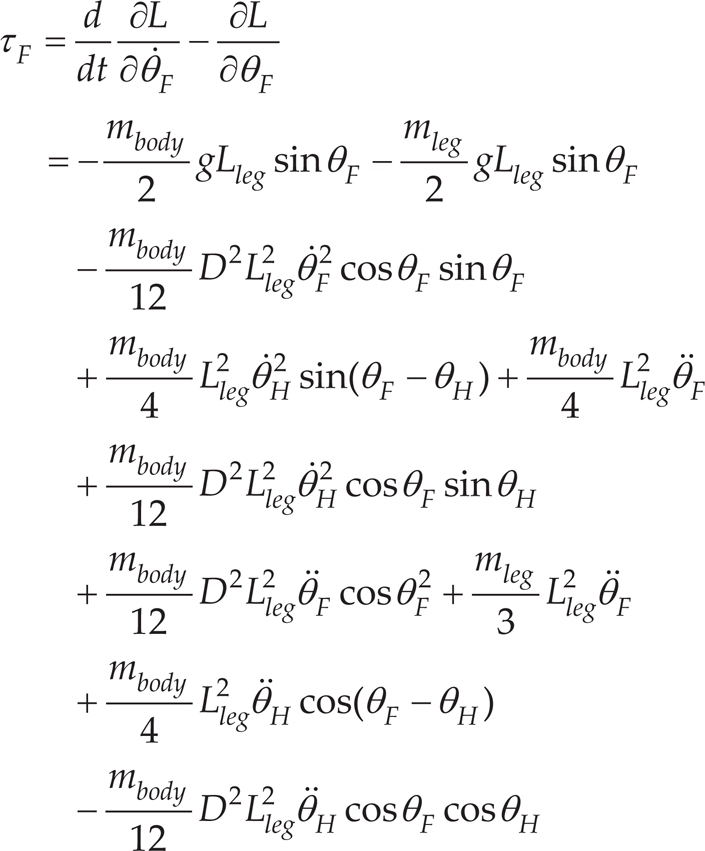
Based on the symbol definition above, the dynamic model of the biped supporting model can be derived from a Lagrange equation:

$\frac{d}{dt}\frac{\partial L}{\partial \dot{q}}-\frac{\partial L}{\partial q}=S\tau$

(3)

$L=\mathrm{\Sigma }{E}_k-\mathrm{\Sigma }{E}_p$

(4)

where E _k is the total kinetic energy, E _p is the total potential energy, $q={\left[{\theta }_F{\theta }_H{\theta }_{body}\right]}^T$ , $S={\left[\begin{array}{l}10-1\\ 01-1\end{array}\right]}^T$ and $\tau =\left[\begin{array}{c}{\tau }_F\\ {\tau }_H\end{array}\right]$

Additionally,

$\begin{array}{l}{\tau }_F=\frac{d}{dt}\frac{\partial L}{\partial {\dot{\theta }}_F}-\frac{\partial L}{\partial {\theta }_F}\\ =-\frac{m_{body}}{2}g{L}_{leg}\sin {\theta }_F-\frac{m_{leg}}{2}g{L}_{leg}\sin {\theta }_F\\ -\frac{m_{body}}{12}{D}^2{L}_{leg}^2{\dot{\theta }}_F^2\cos {\theta }_F\sin {\theta }_F\\ +\frac{m_{body}}{4}{L}_{leg}^2{\dot{\theta }}_H^2\sin ({\theta }_F-{\theta }_H)+\frac{m_{body}}{4}{L}_{leg}^2{\ddot{\theta }}_F\\ +\frac{m_{body}}{12}{D}^2{L}_{leg}^2{\dot{\theta }}_H^2\cos {\theta }_F\sin {\theta }_H\\ +\frac{m_{body}}{12}{D}^2{L}_{leg}^2{\ddot{\theta }}_F\cos {\theta }_F^2+\frac{m_{leg}}{3}{L}_{leg}^2{\ddot{\theta }}_F\\ +\frac{m_{body}}{4}{L}_{leg}^2{\ddot{\theta }}_H\cos ({\theta }_F-{\theta }_H)\\ -\frac{m_{body}}{12}{D}^2{L}_{leg}^2{\ddot{\theta }}_H\cos {\theta }_F\cos {\theta }_H\end{array}$

(5)

$\begin{array}{l}{\tau }_H=\frac{d}{dt}\frac{\partial L}{\partial {\dot{\theta }}_H}-\frac{\partial L}{\partial {\theta }_H}\\ =-\frac{m_{body}}{2}g{L}_{leg}\sin {\theta }_H-\frac{m_{leg}}{2}g{L}_{leg}\sin {\theta }_H\\ +\frac{m_{body}}{12}{D}^2{L}_{leg}^2{\dot{\theta }}_F^2\cos {\theta }_H\sin {\theta }_F\\ -\frac{m_{body}}{4}{L}_{leg}^2{\dot{\theta }}_F^2\sin ({\theta }_F-{\theta }_H)+\frac{m_{body}}{4}{L}_{leg}^2{\ddot{\theta }}_H\\ -\frac{m_{body}}{12}{D}^2{L}_{leg}^2{\dot{\theta }}_H^2\cos {\theta }_H\sin {\theta }_H\\ +\frac{m_{body}}{4}{L}_{leg}^2{\ddot{\theta }}_F\cos ({\theta }_F-{\theta }_H)\\ -\frac{m_{body}}{12}{D}^2{L}_{leg}^2{\ddot{\theta }}_F\cos {\theta }_F\cos {\theta }_H\\ +\frac{m_{body}}{12}{D}^2{L}_{leg}^2{\ddot{\theta }}_H{\cos }^2{\theta }_H+\frac{m_{leg}}{3}{L}_{leg}^2{\ddot{\theta }}_H\end{array}$

(6)

$\begin{array}{l}{\tau }_{body}=\frac{d}{dt}\frac{\partial L}{\partial {\dot{\theta }}_{body}}-\frac{\partial L}{\partial {\theta }_{body}}\\ =W^2{m}_{body}{\ddot{\theta }}_{body}\\ =-{\tau }_F-{\tau }_H\end{array}$

(7)

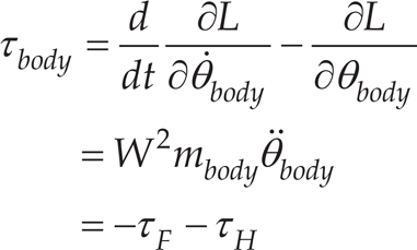
To control the balance of the biped supporting model, the state space equation of the model is constructed based on the following definition of the state variable: X=[θ _F θ _F θ _H θ _H θ _body θ _body ] ^T . Then, the dynamic equation is linearized and the state space equation can be defined as

$\dot{X}=AX+B\tau$

(8)

and a state feedback based on LQR control can be obtained to stabilize the system:

$\tau =-KX$

(9)

The control structure of the system is shown in Figure 6.

Figure 6.

Control structure of the system with state feedback

Since a too large hip torque may cause the slippage of the legs, the torque must be constrained. The maximum torque is determined by the maximum static friction force between the toe and the ground, and is shown as follows:

${\tau }_{\max }=\frac{{\mu }_{static}F}{L_{leg}}$

(10)

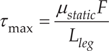
where μ _static is the coefficient of static friction, and F is the normal force that the leg exerts on the ground. If the expected hip torque exceeds τ_max, it is limited to τ_max.

3. Balance of a 6-DOF Diagonal Leg Model

In the biped model, each leg is constrained in a single plane. Hence, to allow the legs to work in 3D space, a 6-DOF model must be built. In this model, each leg has three active DOFs: the joint nearest to the hip rotates around the trunk diagonal line, the next joint rotates around the axis that is perpendicular to the diagonal line in the trunk plane, and the third joint is a prismatic joint that moves along the leg and can change the length of the leg. Based on this type of joint configuration, the motion can be decoupled into three parts, with each pair of legs resisting one type of disturbance. The decoupling mechanism is shown in Figure 7.

Just as the motion of the 6-DOF model is divided into three parts, so the control of the whole robot is also divided into three parts. As is shown in Figure 7, Part A controls the torques of the two joints around the diagonal line against postural disturbance, Part B controls the torques of the other two hip joints to resist disturbance along the diagonal line, and Part C controls the forces of the two prismatic joints to maintain the height of the robot. Of the three decoupled models, Part B and Part C are easily controlled by a PID controller, since they do not contain any dynamically balancing problems.

Therefore, the only problem is how to balance Part A to maintain the walking stability of the robot. The model of Part A is similar to the biped supporting model, so a similar control method can be applied to this part. However, before LQR control can be used, some modifications should be made. The coordinate systems of this model are different, as shown in Figure 8.

Figure 7.

Joint configuration of the 6-DOF model and the decoupled models

Figure 8.

Coordinate systems of Part A

In Part A, the body rotation is around the diagonal line of the trunk, meaning the traditional Z-Y-X Euler angles cannot be used for body rotation angle feedback directly and a transformation is therefore needed. Here, Z-Y-K angles are built, as shown in Figure 9; these are similar to Z-Y-X Euler angles, but the third rotation is not around the X axis of the moving coordinate system. Instead it rotates around the K axis, which is in the same direction as the diagonal line determined by the hips of the two supporting legs.

Figure 9.

Rotation representation of Z-Y-K angles for the 6-DOF model

The transformation matrix can be defined as follows:

$\begin{array}{l}{R}_{zyk}=R_z({\theta }_z)R_y({\theta }_y)R_k({\theta }_k)\\ =\left[\begin{array}{ccc}{R}_{11}& R_{12}& R_{13}\\ R_{21}& R_{22}& R_{23}\\ R_{31}& R_{32}& R_{33}\end{array}\right]\end{array}$

(11)

where R _z (θ _z ) represents the rotation matrix around the Z axis of the rotating coordinate system, and the rotation angle is θ _z .

So

$\{\begin{array}{c}\sin {\theta }_y=\frac{B{R}_{32}-A{R}_{31}}{A}\\ \sin {\theta }_z=\frac{A^2{R}_{21}\cos {\theta }_y-AB{R}_{22}\cos {\theta }_y-B^2{R}_{12}+AB{R}_{11}}{A^2{\cos }^2{\theta }_y+B^2}\\ \cos {\theta }_z=\frac{A^2{R}_{11}\cos {\theta }_y-AB{R}_{12}\cos {\theta }_y+B^2{R}_{22}-AB{R}_{21}}{A^2{\cos }^2{\theta }_y+B^2}\\ \sin {\theta }_k=\frac{B{R}_{31}\cos {\theta }_y+B{R}_{33}\sin {\theta }_y+A{R}_{32}\cos {\theta }_y}{B^2{\sin }^{2}y+{\cos }^{2}y}\\ \cos {\theta }_k=\frac{R_{33}\cos {\theta }_y-B^2{R}_{31}\sin {\theta }_y-AB{R}_{32}\sin {\theta }_y}{B^2{\sin }^{2}y+{\cos }^{2}y}\end{array}$

(12)

where

$A=\frac{D}{\sqrt{D^2+W^2}}$

(13)

$B=\frac{W}{\sqrt{D^2+W^2}}$

(14)

In this model, the state variable θ _body is set to θ _k , which is still the rotation angle of the trunk. Since the only changes are the positions of the hips of the legs, the behaviour of the closed-loop system is the same as in the previous biped model.

4. Balance of the Diagonal Legs Model

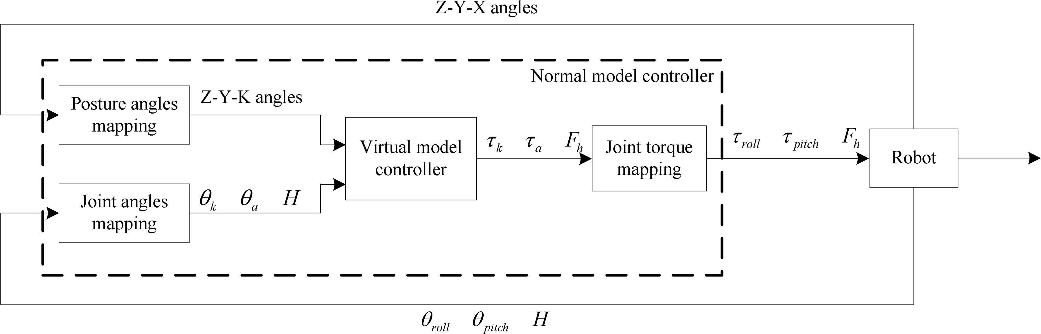
In the previous section, the joints rotated around or were perpendicular to the diagonal line, but this structure is seldom used in the real world. For most quadruped robots, the legs are composed of roll joints and pitch joints, so further modifications are needed. Here, virtual model control (VMC) [22] is used as a bridge between the diagonal joints model and the common joint configuration model of quadruped robots, as shown in Figure 10.

The procedure of using the virtual model can be divided into three steps: firstly, mapping the sensor information from the normal model onto the virtual model; then, using the controller of the virtual model to calculate the output virtual torque that should be exerted on the virtual model; and finally, mapping the control force and torque of the virtual model onto the normal model. The transformation between the virtual model controller and normal model controller is illustrated in Figure 11.

Figure 10.

Change of the direction of the joints

Figure 11.

Transformation between the virtual model controller and the normal model controller

Based on the method of virtual model control, kinematic equations of the two models can be obtained. As the length of the leg is almost a constant, H is used as an approximate value to simplify the equations. Equation 15 shows the direct kinematic equation of the virtual model, and equation 16 shows that of the normal model.

$\begin{array}{l}\left[\begin{array}{c}x\\ y\\ z\end{array}\right]={}_{}{}^{G}R{}_0{}_{}{}^{0}R{}_K{}_{}{}^{K}R{}_A\left[\begin{array}{c}H\\ 0\\ 0\end{array}\right]\\ =\left[\begin{array}{c}\frac{D\sin {\theta }_a+W\cos {\theta }_a\sin {\theta }_k}{\sqrt{D^2+W^2}}H\\ \frac{D\cos {\theta }_a\sin {\theta }_k-W\sin {\theta }_a}{\sqrt{D^2+W^2}}H\\ -\cos {\theta }_k\cos {\theta }_{a}H\end{array}\right]\end{array}$

(15)

$\left[\begin{array}{c}x\\ y\\ z\end{array}\right]=\left[\begin{array}{c}\sin {\theta }_{roll}\\ \sin {\theta }_{roll}\cos {\theta }_{pitch}\\ -\cos {\theta }_{roll}\cos {\theta }_{pitch}\end{array}\right]H$

(16)

Therefore, the joint angles of the normal model can be mapped to the virtual model, based on the above two equations:

${\theta }_k={\tan }^{-1}\frac{W\frac{\tan {\theta }_{pitch}}{\cos {\theta }_{roll}}+D\tan {\theta }_{roll}}{\sqrt{D^2+W^2}}$

(17)

${\theta }_a={\sin }^{-1}\frac{D\sin {\theta }_{pitch}-W\cos {\theta }_{pitch}\sin {\theta }_{roll}}{\sqrt{D^2+W^2}}$

(18)

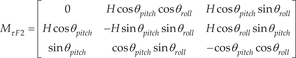
The force Jacobians can be derived from kinematic equations. In the virtual model, the force Jacobians are defined as

$\left[\begin{array}{c}{\tau }_k\\ {\tau }_a\\ F_h\end{array}\right]=M_{\tau F1}\left[\begin{array}{c}{F}_x\\ F_y\\ F_z\end{array}\right]$

(19)

and in the normal model of quadruped robot, they are

$\left[\begin{array}{c}{\tau }_{roll}\\ {\tau }_{pitch}\\ F_h\end{array}\right]=M_{\tau F2}\left[\begin{array}{c}{F}_x\\ F_y\\ F_z\end{array}\right]$

(20)

Hence, the relationship between the torques of the two models can be obtained from equation 19 and equation 20:

$\left[\begin{array}{c}{\tau }_{roll}\\ {\tau }_{pitch}\\ F_h\end{array}\right]=M_{\tau F1}{M}_{\tau F2}{}^{-1}\left[\begin{array}{c}{\tau }_k\\ {\tau }_a\\ F_h\end{array}\right]$

(21)

where

$M_{\tau F1}=\left[\begin{array}{ccc}\frac{W\cos {\theta }_a\cos {\theta }_k}{\sqrt{D^2+W^2}}H& \frac{D\cos {\theta }_a\cos {\theta }_k}{\sqrt{D^2+W^2}}H& H\cos {\theta }_a\sin {\theta }_k\\ \frac{(D\cos {\theta }_a-W\sin {\theta }_a\sin {\theta }_k)}{\sqrt{D^2+W^2}}H& \frac{(-W\cos {\theta }_a-D\sin {\theta }_a\sin {\theta }_k)}{\sqrt{D^2+W^2}}H& H\cos {\theta }_k\sin {\theta }_a\\ \frac{D\sin {\theta }_a+W\cos {\theta }_a\sin {\theta }_k}{\sqrt{D^2+W^2}}& \frac{-W\sin {\theta }_a+D\cos {\theta }_a\sin {\theta }_k}{\sqrt{D^2+W^2}}& -\cos {\theta }_a\cos {\theta }_k\end{array}\right]$

(22)

$M_{\tau F2}=\left[\begin{array}{ccc}0& H\cos {\theta }_{pitch}\cos {\theta }_{roll}& H\cos {\theta }_{pitch}\sin {\theta }_{roll}\\ H\cos {\theta }_{pitch}& -H\sin {\theta }_{pitch}\sin {\theta }_{roll}& H\cos {\theta }_{roll}\sin {\theta }_{pitch}\\ \sin {\theta }_{pitch}& \cos {\theta }_{pitch}\sin {\theta }_{roll}& -\cos {\theta }_{pitch}\cos {\theta }_{roll}\end{array}\right]$

(23)

5. Simulation and Analysis

5.1 Simulation of the Biped Robot

The control method was tested in RobotBuilder [23], a simulation software based on the DynaMechs [24] dynamics engine. The environment parameters were set according to Table 2.

Table 2.

Environment parameters

Ground normal spring stiffness (N/m)	100000
Ground planar spring stiffness (N/m)	10000
Ground normal damper (Ns/m)	3000
Ground planar damper (Ns/m)	1000
Coefficient of static friction	0.4
Coefficient of kinetic friction	0.3

In the simulation, the closed-loop system was able to maintain balance for a long time; therefore, to test the stability of the biped model, various disturbances were exerted on the robot model. The pitch angular velocity was set to 1rad/s, 2rad/s, and 3rad/s, consecutively. The results of the simulation showed that the robot did not lose balance, and the three angles converged towards zero slowly, as shown in Figure 12.

Furthermore, yaw angular velocity was added to the system to test its torsional stability; the four disturbances were 1rad/s, 2rad/s, 3rad/s, and 4rad/s, separately. From Figure 13, we can see that the robot didn't fall down but that the legs moved on the ground. During the motion, the hip torque constraints were still effective; the slippage was instead caused by the fast rotating trunk, which pulled the legs up from the ground for a very short time. When the legs touched the ground again, the trunk began to slow down and finally all the state variables returned to zero.

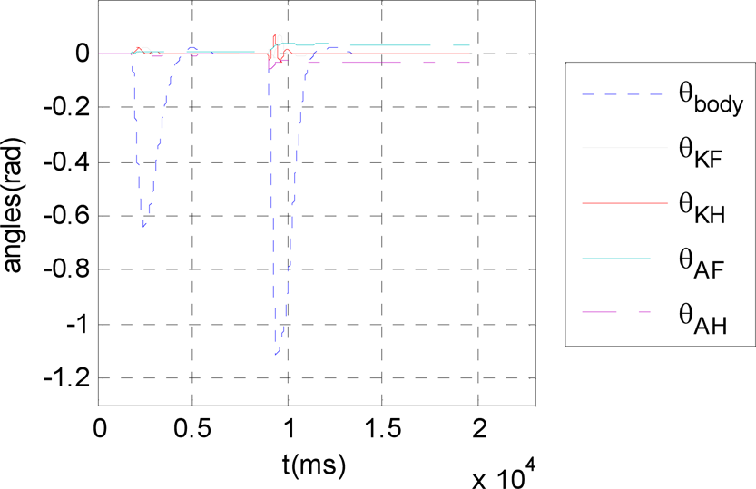
The previous disturbances to the robot model were all symmetrical disturbances, which did not affect the position of its COM (centre of mass). Lateral disturbance was harder to resist, since the legs were not allowed to move on the ground; in this case, a little displacement can cause large gravitational moment, causing the robot to fall to the side. Here, however, the method showed great robustness. A lateral velocity disturbance of 0.1m/s was imposed on the trunk, but the biped robot did not fall to the side. Instead, the trunk suddenly changed its posture to nearly vertical, which caused the COM to move to the opposite position, and then slowly move back to the equilibrium position. The trajectories of these variables are shown in Figure 14.

Figure 12.

Pitch angle disturbance test of the biped robot

Figure 13.

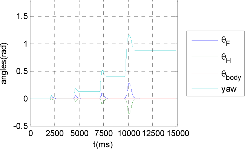
Yaw angle disturbance test of the biped robot

Figure 14.

Lateral velocity disturbance test of the biped robot

5.2 Simulation of the 6-DOF Model

In this section, postural disturbance was tested. The angular velocity was set to 1rad/s and 2rad/s. Although the robot remained stable, its ability to resist disturbance seemed weaker than that of the 2-DOF biped model, and the final values of the angles did not return to exactly zero. This was because, in this case, the disturbance's angular velocity rotated around the X axis of the body rather than the diagonal line. The initial angular velocity was so large that the front leg lifted off the ground for a short time, and the touch-down point was a little further out, meaning that θ _AF and θ _AH drifted from zero. Curves of the logged data are shown in Figure 15.

Figure 15.

6-DOF model with roll angular velocity disturbance

Figure 16.

6-DOF model with yaw angular velocity disturbance

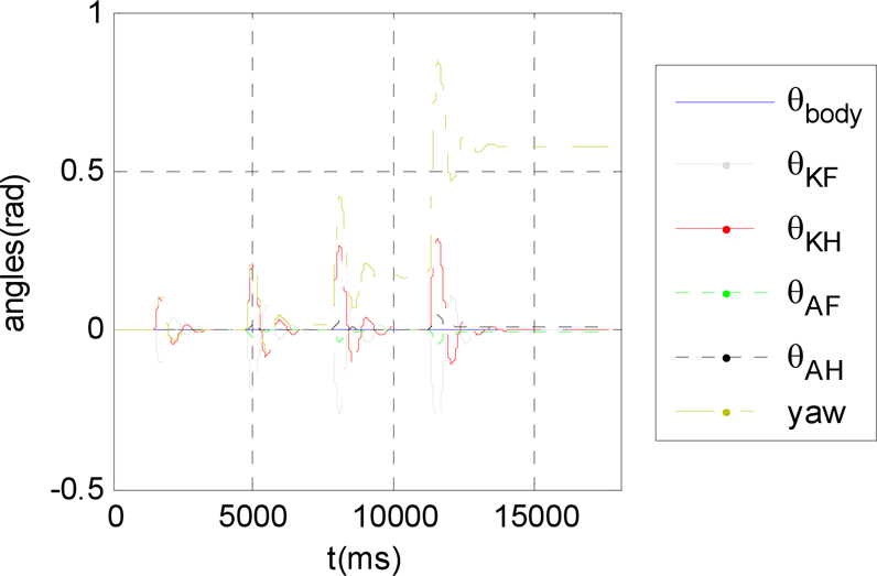
Yaw angular velocity disturbance was tested on the 6-DOF model (Figure 16). The angular velocities were set to 1rad/s, 2rad/s, 3rad/s, and 4rad/s, which were the same as for the 2-DOF biped model. Although it had more degrees of freedom, the robot was still able to remain stable when disturbed. Slippage also occurred, but the final yaw angle was not as large as it was for the 2-DOF biped model. This was because the lengths of the legs were variable; therefore, when the legs lifted off the ground, they extended a little, and this had the advantage of stopping the torsional motion.

The model's resistance to lateral velocity disturbances was also better than that of the 2-DOF biped robot (Figure 17), when lateral velocities of 0.1m/s and 0.2m/s were tested. This is because the lateral velocity disturbance could be seen as having two parts. One part was along the diagonal line, which was easily resisted by the active joints; the other part was perpendicular to the diagonal line, and this part could be stabilized only by adjusting the posture of the body, just like the lateral velocity disturbance in the 2-DOF biped model.

Figure 17.

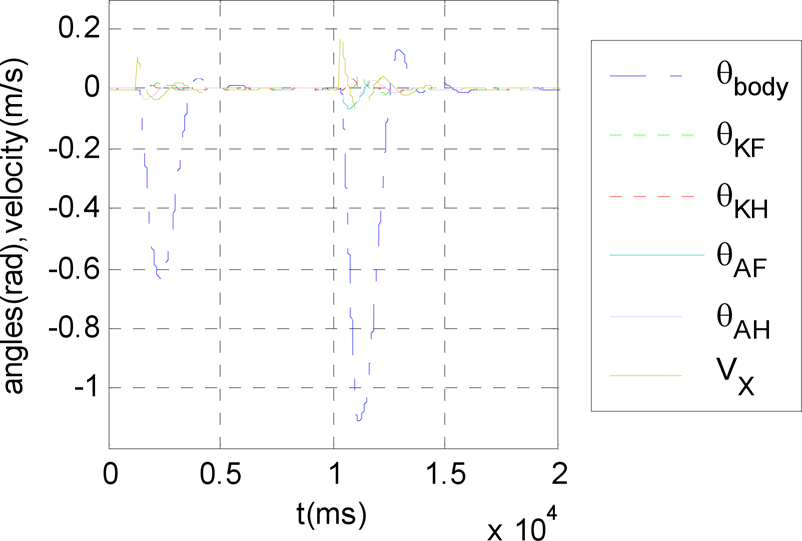
6-DOF model with lateral velocity disturbance

5.3 Simulation of the Normal Model

The three kinds of disturbances were also tested on the normal model, and the angles of the joints were logged. The results are shown in the figures below. In Figure 18, the roll angular velocity was set to 1 rad/s and 2 rad/s respectively; the maximum roll angles, the time taken to return to horizontal for the first time, and the duration of the overshoot were all similar to the virtual model. Figure 19 shows the data when yaw velocity disturbances of 1rad/s, 2rad/s, 3rad/s and 4rad/s were exerted on the model, and Figure 20 shows the model's behaviour after lateral velocities of 0.1m/s and 0.2m/s were applied. The data from the normal model were always similar to those of the virtual model.

Figure 18.

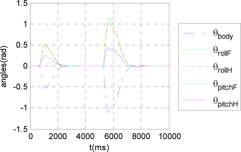
Trunk roll angular motion in the normal model

Figure 19.

Trunk yaw angular motion in the normal model

Figure 20.

Trunk lateral velocity disturbance in the normal model

5.4 Simulation with Noise

In the real world, there is electromagnetic interference everywhere, so the signals from the sensors may be mixed with noise. To make the simulation more realistic, white noise was overlaid on the data from each ideal sensor, and the Box-Muller method was used to ensure the independence of the random numbers, which obeyed Gaussian distribution. The mean value of the noises was zero, the standard deviation of the joint angle sensors was set to 0.001rad, and the standard deviation of the posture angle was set to 0.005rad. This precision could be reached by sensors commonly used at present. A Kaiman filter was used to smoothen the raw data mixed with noise. Figure 21 shows the process of the adjustment after roll angular disturbance, in simulation; the posture of the robot and the coordinate axes of each joint were clearly shown in RobotBuilder. Figures 22 to 24 give the simulation results. The roll angular motion test and the lateral velocity test both showed the effect of the noise; the posture of the trunk could not return to horizontal but fluctuated a little, although the robot did not lose balance. The robustness of the system against yaw angular motion was weakened; only 1rad/s and 2rad/s disturbances were tested, and the latter nearly toppled the robot.

Figure 21.

Snapshots of the simulation under roll angular motion

Figure 22.

Trunk roll angular motion with noise

Figure 23.

Trunk yaw angular motion with noise

Figure 24.

Trunk lateral velocity disturbance with noise

6. Conclusions

Balance control is a very important consideration for legged robots; most of them maintain balance with a support polygon formed by large feet or more than three legs, or they are hopping robots that need to jump all the time to keep balance. In this paper, a novel method of balance control was proposed to stabilize the motion of a quadruped robot. The model uses just two diagonal legs to support the body, and each leg makes contact with the ground at only a single point, so neither a support polygon nor jump motion is involved. Several models had been built to resolve the above problem; these evolved step by step, before the diagonal leg supporting model was finally built. In the proposed method, LQR control was used to stabilize the systems. In order to control the model with six DOFs, control of the robot's whole body was separated into three independent parts, with each part stabilized by its own controller. VMC was used in the last model. Each model was tested under several types of disturbances in RobotBuilder, and the simulation results showed that they all had good stability; they were not only able to maintain their balance, but they also resisted these disturbances. In particular, these models showed great robustness against lateral velocity disturbances; the trunk would suddenly adjust its posture automatically to reduce lateral speed, and then return to a stable state. This method could also be applied to legged robots with other numbers of legs: biped robots could use the first model directly, and hexapod or octopod robots could also keep their balance using only two supporting legs.