Sage Journals: Discover world-class research

Abstract

This paper presents the design of a novel quadruped robot. The proposed design is characterized by a simple, modular design, and easy interfacing capabilities. The robot is built mostly from off-the-shelf components. The design includes four 3-DOF legs, the robot body and its electronics. The proposed robot is able to traverse rough terrain while carrying additional payloads. Such payloads can include both sensors and computational hardware. We present the robot design, the control system, and the forward and inverse kinematics of the robot, as well as experiments that are compared with simulation results.

Keywords

Quadruped Robot Robot Design Research Platform

1. Introduction

In many cases, there is a need for mobile platforms that can move in areas with difficult terrain conditions where wheeled vehicles cannot travel. Examples of such scenarios can be seen in search and rescue tasks, as well as in carrying payloads. Unlike wheeled robots, walking robots are characterized by very good mobility in rough terrain. The main goal of this paper is to present an innovative, modular and inexpensive design of a four-legged robot for locomotion research purposes.

Investigation of walking machines began in the 19th century. One of the first models appeared around the year 1870 [18]. For 80-90 years, efforts were made to build walking machines based on different kinematic chains that were supposed to generate a desired motion profile during operation. During those years, many models were proposed, but the performance of most of these machines was limited by regular cyclic walking forms and the inability to adjust a walking pattern to the terrain. In the late 1950s, it became clear that machines should not just be based on kinematic mechanisms that provide cyclic movements, and that there was a need to integrate planning and control systems. The first robot to move autonomously with computerized control and electric propulsion was built in 1966 by McGhee and Frank [19]. The main task of the robot's computer was to solve the kinematic equations involved and to control the electric motors that drove the legs, such that the robot could go forward while maintaining equilibrium constraints. Since then, and following the advance of control technique technologies, computing resources and motion actuators, many different robots with varied abilities have been built. Examples of these abilities include running [10], walking over rough terrain, jumping over obstacles [14], climbing [24, 25] and more.

Today, there are a large number of active research programmes in the field of legged locomotion [27, 1, 9, 8, 15, 4, 22, 11, 2]. Apart from designing and building the robot itself, the main challenges are the planning and implementation of the legs' motions in generate a walking sequence, namely, how to plan the steps of the robot so that it moves in a desirable way while maintaining equilibrium constraints (quasi-static walking) or else maintaining the stability of the robot (dynamic walking).

However, in all the above studies, a considerable amount of research effort has gone into the design of the robot. Our goal is to present a simple, open-source, legged robot platform that will allow researchers to spend more of their time and funding on motion planning and less on robot design and construction. At present, many research groups develop their own robots for the testing and verification of algorithms and theories [32, 7, 21, 13, 12, 23, 17]. In most cases, the main subject of the research is not the robot itself but the locomotion theories involved. Usually, these robots are built and controlled in a complex manner that makes it difficult for other researchers interested in working with a similar platform to easily reproduce a similar robot. In addition, these robots are usually not designed in a modular fashion that allows for the changing of their structure and geometry in a simple and fast manner. We present in this paper the design of a four-legged walking robot which is suitable for use as a research tool in the motion-planning of four-legged robots. The use of the design presented will allow researchers to focus on major research topics without wasting time and resources in developing research tools. A significant advantage of the presented design is its ability to reproduce the results of other research papers on four-legged robots locomotion. Therefore, our design can serve as a standardized platform in this field of research. The main advantages of the presented robotic platform are design simplicity, structure modularity, low cost and a simple interface.

Currently, there are number of lab-scale quadruped robots being used in research, such as LittleDog [32] from Boston Dynamics, StarlETH [7] and ALoF [21] from ETH, TITAN-IX [13], MRWALLSPECT III [12], the “spider-like robot” [23] developed at Technion, AiDIN-III [16] from Sungkyunkwan University (SKKU), and others. These models have complex mechanical designs, such as custom-made joints and structures, non-uniform motors and custom electronics. These models are specifically designed with powerful processing units or built-in sensors. The main advantage of the design presented in this paper is that it can be built from off-the-shelf products. Therefore, it can be used immediately in a simple and cost-effective manner. In addition, the proposed robot is based on open-source code and hardware, thus enabling future improvements. Such improvements might include sensor capabilities, control circles and the mechanical structure. The combination of the mentioned design features makes the robot unique and innovative and leaves it optimized for research purposes.

The paper is structured as follows: Section 2 describes the mechanical design of the robot. Section 3 describes the electronic design as well as the communication and control methods for the robot. Section 4 presents in detail the financial cost of the robot. Section 5 describes the development of the forward and inverse kinematics equations of the robot and presents the robot workspace. Section 6 presents experiments conducted to demonstrate and verify the design and kinematics computations presented in the previous sections. Finally, Section 7 concludes and discusses future work.

2. Quadruped Robot Design

The robot was specifically designed to be simple, modular and built from off-the-shelf components. Each of the four legs is composed of three electric motors, which results in a 3-DOF for each leg. The robot leg design is shown in Figure 1.

Figure 1.

Front (a), and Side (b) exploded views of the robot leg design

We used Dynamixel RX-64 servo motors [34]. The RX-64 Dynamixel robot servo actuator is one of Robotis' most powerful smart actuators. It can provide 64 kg*cm of torque (18V supply) and it can traverse its entire 300 $^{\circ}$ range in under one second. Each servo can send back to the control software its speed, temperature, shaft angle, voltage and load. The control algorithm used to maintain the shaft angle can be adjusted individually for each servo, allowing for the control of the speed and strength of the motor's response. With the use of the RX-64 actuators, load feedback can be used both for energy calculations and the analysis of phenomena occurring at the contact points of the robot feet with the ground, such as detecting the moment of contact with the ground. The use of the RX-64 motors allows the robot to carry a payload of about 2.5 kg. The calculation is done considering a worst case scenario when the robot's weight is supported by just two legs which are spread horizontally. This scenario arises when the robot is standing on three legs while almost all of its weight is supported by only two legs. Figure 2 illustrates this worst case scenario.

Figure 2.

An illustration for a worst case torque demanding posture

When using the dimensions from Table 1 for the presented robot configuration, we get the required motor torque, $T_{r e q u i r e d} = 3.5 [N m]$ . One RX-64 motor can provide $5.2 [N m]$ (15V supply) while RX-28, which is the lower level in the Dynamixel servo series, can provide only $3.67 [N m]$ (16V supply). This does not allow a large enough safety margin. Hence, we chose to use the RX-64 motors for all 12 joints for both convenience and modularity.

Table 1.

Design parameters' values

Sign	Description	Value
W	Body width	24.5 [cm]
H	Body height	22.5 [cm]
$l_{0}$	$l_{0}$ length	2 [cm]
$l_{1}$	$l_{1}$ Link length	4 [cm]
$l_{2}$	$l_{2}$ Link length	10.5 [cm]
$l_{3}$	$l_{3}$ Link length	10.5 [cm]
$θ_{1_L i m i t}$	$θ_{1}$ Actuator physical limit	150°
$θ_{2_L i m i t}$	$θ_{2}$ Actuator physical limit	112°
$θ_{3_L i m i t}$	$θ_{3}$ Actuator physical limit	112°
M	Robot weight (battery included)	3.4 [kg]

All the sensor management position control and serial RS-485 communication are handled by the servo's built-in microcontroller. This distributed approach leaves the main robot controller free to perform higher-level tasks. The motors are mechanically interconnected using standard aluminium links [31]. These links are replaceable off-the-shelf components. By using other types of link or different sized links, it is possible to change the dimensions of the robot legs and the configuration of the motors. In addition to considerations of minimal design and modularity, the selection of these links' configuration allows for a symmetric and sufficiently large workspace, as described later in this section. The legs end-links are standard M8×1.25×50 screws fastened with nuts. Various footpads can be connected at the end of these screws. These footpads serve as the leg contact points with the ground. In the presented design, the legs' footpads are made from round-ended plastic and rubber cylinders printed with a rapid, prototype 3D printer. The screws at the bottom of the legs can be replaced with a more complex link which includes springs and dampers in order to add desired physical characteristics to the robot legs.

The body of the robot consists of two parallel, 2 mm-thick, aluminium plates. The plates are connected to each other using four aluminium blocks with holes suitable for fixing the aluminium links in various ways. This allows a modular setup for the orientation of the upper degree of freedom of the legs. The bottom plate contain holes that are used to secure the battery and electronics inside the robot body. Figure 3 shows the structure of the robot and the robot's dimensions.

Figure 3.

Top fig:xy and side fig:xz views of the robot design. The figure presents the symbolic dimensions and locations of the coordinate frames.

In order to represent the robot configuration, we define a set of coordinate frames. Section 5 will discuss the use of these frames in developing the robot forward and inverse kinematics equations. Table 1 lists the dimensions and values of the design parameters. These dimensions allow the robot to reach a ground area with a 10 cm radius disc, while the body is horizontal and at 20 cm height above the ground. Furthermore, this configuration increases the omni-directionality of the robot's legs. This is a result of orienting the upper leg joints' axes perpendicular to the body plane. With this configuration, each robot leg can place its footpad on obstacles with a maximum height of 21 cm. However, in order to pass over such a high obstacle, it is necessary to carefully plan the trajectory of all the legs and the centre of mass in order to maintain stability.

This configuration of parameters allows us to assume that the centre of mass of the robot is relatively unaffected by the position of its legs (i.e., we can assume that the robot's legs are massless). This assumption greatly simplifies the calculations performed by the foothold planning algorithms that are required to calculate the position of the robot's centre of mass. The change of location of the centre of mass due to the legs' movement does not exceed the dimensions of a 2.2 cm radius sphere. The calculation for the above assertion was performed using SolidWorks¹ software. The robot was completely modelled and each part was assigned with its own mass. We used SolidWorks to calculate the location of the centre of mass while varying the joint angles of the robot legs. As expected, the extreme values were obtained when the robot legs were all spread out in the same direction. This information can be used by the motion planner to add adequately large stability margins which will ensure the robot's stability even when its legs are moving. It is important to note that the above assumption should only be made after the examination of the robot's configuration. Changes in the legs' links or in the robot's body weight require revisiting the massless legs assumption. Moreover, when the motion is not slow, we must consider the effect of the robot's mass and inertia for the analysis of dynamic effects.

3. Control and Communication

The robot's main controller is the ArbotiX robocontroller [30]. The ArbotiX robocontroller is a high-end AVR-based robot controller. It is specifically designed to control robots built using the Robotis Dynamixel servos. The ArbotiX is based on the ATMEGA644p microcontroller, offering 32 I/O ports, a XBee socket for wireless communication, a dual 1A motor driver, and more. The ArbotiX can be used with the Arduino IDE, which allows for a simple and convenient programming environment. The 12 RX-64 motors are connected to the ArbotiX through the RX Bridge [29], which communicates with the motors. The power source used to operate the controller and the motors is a 4S LiPo battery, but it can also be powered by a power supply connection. The LiPo battery voltage is monitored using the ArbotiX analogue input pins in order to prevent over-discharge. Wireless communication with the robot is based on the XBee 2.4 Ghz radio modules [35].

The robot software can be divided into two parts. The first part comprises the low-level motor control, while the second part comprises a high-level robot motion-planning algorithm. In the low level control, we use the BioloidController library [28] in order to create a smooth transition between two different robot positions. This library implements a low-level serial communications code for communication with the motors and the implementation of functions, which allows for the use of a single command to control all 12 motors in a coordinated manner. This command includes a 12 element vector indicating the goal position of each motor. The RX-64 motors are too fast to use without speed control and a velocity profile. Rapid motion can affect the robot's stability. Hence, we use an interpolation method to enable a gradual motion. The BioloidController library consists of an interpolation engine which allows this to be done while giving the user the option to set the total interpolation time. The interpolation engine plans the motion of all the motors such that they will move in a coordinated manner (i.e., start and complete the motion at the same time). The BioloidController library also allows us to receive the current motors' positions, speeds, loads and other parameters.

Although the control loop presented in this paper only refers to the position control of the robot motors, the necessary hardware and software capabilities allow for the further development of more sophisticated control methods, such as speed and torque control. The use of position control is mainly suitable for scenarios where the robot's motion is slow, such as climbing or walking on very rough terrain.

This high-level motion planning can include any existing or under-development motion-planning algorithm which outputs the required robot joint angles for each step. Such an algorithm can range from a pre-defined cyclic-gait to a highly complex gait generator that takes into account stability constraints and terrain geometry. The algorithm can be realized in any programming language which supports the establishment of a serial communication port. This serial port is connected to the XBee module on the computer side. Using this method, the robot motion-planning is preformed on a personal computer and the leg joints' position commands can be sent to the robot wirelessly in real-time. Details concerning the robot motion-planning algorithm must remain outside the scope of this paper. Bellow is a simple example of a MATLAB² program that includes the communication handling and a single 12 joint angle command.

%Define the serial communication port xbee = serial(‘COM27’,‘BaudRate’,38400); %Open the serial communication port fopen (xbee); %Set interpulation time in milliseconds interp_time=5000; %Set 12 joint angles array in radians arr=[0,pi/4,0,0,0,-pi/8,0,0,0,0,-pi/6,0]; %Convert to string before sending joints=sprintf(‘%.3f,’, arr); %Append joints and interpolation time cmd=[‘!’,joints, num2str(interp_time),‘*’]; %Send command to the robot fprintf(xbee, cmd);

Figure 4 shows a schematic structure of the design of the electronics and communications system of the robot.

Figure 4.

Schematic structure of the electronics and communications design of the robot

The main advantage of this communication method is in allowing an off-board computer to perform highly intensive motion-planning computations which cannot run on the on-board microcontroller. Another advantage is the freedom of choice granted to the programmer in implementing the algorithm in different programming languages, regardless of the hardware and software of the robot.

All of the robot software packages are open-source. In addition to financial savings, the use of open-source software allows for the sharing of future developments between researchers. The simplicity that characterizes the code used to control the most basic robot functions allows for the creation of generic drivers for different programming environments, such as ROS [33] (which has been gaining momentum in recent years).

4. Robot Cost

The robot design is low cost relative to similar robots. Table 2 presents the cost of each of the components required to build the robot's structure and the electronics necessary for wireless control.

Table 2.

Component costs

Item	Price	Quantity	Total
Dynamixel RX-64 Robot Actuator	280	12	3360
RX-64 FR05-H101K Hinge Frame Set	30	8	240
RX-64 FR05-S101K Side Frame Set	15	12	180
Aluminium body plates and blocks (materials & machining)	150	1	150
Footpad links (screws & tips)	10	4	40
ArbotiX Robocontroller	60	1	60
XBee Explorer USB	25	1	25
XBee 1mW Communication Module	22	2	44
ArbotiX RX Bridge	40	1	40
S LiPo 2100mAh	20	1	20
Total [USD]:			4159

In addition to the relatively low cost for this scale of robot and its capabilities, the assembly time and knowledge required for the entire setup is not great. Hence, it is reasonable to assume that, with the instructions given here, almost any engineer would be able to build such a robot.

5. Kinematics Analysis

This Section describes in detail the development of the forward and inverse kinematics equations of the robot and presents the robot workspace. In order to define the robot posture, we use a set of coordinate frames as shown in Figure 3 and Figure 5. We define a specific posture of the robot by the configuration vector q $\in R^{18}$ :

Figure 5.

The robot modelling

q = (C O G, L),

(1)

where vector $C O G = (C_{x}, C_{y}, C_{z}, ϕ_{r o l l}, ϕ_{p i t c h}, ϕ_{y a w})$ defines the location of the centre of gravity and the body roll, pitch and yaw angles. Due to the robot's symmetrical design, the centre of gravity is at the geometric centre of the body. The $L = (L_{1}, L_{2}, L_{3}, L_{4})$ vector defines the footholds of all four legs where $L_{i}$ = $(L_{i_{x}}, L_{i_{y}}, L_{i_{z}})$ denotes the coordinates of leg i's foothold $(i = 1,2,3,4)$ as represented in the world coordinate frame. The vector $B = (B_{1}, B_{2}, B_{3}, B_{4})$ defines the positions of the leg's scapula joints, whereby $B_{i}$ = $(B_{i_{x}}, B_{i_{y}}, B_{i_{z}})$ is the coordinates of leg i scapula joint represented in the world coordinate frame (Figure 5). The labels in Figure 5 represent the vector end-points in the 0 coordinate frame.

Using this modelling of the robot's configuration, we can describe the robot posture in the world coordinate frame.

5.1. Forward Kinematics

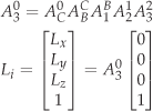
The robot forward kinematics equations allows us to calculate the position of the robot footholds (i.e., L for a given set of 12 joint angles and a $C O G$ vector).

To develop the forward kinematics equations, we use rotation and translation matrices combined in homogeneous transformation matrices. We chose to use the zero reference point (ZRP) [6] representation method, although the Denavit-Hartenberg (DH) [3] method can also be applied. In order to calculate the position of one footpad in the world fixed frame (frame 0), we first transform it to the body fixed frame (frame C). This transition includes the linear translation to the $C_{x}, C_{y}, C_{z}$ coordinates and the rotation matrix describing the three angles of the body tilt in space: $ϕ_{r o l l}, ϕ_{p i t c h}, ϕ_{y a w}$ . We can describe this transformation using the Euler angles [26]:

A_{C}^{0} = [\begin{matrix} c_{p} c_{y} & c_{y} s_{p} s_{r} - c_{r} s_{y} & s_{r} s_{y} + c_{r} c_{y} s_{p} & C_{x} \\ c_{p} s_{y} & c_{r} c_{y} + c_{y} s_{p} s_{r} & c_{r} s_{p} s_{y} - c_{y} s_{r} & C_{y} \\ - s_{p} & c_{p} s_{r} & c_{p} c_{r} & C_{z} \\ 0 & 0 & 0 & 1 \end{matrix}]

(2)

we define $s_{k} ≜ \sin (ϕ_{k}), c_{k} ≜ \cos (ϕ_{k})$

where $k = {r = r o l l, p = p i t c h, y = y a w}$ .

The next transformation will be to the leg's first degree of freedom – the scapula joint. We use the following translation matrix:

A_{B}^{C} = [\begin{matrix} 1 & 0 & 0 & n_{1} \cdot H / 2 \\ 0 & 1 & 0 & n_{2} \cdot W / 2 \\ 0 & 0 & 1 & - l_{0} \\ 0 & 0 & 0 & 1 \end{matrix}]

(3)

where for $\begin{array}{l} L e g_I n d e x = 1 \to n_{1} = n_{2} = 1 \\ L e g_I n d e x = 2 \to n_{1} = 1, n_{2} = - 1 \\ L e g_I n d e x = 3 \to n_{1} = - 1, n_{2} = - 1 \\ L e g_I n d e x = 4 \to n_{1} = - 1, n_{2} = 1 \end{array}$

Now we can describe the rotation of each degree of freedom and the linear translation determined by the lengths of the leg links. The following transformations are shown for a set of angles of a single leg and can be replaced by a set of angles of another leg. A graphical description of the joint angles is shown in Figure 3.

\begin{array}{l} A_{1}^{B} = [\begin{matrix} \cos (θ_{1}) & - \sin (θ_{1}) & 0 & 0 \\ \sin (θ_{1}) & \cos (θ_{1}) & 0 & 0 \\ 0) & 0 & - l_{1} & 0 \\ 0 & 0 & 0 & 1 \end{matrix}] \\ A_{2}^{1} = [\begin{matrix} \cos (θ_{2}) & 0 & - \sin (θ_{2}) & l_{2} \sin (θ_{2}) \\ 0 & 1 & 0 & 0 \\ \sin (θ_{2}) & 0 & \cos (θ_{2}) & - l_{2} \cos (θ_{2}) \\ 0 & 0 & 0 & 1 \end{matrix}] \\ A_{3}^{2} = [\begin{matrix} \cos (θ_{3}) & 0 & - \sin (θ_{3}) & l_{3} \sin (θ_{3}) \\ 0 & 1 & 0 & 0 \\ \sin (θ_{3}) & 0 & \cos (θ_{3}) & - l_{3} \cos (θ_{3}) \\ 0 & 0 & 0 & 1 \end{matrix}] \end{array}

(4)

In order to get the final forward kinematics equations, we multiply the above matrices and multiply the result by ${(0,0,0,1)}^{T}$ . This vector points to the origin of the frame that is attached to the robot footpad (frame 3):

\begin{array}{l} A_{3}^{0} = A_{C}^{0} A_{B}^{C} A_{1}^{B} A_{2}^{1} A_{3}^{2} \\ L_{i} = [\begin{matrix} L_{x} \\ L_{y} \\ L_{z} \\ 1 \end{matrix}] = A_{3}^{0} [\begin{matrix} 0 \\ 0 \\ 0 \\ 1 \end{matrix}] \end{array}

The result allows us to calculate the locations of the robot footpad given the location and orientation angles of the robot body and each joint angle. This calculation is repeated for each leg.

5.2. Inverse Kinematics

The inverse kinematics equations allow us to calculate the actuator angles for a given location of the footpad. In this section, we present the development of the inverse kinematics equations for the presented robot. These equations are very useful in search-based foothold planning algorithms, where a specific point on the ground is considered as a future foothold and where we need to evaluate the joint angles of the moving leg. Unlike the forward kinematics, the inverse kinematics' solution is not injective, and there is more than one solution that satisfies the equations. We can describe each leg as a 3-DOF robotic arm and use the existing inverse kinematics equations from the literature [20]:

\begin{array}{l} k = (L_{B, x})^{2} + {(L_{B, y})}^{2} + {(L_{B, z})}^{2} \\ s = \sqrt{{(L_{B, x})}^{2} + {(L_{B, y})}^{2}} \\ θ_{1} = \arctan (L_{B, y} / L_{B, x}) \\ θ_{2} = \arctan 2 (s, - L_{B, z}) \pm \arccos (\frac{k + l_{2}^{2} - l_{3}^{2}}{2 l_{2} \sqrt{k}}) \\ θ_{3} = \pm (\arccos (\frac{- k + l_{2}^{2} + l_{3}^{2}}{2 l_{2} l_{3}}) - π) \end{array}

(5)

where $L_{B, x}, L_{B, y}$ and $L_{B, z}$ are the components of the vector which points to the footpad from the B frame origin. In order to represent the leg foothold position (which is described in the 0 frame) in the B frame, we first describe the transformation matrix from the 0 frame to the B frame:

A_{B}^{0} = A_{C}^{0} A_{B}^{C} [\begin{matrix} [\begin{matrix} R \end{matrix}] & [\begin{matrix} d \end{matrix}] \\ \begin{matrix} 0 & 0 & 0 \end{matrix} & \begin{matrix} 1 \end{matrix} \end{matrix}]

(6)

where R represents the rotation part and d represents the translation part. We can calculate the inverse transformation matrix as follows:

A_{0}^{B} = [\begin{matrix} [\begin{matrix} R^{T} \end{matrix}] & [\begin{matrix} - R^{T} d \end{matrix}] \\ \begin{matrix} 0 & 0 & 0 \end{matrix} & \begin{matrix} 1 \end{matrix} \end{matrix}]

(7)

Now, we can calculate the desired vector which points to the leg footpad from the origin of frame B (the scapula joint):

[\begin{matrix} L_{B, x} \\ L_{B, y} \\ L_{B, z} \\ 1 \end{matrix}] = A_{0}^{B} \cdot L_{i}

(8)

By using the inverse kinematics, a foothold-planning algorithm can convert the required foothold location into actuator angles in order to command the robot to move. In addition, the inverse kinematics' calculation can be used to rule out foothold locations that are considered to be kinematically impossible (i.e., if the calculated angles result in a complex number or an angle greater than the robot's physical design limitations).

5.3. The Robot Workspace

The robot motion is divided into two phases: body movement and leg movement. During the body movement phase, all four footpads are stationary and the body workspace comprises the six parameters of the COG vector. During the leg movement phase, the robot body is fixed and the leg's workspace includes all possible locations of a moving leg's footpad, which are the $L_{i}$ parameters. The robot body workspace is the set of all the possible locations and orientations of the robot body given the legs' footholds. In general, this is a six-dimensional space. For a given body orientation angle, this is a three-dimensional space which spans all the possible $C_{x}, C_{y}$ and $C_{z}$ coordinates. This workspace can be calculated analytically using the robot inverse kinematics equations that describe the location of the centre of gravity of the robot, but the direct calculation of the inverse kinematics equations is computationally intensive. Figure 6 shows the workspace of the robot for a horizontal body and a height of 20 cm.

Figure 6.

The robot body workspace

The robot leg workspace is the set of all the possible locations of the robot footpad for a given position and orientation of the robot's body. This workspace can be calculated using the robot kinematics equations. An alternative, more intuitive, method which requires less computing resources is based on investigating the geometry of a leg's joints. The two bottom degrees of freedom of a leg, $θ_{2}$ and $θ_{3}$ , are in the same plane and spanning an area in the shape of a ring with its centre in the rotation axis of $θ_{2}$ . These ring radii are:

\begin{array}{l} R_{\max} = l_{2} + l_{3} \\ R_{\min} = \sqrt{l_{2}^{2} + l_{3}^{2} - 2 l_{2} l_{3} \cos (π - θ_{3_L i m i t})} \end{array}

(9)

where $θ_{3_L i m i t}$ is the physical limitation of the $θ_{3}$ actuator limit angle. The leg upper degree of freedom, $θ_{1}$ , spins this ring around the $l_{1}$ link axis and creates a spherical shell with a thickness of $R_{m a x} - R_{m i n}$ . The workspace is also limited by $θ_{2_L i m i t}$ . We can visualize this limitation as a cone with its head at the ring centre, an angle of $θ_{2_L i m i t}$ and an infinite height in the direction of the $l_{1}$ link axis. The intersection volume between the sphere and the cone is the leg workspace, as can be seen in figures 7(a) and 7(b):

Figure 7.

Leg Workspace in 3D (a), and from a side view (b)

Figure 8.

Illustration of the motion capture system

This workspace can be used in order to determine what areas in the ground should be take into account when searching for the footholds' locations. From Figure 7 (b), we can see a maximum stride length of 20 cm while maintaining the body in the presented posture.

6. Experimental Results

Experiments were conducted to demonstrate and verify the design and kinematics computations. We chose the OptiTrack motion capture system by NaturalPoint in order to quantify the results of the experiment. The system consists of 12 cameras radiating infrared light and measuring the reflection from passive markers located on the robot. Information from all the cameras is processed on a computer, which calculates the exact position of each marker. The more cameras that detect the same marker, the greater the accuracy in calculating the position. We present the results of three experiments. The first experiment verifies the motion of the robot leg. The second experiment shows the robot body's manoeuvring capabilities while keeping all four legs' footholds stationary. The final experiment demonstrates an entire walking sequence.

Figure 9 shows how the markers are attached to the robot.

Figure 9.

The placement of the markers on the robot

6.1. Leg motion experiment

This experiment examines the performance of the robot legs. The robot moved according to a sequence of commands. The commands changed the three actuators of one leg ( $θ_{1}, θ_{2}$ and $θ_{3}$ ) while the robot was standing stably on the other three legs. The robot body configuration for this experiment was:

\begin{array}{l} C O G = (C_{x}, C_{y}, C_{z}, ϕ_{r o l l}, ϕ_{p i t c h}, ϕ_{y a w}) = \\ (0,0,22 [c m {],0}^{\circ} {,0}^{\circ} {,0}^{\circ}) . \end{array}

The command sequence and the respective forward kinematics is shown in Table 3.

Table 3.

Leg motion experiment command sequence

Command	$θ_{1} [^{\circ}]$	$θ_{2} [^{\circ}]$	$θ_{3} [^{\circ}]$	$L_{1_{x}} [c m]$	$L_{1_{y}} [c m]$	$L_{1_{z}} [c m]$
0	0	45	65	28.54	12.25	14.16
1	0	90	0	32.25	12.25	18
2	45	45	−90	11.25	12.25	3.15
3	90	90	45	11.25	30.17	25.42
4	0	0	75	21.39	12.25	4.78

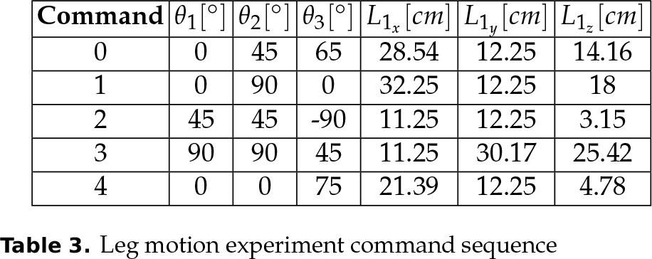
where command 0 is the initial state. All commands were sent with an interpolation time of five seconds. The interpolation time comprises the time taken for all the motors to complete the motion as described in Section 3. The results of this experiment are shown in Figure 10. In the figure, the actual path of the footpad is presented while moving between the desired via point of Table 3.

Figure 10.

Leg motion experiment results according to the joints angles described in Table 3. The desired footpad locations are marked in red dots and the actual footpad path is the blue curve.

The position error of the footpad with respect to the desired position after each command is shown in Table 4:

Table 4.

Leg motion experiment distance errors

Command	Error $[c m]$
0	0.22
1	0.24
2	0.37
3	0.84
4	0.35

The mean error is 0.4061 cm, which is reasonable considering a marker size of 1 cm.

6.2. Body manoeuvring experiment

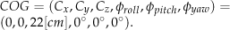
This experiment examined the robot body's manoeuvrability. We use the robot inverse kinematics in order to send commands which control the robot configuration but which do not control the actuator angles directly. That is, the desired motion is the body position and orientation movement. The experiment validated the inverse kinematics model and the robot's ability to control all the actuators simultaneously. We divided this experiment into two parts, one for position movement and a second for orientation movement. In the first part of the experiment, part (a), we changed the $C_{x}, C_{y}$ and $C_{z}$ sequentially. First $C_{x}$ moved by 2 cm in each direction (forwards and backwards), then $C_{y}$ moved by 2 cm in each direction (left and right), and then $C_{z}$ moved by 2 cm in each direction (up and down). The interpolation times for each command were set automatically while making sure that the maximum actuator speed did not exceed 0.01 degrees per second. This speed limit constraint determines the interpolation time by limiting the speed of the motor with the longest path. The results are presented in Figures 11(a) and 11(b).

Figure 11.

Body manoeuvring experiment, part (a) results: body position vs time in (a) and body orientation angles vs time in (b)

Figure 12.

Body manoeuvring experiment, part (b) results

As shown in Figure 11(a), the robot completes its task with a maximum position error of 0.6 cm between the desired and actual body positions. We substitute the initial height of the robot from the original z measurements in order to emphasize the movement with respect to the initial position. The reason for the deviations in the x curve is that the commands sent to the robot included the target points for each motor and not the complete motion profile. A possible solution to this problem is to divide the complete path into a set of short movements between points along a desired path. This solution would ensure that the robot's actual path remains close enough to the desired path. Figure 11(b) shows that the robot maintained its body level horizontally as well as maintaining the yaw angle. The mean absolute errors for the roll pitch and yaw angle are ${0.29}^{\circ}$ , ${0.24}^{\circ}$ and ${0.2}^{\circ}$ respectively. In the second part of this experiment, part (b), we will change the orientation angles of the body, $ϕ_{r o l l}, ϕ_{p i t c h}$ and $ϕ_{y a w}$ , each by $5^{\circ}$ in both directions. The results are presented in Figure 12.

As shown, the robot performs the manoeuvre adequately. The mean absolute errors during the entire manoeuvre for the roll pitch and yaw angles are ${0.25}^{\circ}$ , ${0.33}^{\circ}$ and ${0.19}^{\circ}$ degrees respectively. From Figures 11 (a) and 12, one can see that the execution time of the motion in different directions is not the same. For example, it can be seen that the manoeuvres in the x direction and the pitch angle are faster than the motion in other directions. The reason for this lies in the configuration of the robot legs. While in the starting posture, the axes of the two lower motors are parallel to the y axis, and there is no need to move the upper leg motors in order to perform movement in the x and pitch manoeuvres. Moving in other directions requires more motors to move a longer distance.

6.3. Walking experiment

The last experiment demonstrated the robot's performance during walking. We used the foothold planning algorithm from [5] to generate a set of double steps in which the robot advanced in a straight line over a flat ground surface. A double step consists of one movement of the robot body and then a sequence movement of the two legs. The foothold planning algorithm uses a search-based method to scan all possible steps and a graph search algorithm to plan and select the future steps. This is a free-gait generator rather than a cyclic gait generator. The provision of further details of the gait generator is beyond the scope of this paper and can be found in [5]. The results of the experiment are presented in Figure 13.

Figure 13.

Walking experiment results: required an actual path in (a); initial and final positions in (b); and position vs time in (c)

Figure 13(a) presents the required centre of gravity path as received from the foothold planning algorithm and the actual path as recorded with the motion capture system. The robot followed the desired path up to a mean absolute error of 0.39 cm. We observed that the actual path does not form a straight line between the $C O G$ target points along the required path. This is the same phenomenon as described in the body manoeuvring experiment. To reduce the effect of this phenomenon, we divided each path between two $C O G$ target points into four segments. Still, we can see small deviations from the required path. The entire motion planning of the robot was pre-calculated (offline); hence, the progress of the robot is in a open loop and so we do not feed back the real configuration in real-time. In Figure 13(c), we present the time history of the x and y coordinates. Since every movement is segmented into four parts, it result in a non-smooth path, as shown in the Figure. The robot's average forward speed during the motion is 0.3 cm/sec. Note that in this experiment we used a slow speed motion and a non-optimal gait. We believe it is possible to increase the speed dramatically. More experiments are needed in order to determine the maximum available performance characteristics. To analyse the stability of the robot, we present the support polygons [19] for all stages of the walking motion. The support polygon is the horizontal projection of the polygon composed from the supporting legs' footpads – in our case (a quadruped walking under equilibrium constraints), the polygon is a triangle during leg movement. As seen in Figure 14, in each double step sequence, two steps are performed using different legs while the body is stationary. During every double step, the centre of gravity (marked with a green circle) is inside the support polygons (dashed magenta lines). While planning the motion, we used a stability margin requiring a distance of at least 3 cm between the horizontal projection of the centre of gravity and the support polygon edges. We used this distance considering the 2.2 cm uncertainty in the centre of mass position caused by the mass of the robot legs.

Figure 14.

Walking experiment results. Presenting the support polygons for all four steps in chronological order from (a) to (d).

During the experiment, the power consumption of the robot was measured. The robot consumed 14[W] while standing still and an average of 20[W] while walking, with a peak of 32[W]. The battery is rated as 31.1[Wh]; therefore it can power the robot for more than one hour of continuous walking.

7. Conclusions

We introduced a novel design of a quadruped robot for research purposes. We presented both hardware and software designs as well as a robot kinematics model. Validation experiments were performed and the results show the robot's movement according to a predefined path, with a mean absolute motion error of 0.6 cm linearly and a ${0.33}^{\circ}$ angular error. The main advantages of the robot design are simplicity, modularity, a simple interface and low cost. We believe that such a robotic platform can significantly accelerate advances in research on four-legged walking robots. Future work will include the design of a robot with a 3D scanning sensor and a more powerful processing unit, and which is capable of processing the information from the scanning sensor and implementing more complex control of the robot actuators. Our goal hardware for this future design is the ASUS Xtion PRO LIVE as the 3D scanning sensor and the BeagleBoard as the computation unit. The weight-carrying capacity of the robot allows for the addition of additional sensors in the future, such as inertial measurement units, laser scanners and footpad force sensors. A future goal will be to enable the robot to autonomously navigate through rough terrain, as shown in Figure 15. Future work will also include dynamic locomotion to allow the robot to run, jump and avoid dynamic obstacles.

Figure 15.

The robot

Footnotes

1

SolidWorks is a registered trademark of Dassault Systèmes

2

MATLAB is a registered trademark of The MathWorks, Inc.

8. Acknowledgements

This work was partially supported by the Israeli Ministry of Defence grant no. 8522033, The Pearlstone Centre of Aeronautical Engineering Studies, and the Paul Ivanier Centre for Robotics Research and Production Management.

References

Lucas

Huitieme recreation – la machine a marcher. Recreat. Math 4, pages 198–204, 1894.

Mcghee

R. B.

and Frank

A. A.

On the stability properties of quadruped creeping gaits. Mathematical Biosciences, 3(1-2):331–351, August 1968.

Iida

Gomez

, and Pfeifer

Exploiting body dynamics for controlling a running quadruped robot. In Advanced Robotics, 2005. ICAR '05. Proceedings., 12th International Conference on, pages 229–235, 2005.

Kikuchi

Ota

, and Hirose

Basic performance experiments for jumping quadruped. In Intelligent Robots and Systems, 2003. (IROS 2003). Proceedings. 2003 IEEE/RSJ International Conference on, volume 4, pages 3378 – 3383 vol.3, oct. 2003.

Shapiro

Rimon

, and Shoval

. A foothold selection algorithm for spider robot locomotion in planar tunnel environments. The International Journal of Robotics Research, 24(10):823–844, 2005.

Sintov

Avramovich

, and Shapiro

Design and motion planning of an autonomous climbing robot with claws. Robotics and Autonomous Systems, 59(11):1008–1019, 2011.

Kolter

J. Z.

and Ng

A. Y.

The stanford littledog: A learning and rapid replanning approach to quadruped locomotion. Int. J. Rob. Res., 30(2):150–174, 2011.

Bretl

Lall

Latombe

, and Rock

Multi-step motion planning for free-climbing robots. In in WAFR, pages 1–16, 2004.

Igarashi

Machida

Harashima

, and Kakikura

Free gait for quadruped robots with posture control. In 9th IEEE International Workshop on Advanced Motion Control, pages 433–438, 2006.

10.

Igarashi

and Kakikura

Path and posture planning for walking robots by artificial potential field method. In IEEE International Conference on Robotics and Automation, 2004. Proceedings. ICRA '04. 2004, volume 3, pages 2165–2170, may 2004.

11.

Kolter

J. Z.

Rodgers

M. P.

, and Ng

A. Y.

A control architecture for quadruped locomotion over rough terrain. In IEEE International Conference on Robotics and Automation, 2008. ICRA 2008., pages 811–818, may 2008.

12.

Estremera

and de Santos

P. G.

Generating continuous free crab gaits for quadruped robots on irregular terrain. IEEE Transactions on Robotics, 21(6):1067–1076, 2005.

13.

Rimon

Shoval

, and Shapiro

Design of a quadruped robot for motion with quasistatic force constraints. Autonomous Robots, 10:279–296, 2001.

14.

Kalakrishnan

Buchli

Pastor

Mistry

, and Schaal

Learning, planning, and control for quadruped locomotion over challenging terrain. The International Journal of Robotics Research, 30(2):236–258, 2011.

15.

Buchli

and Ijspeert

Self-organized adaptive legged locomotion in a compliant quadruped robot. Autonomous Robots, 25(4):331–347, 2008.

16.

http://www.bostondynamics.com/robot_littledog.html, Accessed on 01 April 2013.

17.

Hutter

Gehring

Bloesch

Hoepflinger

M. A.

Remy

C. D.

, and Siegwart

StarlETH: A compliant quadrupedal robot for fast, efficient, and versatile locomotion. In 15th International Conference on Climbing and Walking Robot – CLAWAR 2012, 2012.

18.

Remy

Baur

Latta

Lauber

Hutter

Hoepflinger

Pradalier

, and Siegwart

Walking and crawling with ALoF: a robot for autonomous locomotion on four legs. Industrial Robot: An International Journal, 38(3):264–268, 2011.

19.

Kato

and Hirose

Development of the quadruped walking robot, titan-ix – mechanical design concept and application for the humanitarian de-mining robot. Advanced Robotics, 15(2):191–204, 2001.

20.

Kang

Kim

Son

, and Choi

Design of quadruped walking and climbing robot. In Intelligent Robots and Systems, 2003. (IROS 2003). Proceedings. 2003 IEEE/RSJ International Conference on, volume 1, pages 619–624, 2003.

21.

Rimon

Shoval

, and Shapiro

Design of a quadruped robot for motion with quasistatic force constraints. Autonomous Robots, 10(3):279–296, 2001.

22.

Loc

V-G

Koo

I. M.

Tran

D. T.

Park

Moon

, and Choi

H. R.

Improving traversability of quadruped walking robots using body movement in 3d rough terrains. Robotics and Autonomous Systems, 59(12):1036–1048, August 2011.

23.

Koo

I. M.

Trong

T. D.

Lee

Y. H.

Moon

, and Choi

H. R.

Control of quadruped walking robot aidin-iii based on biomimetic inspired approach. In The 6th Asian Conference on Multibody Dynamics(ACMD), August 2012.

24.

Robotis, Dynamixel RX-64 Robot Actuator, http://www.robotis.com/xe/dynamixel_en, Accessed on 01 April 2013.

25.

Robotis, Dynamixel Frames, http://www.robotis.com/xe/dynamixel_en, Accessed on 01 April 2013.

26.

http://www.vanadiumlabs.com/arbotix.html Vanadium Labs, ArbotiX Robocontroller, http://www.vanadiumlabs.com/arbotix.html, Accessed on 01 April 2013.

27.

Vanadium Labs, ArbotiX RX-Bridge, http://www.vanadiumlabs.com/rx.html, Accessed on 01 April 2013.

28.

Digi International Inc, XBee 2.4 GHz RF Module, http://www.digi.com/products/wireless-wired-embedded-solutions/zigbee-rf-modules/point-multipoint-rfmodules/xbee-series1-module, Accessed on 01 April 2013.

29.

Vanadium Labs, BioloidController library, http://code.google.com/p/arbotix/wiki/BioloidController, Accessed on 01 April 2013.

30.

Garage

“Robot Operating System”, http://www.ros.org. Accessed on 01 April 2013.

31.

Gupta

K. C.

Kinematic analysis of manipulators using the zero reference position description. The International Journal of Robotics Research, 5(2):5–13, 1986.

32.

Denavit

and Hartenberg

R. S.

A kinematic notation for lower-pair mechanisms based on matrices. Trans. of the ASME. Journal of Applied Mechanics, 22:215–221, 1955.

33.

Spong

M. W.

Robot Modeling and Control. WILEY Publication, 2005.

34.

Murray

R. M.

, and Sastry

S. S.

A Mathematical Introduction to Robotic Manipulation. 1994.

35.

Geva

and Shapiro

A combined potential function and graph search approach for free gait generation of quadruped robots. In Robotics and Automation (ICRA), 2012 IEEE International Conference on, 2012.

A Novel Design of a Quadruped Robot for Research Purposes

Abstract

Keywords

1. Introduction

2. Quadruped Robot Design

3. Control and Communication

4. Robot Cost

5. Kinematics Analysis

5.1. Forward Kinematics

5.2. Inverse Kinematics

5.3. The Robot Workspace

6. Experimental Results

6.1. Leg motion experiment

6.2. Body manoeuvring experiment

6.3. Walking experiment

7. Conclusions

Footnotes

1

2

8. Acknowledgements

References