Sage Journals: Discover world-class research

Abstract

Mobile sensor networks are an important part of modern robotics systems and are widely used in robotics applications. Therefore, sensor deployment is a key issue in current robotics systems research. Since it is one of the most popular deployment methods, in recent years the virtual force algorithm has been studied in detail by many scientists. In this paper, we focus on the virtual force algorithm and present a corresponding parameter investigation for mobile sensor deployment. We introduce an optimized virtual force algorithm based on the exchange force, in which a new shielding rule grounded in Delaunay triangulation is adopted. The algorithm employs a new performance metric called ‘pair-correlation diversion', designed to evaluate the uniformity and topology of the sensor distribution. We also discuss the implementation of the algorithm's computation and analyse the influence of experimental parameters on the algorithm. Our results indicate that the area ratio, φ_s, and the exchange force constant, G, influence the final performance of the sensor deployment in terms of the coverage rate, the convergence time and topology uniformity. Using simulations, we were able to verify the effectiveness of our algorithm and we obtained an optimal region for the (φ_s, G)-parameter space which, in the future, could be utilized as an aid for experiments in robotic sensor deployment.

Keywords

Wireless Sensor Networks Virtual Force Algorithm Delaunay Triangulation Pair-correlation Diversion

1. Introduction

With the development of information technology, nowadays robots play a key role in industrial manufacturing, intelligence services and military assistance. Many scientists are currently conducting research and development in robotics applications. Due to the fact that informational sensors have become more efficient and inexpensive over time, mobile wireless sensor networks (WSNs) have been assigned an important role in autonomous robots with sensing and communication abilities. Mobile sensors collect a variety of data based on a distributed network that have the advantages of low power consumption, low cost, high reliability and self-organization. Such networks are widely used in robotics technology and in applications such as range sensing, target tracking, robot control, robot vision and environment monitoring, etc. [1].

Sensor deployment algorithms can be categorized as either deterministic or movement-assisted [2]. In special environments (e.g., remote or unmanned cases), sensor nodes are randomly distributed and only movement-assisted deployment can be applied. Since a good deployment method can offer robotics applications higher flexibility, practicability and adaptivity, deploying mobile sensors effectively is a key issue in current robotics WSN research. In general, in deployment algorithms for mobile sensor networks, each sensor knows its position, can communicate with other nodes, and can move to a better position according to collected or computed information in order to improve the coverage rate. Good intelligent deployment algorithms mainly include the following aspects: (1) processes to save sensor energy to extend the lifetime of network systems; (2) processes to obtain a uniform network topology in order to enlarge the coverage area; and (3) processes for accelerating the entire deployment procedure. Many approaches have been proposed for robotics sensor network deployment that have their own advantages, including: (1) computational geometry and grid-based methods [3–5]; (2) virtual force- or potential-based strategies [6–15]; (3) swarm intelligence and bionics algorithms [16–23]; and/or (4) a combination of the above approaches [24–26].

Among the above methods, virtual force-based strategies have been deemed effective, are popular and have become a hot topic in WSN research for robotics systems over the last decade. Recently, Zou and Chakrabarty presented a virtual force algorithm (VFA) using attractive and repulsive forces in order to determine the virtual motion paths and movement rates of sensor nodes. They also proposed a probabilistic target localization algorithm that can maximize the sensor field coverage [7]. To increase the robustness of the robot sensor network, Kribi et al. reported a serialized VFA with good coverage, connectivity and fault-tolerance [9]. Garetto et al. investigated a distributed sensor relocation algorithm based on virtual force for environmental control that can provide regular tessellation for a given geographical area. The algorithm provides an effective distributed method as compared with an optimal centralized solution [10]. Yu et al. proposed a new sensor deployment algorithm based on Van der Waals [12] and the virtual spring force [14]. The spring force-based algorithm resulted in proper damping for the deployment of sensor nodes in mobile WSNs [14]. Yuαŕs methods are capable of supplying a better coverage rate, more uniformity for the network configuration, and a moderate convergence time. Moreover, a novel VFA based on physical laws for a dusty plasma system was presented by Wen et al. The method is capable of forming an hexagonal topology in wireless sensor networks. These authors also introduced a performance metric based on the pair-correlation function in a crystal structure in order to evaluate the similarity between sensor network topologies resulting from the VFA and a perfect hexagonal structure [15]. The algorithm provides maximum field coverage with a minimum system cost.

Here, based on the work of Garetto, we report modifications and improvements for the basic VFA [10]. We first describe changes to the shielding rule using Delaunay triangulation in order to replace the original shielding rule that determines the adjacent nodes of a given node. Second, to evaluate the uniformity of the node distribution, a new performance evaluation metric (improved from paper [14, 15]) is introduced. Our simulation results indicate that the approach exhibits good performance in terms of the convergence time and uniformity for the network configuration. We also provide a detailed discussion of the factors influencing our algorithm and obtain an optimal region for the (φ_s,G)-parameter space.

The paper is organized as follows. In Section 2, we introduce the basic concept of the VFA and present our optimized node deployment solution, where we propose a new shielding rule for our algorithm and improve the metrics in order to evaluate it. In Section 3, we simply describe the implementation routine for our algorithm. Simulation results and discussions are provided in Section 4. We also verify the effectiveness of our algorithm and provide a detailed analysis of the corresponding parameter effects. Concluding remarks are provided in Section 5.

2. The Optimized Node Deployment Algorithm

2.1 Review of the VFA

Since each sensor node is regarded as a particle in the robotic sensor network, the virtual force algorithm is influenced by interactions among the particles of the physical system. In general, two assumptions are made in the physical system [7], as follows: (1) Each sensor node has a sensing radius, R_s, and a communication radius, R_c, (R_s ≪ R_c). Within the sensing range, the sensor can detect local environmental conditions and can communicate with other nodes that fall into its communication range. (2) The position of all the nodes can be determined using various methods (e.g., GPS). All of the nodes can effectively move according to the calculation results of the algorithm. Thus, all of the nodes should eventually reach equilibrium through interactions of the virtual forces and form a stable lattice structure that corresponds to a sensor network topology.

Here, we adopt a second-order differential equation for node motion in the VFA [10, 14], whose nodes are subjected to variable motion because the second-order differential equation is normally easier to determine in dynamic equilibrium in a physical system. The equation of a given node i is as follows,

m \frac{d^{2} r_{i} (t)}{d t^{2}} = F_{i} (t) = F_{i}^{e} (t) + F_{i}^{f} (t),

(1)

where m is the virtual mass of a sensor node, F _i^e(t) is the total exchange force emerging from the other nodes, and F _i^f (t) is the friction force that reduces the node velocity to reach an equilibrium state. We describe these two forces in the following discussion [10].

1. Exchange forces F _i^e(t)

When the distance d_ik(t) between two given nodes i and k at time t is less than the communication radius R_c, there is an exchange force between the two nodes. If A(i,t) is the set of nodes acting with exchange forces on node i at time t, then k ∊ A(i,t). We define the formula for total exchange forces on node i at time t as

F_{i}^{e} (t) = \sum_{k \in A (i, t)} G \frac{(d_{i k} (t) - D_{m})}{d_{i k} (t) (R_{c} - d_{i k} (t))} {\hat{r}}_{i k} (t),

(2)

where ${\hat{r}}_{i k} (t)$ is the normalized vector of r _ik(t), D_m is the equilibrium distance and G is a constant that significantly affects the node speed. When G is too small, the initial node speed is small and the system takes more time to achieve convergence. When G is too large, the node speed is so large that all the nodes fluctuate around the equilibrium state. The result is a bad convergence rate and weak deployment performance.

2. Friction forces F _i^f (t)

The friction forces acting on a node i at time t can be written as

F_{i}^{f} (t) = (\begin{matrix} - \min (k_{0} {\hat{F}}_{i}^{e} (t), F_{i}^{e} (t)), if v_{i} (t) = 0 \\ - k_{υ} v_{i} (t), if v_{i} (t) \neq 0 \end{matrix},

(3)

where ${\hat{F}}_{i}^{e} (t)$ is the normalized vector of F _i^e(t), v_i(t) is the velocity of node i, k₀ is the static friction factor and k_v is the viscous friction factor. When v_i(t) = 0, the static Coulomb friction $- k_{0} {\hat{F}}_{i}^{e} (t)$ suppresses the movement of node i. When v_i(t) ≠ 0, the viscous friction −k_vv_i(t) decreases the velocity of node i.

At the beginning of our algorithm, when the initial nodes are randomly deployed, all of the nodes are stationary. We then compare F _i^e(t) and $k_{0} {\hat{F}}_{i}^{e} (t)$ for all of the nodes. If $| F_{i}^{e} (t) | > | k_{0} {\hat{F}}_{i}^{e} (t) |$ , the node begins to move along the direction of the total virtual force. During the movement process, viscous friction continues to decrease the velocity of the nodes. When the velocity of a node is reduced to zero, we repeat the previous comparison and the movement procedures until $| F_{i}^{e} (t) | \leq | k_{0} {\hat{F}}_{i}^{e} (t) |$ . Finally, when all of the nodes achieve a force balance - indicating zero resultant force - we consider the entire sensor network to have been successfully deployed; $k_{0} {\hat{F}}_{i}^{e} (t)$ also acts as a threshold for system balance. In general, to achieve the best computation result, the value of $k_{0} {\hat{F}}_{i}^{e} (t)$ should be a small value.

2.2 Optimization of the Shielding Rule

In general, the issue of how to define adjacent nodes of a given node will determine the computational complexity of the total virtual force in a VFA simulation. Thus, a good shielding rule used to restrict adjacent nodes plays a key role in improving and simplifying the entire algorithm.

In a perfect hexagonal network topology, each node should be surrounded by six adjacentnodes. When the equilibrium distance D_m = √3R_s, the sensor network ideally forms a triangular tessellation and can yield the optimal hexagonal coverage [10, 15]. Garetto et al. introduced a shielding rule as follows: If k and k’ are two nodes within the communication range of node i, node k’ shields k only if k’ is closer to i and the angle formed by the vectors r _ik, and r _ik is smaller than 60° [10]. Under this shielding rule, six nodes, at most, can simultaneously act on node i. In general, the number of computed adjacent nodes is not more than six.

Therefore, we present a new method for optimizing the shielding rule. We generate Delaunay triangulation in order to accurately ascribe all of the neighbours of each node. A Delaunay triangulation for a set of points P in a plane is a triangulation DT(P) such that no point in P is inside the circumcircle of any triangle in DT(P). The method maximizes the minimum angle for all of the angles of the triangles in the triangulation, which tends to avoid skinny triangles [27]. Yu et al. introduced this method into WSN applications and presented its effectiveness in adjacent node analysis [11].

We let A_nei(i,t) be the set of first-round adjacent nodes surrounding node i generated by Delaunay triangulation at time t. We then computed the total virtual force from these accurate nodes in the set A(i,t)∩A_nei(i,t). Formula (2) can then be rewritten as:

F_{i}^{e} (t) = \sum_{k \in A (i, t) \cap A_{n e i} (i, t)} G \frac{(d_{i k} (t) - D_{m})}{d_{i k} (t) (R_{c} - d_{i k} (t))} {\hat{r}}_{i k} (t) .

(4)

Since Delaunay triangulation can accurately determine the adjacent relationship of all the nodes, it is a useful tool for investigating the total force acting from second- or third-round adjacent nodes and - later on - enlarging the shielding range.

2.3 Performance Evaluation of the VFA

To objectively evaluate the performance of various VFAs, assessing performance from different perspectives is essential. Based on research on crystallization in a dusty plasma [28, 29], Wen et al. introduced a novel performance metric, known as the pair-correlation diversion (PCD), in order to evaluate the proximity between any network coverage topology and a perfect hexagonal topology [15]. The method is based on the pair-correlation function, g(r) = (N(r,Δ)S)/(2πrΔN), in a crystalline structure and represents the probability of finding two nodes separated by a distance r. In the equation, S is the area occupied by a 2D system, N is the number of nodes contained in S, and N(r,Δ) indicates the number of nodes located between r − Δ/2 and r + Δ/2 (see references [14, 15, 29] for details). The PCD works well when the node density of the sensor network is close to the node density of a perfect hexagonal configuration, but not so well when the node density is too large or too small.

Here, we make improvements to the PCD in order to evaluate the uniformity of the network configuration. Based on the definition of g(r), we further improve the performance metric formula as follows,

δ (Ω, Ω_{H}) = \frac{\int_{0}^{r_{T}} {‖ g_{Ω} (r) - g_{Ω_{H} (r)} ‖}^{2} d r}{\int_{0}^{r_{T}} {‖ g_{Ω} (r) + g_{Ω_{H} (r)} ‖}^{2} d r},

(5)

where Ω is the network topology to be analysed, Ω_H is the perfect hexagonal topology, and r_T is the bound of the radial distance. For a sensor network, when the value of δ(Ω,Ω_H) is small, the network coverage topology will approximate a perfect hexagonal structure. A perfect network configuration has a δ(Ω,Ω_H) value close to zero. Moreover, δ(Ω,Ω_H) can be applied in order to characterize the convergence rate of a VFA. Beginning with an initial node distribution, δ(Ω,Ω_H) decreases while the deployment progresses over time. When the network reaches the equilibrium state, the value becomes stable. We can then use the slope of the PCD function over the convergence time in order to specify the convergence rate.

3. The Optimized VFA Implementation Routine

In this section, we describe our implementation routine for the optimized VFA. At the beginning of the simulation, we pre-configure values for the initial parameters required for the configuration. Considering that N nodes are deployed in a circular area, S, the main process of the algorithm is as follows:

Set the centre of S at (0,0). Initially, N sensor nodes are randomly distributed within a circular area, S_init, and the location of node i is r _i = (x_i,y_i) where i = 1, 2, ⋅⋅⋅, N. All of the nodes have v₀ = 0 when t₀ = 0.

Use the Bowyer-Watson algorithm [30] in order to generate a Delaunay triangulation and obtain a relational structure among the nodes; then, choose the first-round of adjacent nodes for each node i.

Cyclically execute the following three steps for all of the sensor nodes i (i = 1,2, ⋅⋅⋅, N), as follows:

Calculate the distance between node i and the adjacent node in A_nei(i,t), such as d_ik. If d_ik > R_c, abandon the value. Rest nodes are located in A(i,t) ∩ A_nei(i,t).

Combine formulae (4) and (3) in order to calculate the virtual force and the acceleration, expressed as a _i of node i.

Use leapfrog integration in order to calculate the new velocity and the displacement of node i after time step dt; then, update the original velocity and the displacement. If the velocity of node i exceeds V_max’ set it to V_max.

Repeat Steps 2 and 3 in order to calculate the acceleration, velocity and displacement for all of the nodes after each time step dt until the system reaches the equilibrium state.

4. Simulation Results and Discussion

In this section, to verify the effectiveness of the algorithm and to give details regarding the influence of experimental parameters on the optimized VFA, we provide our simulation results.

4.1 Effectiveness Verification

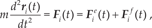
Using the parameters employed by Garetto et al. [10], we modified R_s = 1, R_c = 3 and D_m = √3. Theoretically, the optimal coverage range is approximate to S_perf = N D_m²√3/2 (about N hexagonal area, ignoring the approximate border). We used G = 0.1, k₀ = 1.0e − 5, k_v = 0.1, V_max = 0.01 and dt = 1.0 as the initial parameters. For N = 500, all of the sensor nodes were randomly distributed around the centre of the deployment area. We choose an initial distribution area of S_init = 0.7S_perf = 525√3.

In Figure 1, we provide the initial distribution and the final distribution when the network reached an equilibrium state. The black point indicates a single sensor node and the blue circle indicates its sensing range. Obviously, the final network achieved a uniform configuration and a good coverage.

Figure 1.

The initial node distribution locations (left) and the final distribution locations (right)

In Figure 2, we plot the Delaunay triangulation and the dual graph Voronoi diagram for the final network configuration. The green lines clearly indicate the triangular tessellation generated by Delaunay triangulation, and the blue-line structure generated by the Voronoi diagram provides a very good hexagonal coverage topology.

Figure 2.

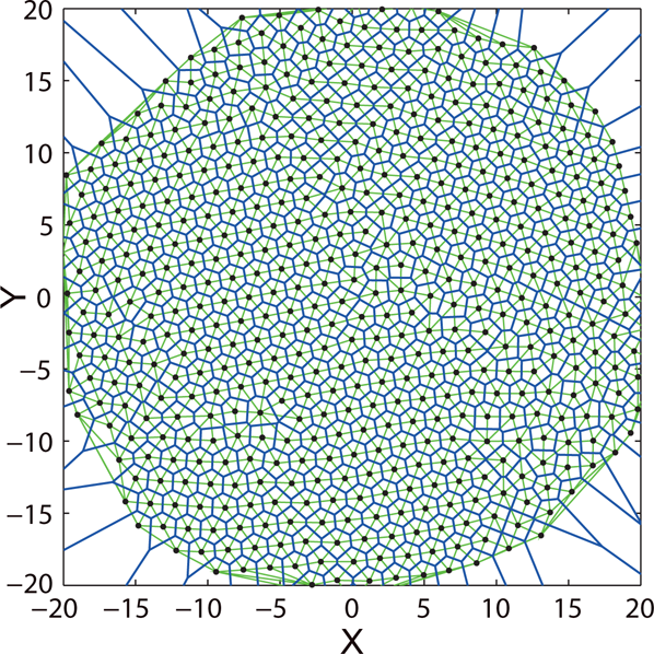
The final network coverage topology represented by the Delaunay triangulation method

In Figure 3, we present the PCD curve along the calculation time step. We determined that VFA-DT reached an equilibrium state after 1,150 time steps and that the corresponding δ(Ω,Ω_H) = 0.158. However, VFA-LJ required 1,900 time steps and the corresponding δ(Ω,Ω_H) = 0.206. The results indicate that VFA-DT converged faster than VFA-LJ and that the final distribution of VFA-DT was more approximate to a perfect hexagonal topology, which also means that our algorithm can obtain a better convergence time and uniformity compared with the general VFA of Garetto et al. [10].

Figure 3.

A performance evaluation curve for δ(Ω,Ω_H) as a function of the time step, as determined from our optimized algorithm (VFA-DT) and the algorithm (VFA-LJ) of Garetto et al.[10]

4.2 Influence of the Initial Node Density

Previously, we arbitrarily chose S_init = 0.7S_perf to verify our algorithm, although we know that S_init also indicates the node deployment density, according to ρ = N / S, for a fixed node number, N. In an actual experiment, the node deployment area is easy to identify, so below we adjust the initial distribution area, S_init, in order to discuss the influence of different node densities on sensor deployment. In general, ρ_init = N / S_init reflects the degree of sparseness for the sensor nodes. If ρ_init is too large, the nodes should move a longer distance in order to be steady, and the convergence time should decrease with high energy consumption. If ρ_init is too small, blank monitoring areas may appear after the sensors are deployed. The area is only a local optimum but not a global optimum.

By setting the ratio φ_s = S_init / S_perf and keeping the other parameters the same, as in Section 4.1, in Figure 4 we present typical profiles for the PCD value δ(Ω,Ω_H) as a function of the time step for cases φ_s = 0.1,0.2, ⋅⋅⋅, 1.2.

Figure 4.

Typical profiles for PCD δ(Ω,Ω_H) as a function of the time step for specified values of φ_s

In Figure 5, based on the results provided in Figure 4, we plot the convergence time and the PCD value δ(Ω,Ω_H) as a function of φ_s using a cubic spline interpolation when the system first reaches the equilibrium state.

Figure 5.

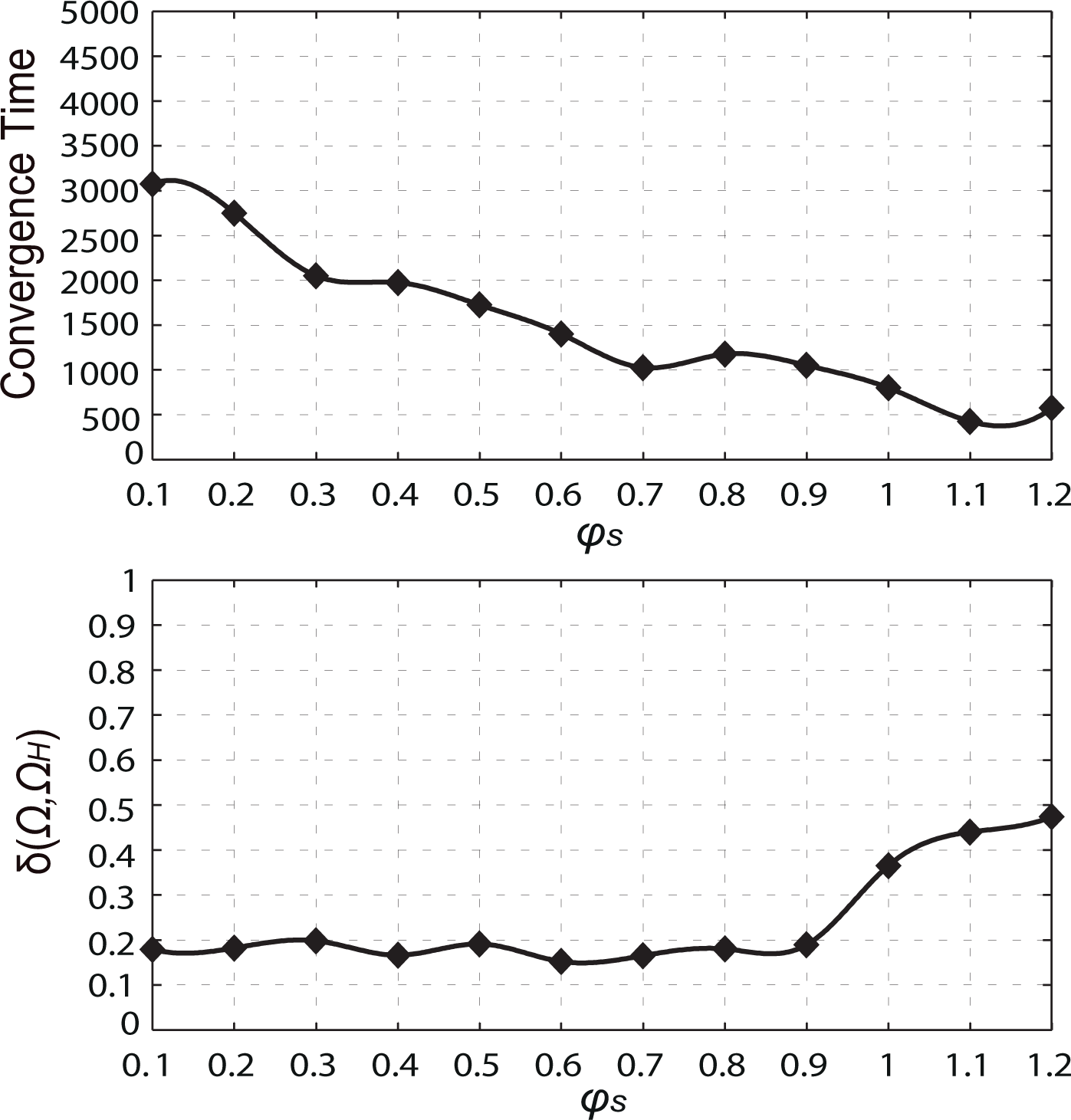
The convergence time and the PCD value δ(Ω,Ω_H) as a function of φ_s when the system first reaches the equilibrium state

As can be seen in Figures 4 and 5, when φ_s increases, S_init increases (the initial node density ρ_init deceases) for a fixed N and the convergence time decreases. When S_init is in the interval of [0.1S_perf, 0.9S_perf], the value of δ(Ω,Ω_H) is small and relatively stable, which indicates the final network topology is approximate to a hexagonal structure and that deployment is successful. When S_init is in the interval of [0.9S_perf,1.2S_perf], the value of δ(Ω,Ω_H) significantly increases. The system converges quickly but the deployment result is not good, which may be caused by a local optimum with a blank monitoring area.

Figure 6.

Typical profiles of PCD δ(Ω,Ω_H) as a function of the time step for the specified values of G

Based on Figure 5, we concluded that when φ_s is in the interval of [0.7,0.9] or when S_init is in the interval of [0.7S_perf,0.9S_perf], both the convergence rate and the deployment structure are relatively good. The corresponding optimal range of the initial node density, ρ_init, is [(1.11ρ_perf, 1.43ρ_perf].

4.3 The Influence of the Exchange Force Constant

From Equations (2) and (4), one can clearly see that the constant G significantly affects the total exchange force that determines the velocity of the node. Here, we discuss in detail the influence of different exchange force G values on the convergence time and the deployment results.

We fixed S_init=0.7S_perf and used the values for Section 4.2 for the other parameters. In Figure 6, we present profiles of the PCD δ(Ω,Ω_H) as a function of the time step for the specified cases of G=0.01,0.02, ⋅⋅⋅, 0.20. When G is small - say G < 0.03 - the system exhibits poor convergence all of the time. However, the convergence time decreases as the value of G increases. When G > 0.18, the sensor distribution ultimately obtains a bad network topology.

In Figure 7, we present the convergence time and the PCD value, δ(Ω,Ω_H), as a function of G using cubic spline interpolation according to the results of Figure 6. The system clearly exhibits a good convergence time when G is in the interval of [0.09,0.19] and when the value of δ(Ω,Ω_H) is small, while it is relatively stable when G is in the interval of [0.01,0.17]. Thus, the optimal range of G is [0.09,0.17] and both the convergence time and the network topology are relatively good.

Figure 7.

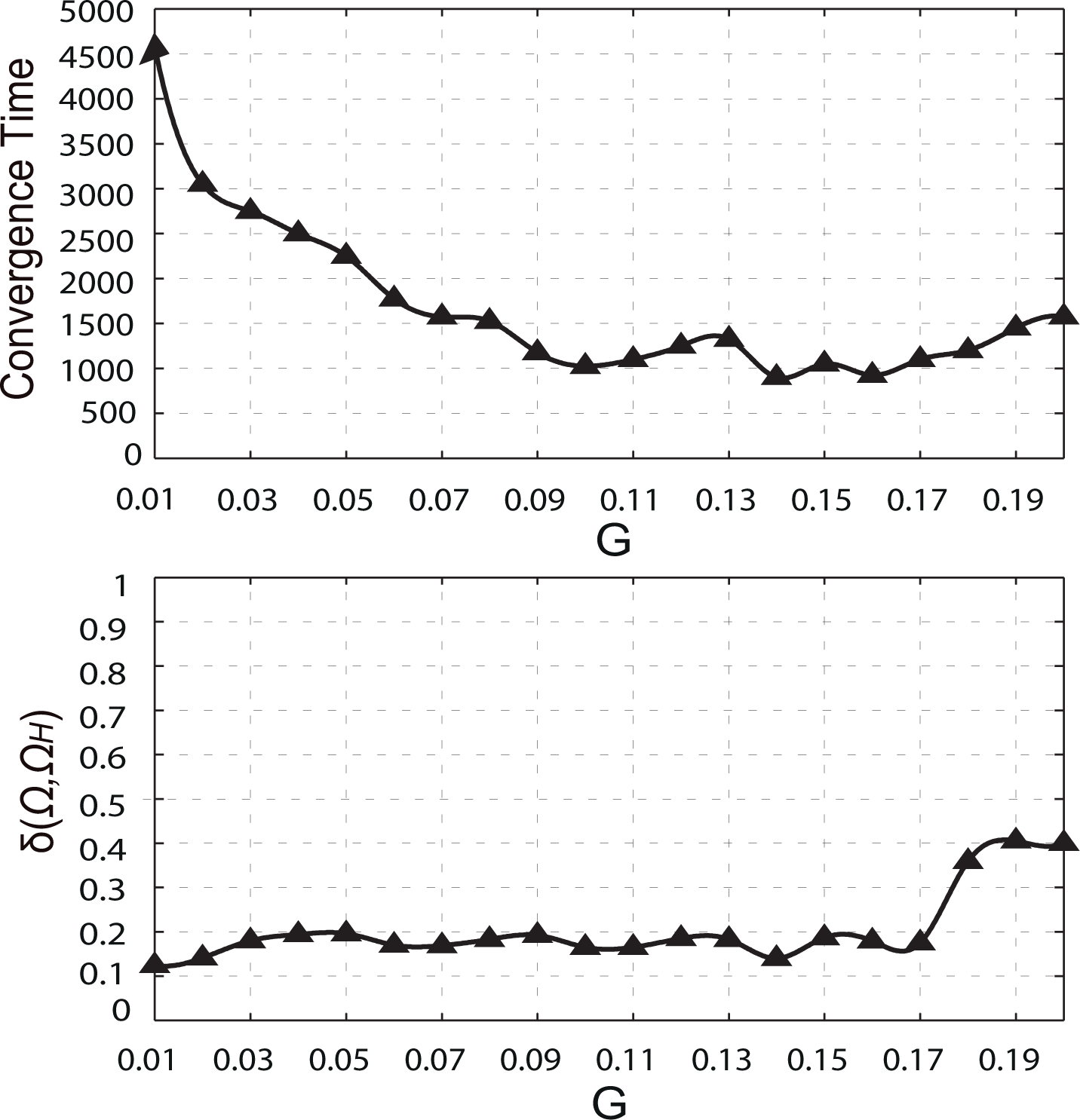
The convergence time and the PCD value δ(Ω,Ω_H) as a function of G when the system first reaches the equilibrium state

Figure 8.

The convergence time and the PCD value for δ(Ω,Ω_H) as a function of G for the specified values of φ_s when the system first reaches the equilibrium state

4.4 Optimal (φs,G)-Parameter Space

Using the convergence time and the PCD δ(Ω,Ω_H) as performance indicators for sensor deployment, we obtained a detailed parameter investigation based on additional simulations and the optimal parameter space of φ_s and G.

Table 1.
The optimal range of G for different φ_s and the average convergence time and $δ (Ω, Ω_{H})$ under an optimal range of G

φ_s Optimal G Convergence Time δ(W,W_H)

0.1 [0.05, 0.10] 3246 0.189

.2 [0.06, 0.10] 2735 0.176

.3 [0.06, 0.15] 2235 0.185

.4 [0.09, 0.15] 1793 0.185

.5 [0.10, 0.15] 1117 0.188

.6 [0.09, 0.16] 1322 0.182

.7 [0.09, 0.17] 1094 0.175

.8 [0.09, 0.13] 860 0.165

.9 [0.11, 0.15] 670 0.177

.0 0.13 500 0.202

φ_s	Optimal G	Convergence Time	δ(W,W_H)
0.1	[0.05, 0.10]	3246	0.189
.2	[0.06, 0.10]	2735	0.176
.3	[0.06, 0.15]	2235	0.185
.4	[0.09, 0.15]	1793	0.185
.5	[0.10, 0.15]	1117	0.188
.6	[0.09, 0.16]	1322	0.182
.7	[0.09, 0.17]	1094	0.175
.8	[0.09, 0.13]	860	0.165
.9	[0.11, 0.15]	670	0.177
.0	0.13	500	0.202

Similar to the previous figures, in Figure 8 we plot the convergence time and the PCD value δ(Ω,Ω_H) as a function of G for the specified cases φ_s=0.1,0.2, ⋅⋅⋅, 1.0 when the system first reaches the equilibrium state. Table 1 provides the optimal range of G for which both the convergence rate and the deployment results are relatively good for different φ_s. We also provide the average δ(Ω,Ω_H) and the convergence time under the optimal range of G.

According to the data in Table 1, as shown in Figure 9, we draw a relationship diagram between φ_s and the optimal ranges of G. The green curve displays the average convergence time under the optimal range of G for different φ_s, and decreases as φ_s increases. The red curve displays the PCD value δ(Ω,Ω_H) under this optimal range of G, which is relatively small. In general, sensor deployment requires a short convergence time in order to obtain a quick response for emergent situations and energy saving. In our simulations, when the convergence time is in the interval [500,1500], the system has the best performance. The purple shadow in Figure 9 shows areas of good (φs,G)-parameter space.

Figure 9.

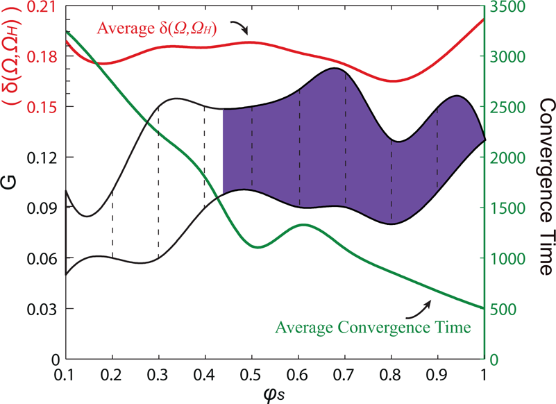
A relationship diagram between φ_s and the optimal ranges of G

5. Conclusion

In this study, we introduced an optimized virtual force algorithm based on the exchange force, in which a new shielding rule based on a Delaunay triangulation which accurately defines adjacent nodes was adopted. We also used a new performance metric called ‘pair-correlation diversion’ to evaluate the uniformity of the distribution. Simulation results verified the effectiveness of the algorithm. We also provided a detailed discussion of the parameter effect and obtained an optimal region for the (φ_s,G)-parameter space. Our results have implications for choosing input parameters in actual experiments and also for the analysis of sensor data in robotics systems. In our future work, we will attempt to enlarge the shielding range and compare the shielding effects in different physical systems (e.g., a dusty plasma system).

Footnotes

6.

Our work was supported by the National Science Foundation of China (Grant No. 41464007), the Science Foundation of Jiangxi Province (Grant No. 2014BAB202008), the Specialized Research Fund for the Doctoral Program of Higher Education (Grant No. 20133601120005); and the Educational Foundation of Jiangxi Province (GJJ13050).

References

Akyildiz

I. F.

Sankarasubramaniam

, and Cayirci

(2002) Wireless sensor networks: a survey. Computer Networks, 38(4): 393–422.

, and Yang

(2006) A survey on topology issues in wireless sensor network. In: International Conference on Wireless Networks, p. 503.

Wang

Cao

, and La Porta

(2006) Movement-assisted sensor deployment. IEEE Transactions on Mobile Computing, 5(6): 640–652.

Takahara

, and Hassanein

(2006) On the robustness of grid-based deployment in wireless sensor networks. In: Proceedings of the 2006 International Conference on Wireless Communications and Mobile Computing, ACM, p. 1183–1188.

Guo

X. M.

Zhao

C. J.

Yang

X. T.

Sun

, and Zhou

(2012) A deterministic sensor node deployment method with target coverage based on grid scan. Chinese Journal of Sensors and Actuators, 25(1): 104–109.

Howard

Matarić

M. J.

, and Sukhatme

G. S.

(2002) Mobile sensor network deployment using potential fields: a distributed, scalable solution to the area coverage problem. In: Proceedings of the 6th International Symposium on Distributed Autonomous Robotics Systems 5, p. 299–308.

Zou

, and Chakrabarty

(2003) Sensor deployment and target localization based on virtual forces. Proceedings of the 22nd Annual Joint Conference of the IEEE Computer and Communications, 2: 1293–1303.

Heo

, and Varshney

P. K.

(2003) A distributed self-spreading algorithm for mobile wireless sensor networks. In: WCNC, 3:1597–1602.

Kribi

Minet

, and Laouiti

(2009) Redeploying mobile wireless sensor networks with virtual forces. In: Wireless Days, IEEE 2nd IFIP, p. 1–6.

10.

Garetto

Gribaudo

Chiasserini

C. F.

, and Leonardi

(2007) A distributed sensor relocation scheme for environmental control. IEEE International Conference on Mobile Adhoc and Sensor Systems, p. 1–10.

11.

Huang

Lan

, and Qian

(2012) A novel virtual force aproach for node deployment in wireless sensor network. In: Proceedings of the IEEE 8th International Conference on Distributed Computing in Sensor Systems, p. 359–363.

12.

Liu

Huang

Qian

, and Zhang

(2013) A node deployment algorithm based on van der Waals force in wireless sensor networks. International Journal of Distributed Sensor Networks, Volume 2013, Article ID 505710, 8 pages, doi: 10.1155/2013/505710.

13.

Yang

Lian

, and Li

(2013) Deploying three-dimensional mobile sensor networks based on virtual forces algorithm. In: Advances in Wireless Sensor Networks, Springer Berlin Heidelberg p. 204–216

14.

Liu

Qian

, and Zhang

(2014) A deployment method based on spring force in wireless robot sensor networks. International Journal of Advanced Robotic Systems, 11: 79.

15.

Wen

Qian

Song

, and Bartos

(2014) On virtual-force algorithms for coverage-optimal node deployment in mobile sensor networks. Unpublished work.

16.

, and Lei

(2009) Sensor node deployment in wireless sensor networks based on improved particle swarm optimization. International Conference on Aplied Superconductivity and Electromagnetic Devices, p. 215–217.

17.

Kukunuru

Thella

B. R.

, and Davuluri

R. L.

(2010) Sensor deployment using particle swarm optimization. International Journal of Engineering Science and Technology, 2(10): 5395–5401.

18.

Liao

W. H.

Kao

, and Li

Y. S.

(2011) A sensor deployment aproach using glowworm swarm optimization algorithm in wireless sensor networks. Expert Systems with Aplications, 38(10): 12180–12188.

19.

Huang

Zhang

Wang

, and Qian

(2014) Sensor node deployment in wireless sensor networks based on ionic bond-directed particle swarm optimization. Aplied Mathematics and Information Sciences, 8(2): 597–605.

20.

Suen

(2004) A genetic-algorithm based mobile sensor network deployment algorithm. Technical report, Department of Electrical and Computer Engineering, The University of Texas at Austin.

21.

Öztürk

Karaboga

, and Görkemli

(2012) Artificial bee colony algorithm for dynamic deployment of wireless sensor networks. Turkish Journal of Electrical Engineering and Computer Sciences, 20(2): 255–262.

22.

Zhang

Fan

, and Zhang

(2013) A faster convergence artificial bee colony algorithm in sensor deployment for wireless sensor networks. International Journal of Distributed Sensor Networks, Volume 2013, Article ID 497264, 9 pages, doi: 10.1155/2013/497264.

23.

Wang

Liao

, and Hu

(2012) Wireless sensor network deployment using an optimized artificial fish swarm algorithm. International Conference on Computer Science and Electronics Engineering, 2: 90–94.

24.

Lin

F. Y.

, and Chiu

P. L.

(2005) A near-optimal sensor placement algorithm to achieve complete coverage-discrimination in sensor networks. IEEE Communications Letters, 9(1): 43–45.

25.

Wang

, and Ma

J. J.

(2007) An improved co-evolutionary particle swarm optimization for wireless sensor networks with dynamic deployment. Sensors, 7(3): 354–370.

26.

Han

Y. PL

Kim

Y. H.

Kim

, and Jeong

Y. S.

(2012) An energy-efficient self-deployment with the centroid-directed virtual force in mobile sensor networks. Simulation, 88(10): 1152–1165.

27.

O'Rourke

(1998) Computational geometry in C. Cambridge University Press.

28.

Quinn

R. A.

Cui

Goree

Pieper

J. B.

Thomas

, and Morfill

G. E.

(1996) Structural analysis of a Coulomb lattice in a dusty plasma. Physical Review E, 53(3): 2049–2052.

29.

Hua

Liu

Wang

and Zhang

(2003) Structural and dynamical analysis of a two-dimensional dusty plasma lattice. Chinese Physics Letters, 20(1): 155.

30.

Liu

, and Snoeyink

(2005) A comparison of five implementations of 3D Delaunay tessellation. Combinatorial and Computational Geometry, 52: 439–458.

Optimized Node Deployment Algorithm and Parameter Investigation in a Mobile Sensor Network for Robotic Systems

Abstract

Keywords

1. Introduction

2. The Optimized Node Deployment Algorithm

2.1 Review of the VFA

4. Simulation Results and Discussion

4.1 Effectiveness Verification

Footnotes

6.

References