Sage Journals: Discover world-class research

Abstract

Equipped with micro wireless sensor nodes, a unmanned aerial vehicle) cluster can form an emergency communication network, which can have several applications such as environmental monitoring, disaster relief, military operations and so on. However, situations where there is excessive aggregation and small amount of dispersion of the unmanned aerial vehicle cluster may occur when the network is formed. To mitigate these, a solution based on a 3D virtual force driven by self-adaptive deployment (named as 3DVFSD) is proposed. As a result, the three virtual forces of central gravity, uniform force, and boundary constraint force are combined to act on each node of the communication network. By coordinating the distance between the nodes, especially the threshold of the distance between the boundary node and the boundary, the centralized nodes can be relatively dispersed. Meanwhile, the nodes can be prevented from being too scattered by constraining the distance from the boundary node to the end. The simulation results show that the 3DVFSD algorithm is superior to the traditional virtual force-driven deployment strategy in terms of convergence speed, coverage, and uniformity.

Keywords

Wireless sensor node micro-unmanned aerial vehicle (MUAV)three-dimensional deployment virtual force algorithm emergency communication network

Introduction

With the rapid development of communication and embedded computing technologies, a variety of micro sensors that can be used for sensing, computing and communicating have been developed. Wireless sensor networks (WSNs) equipped with micro-sensor nodes have been widely employed in environmental monitoring, military applications, territorial security, disaster relief, and so on.¹ WSNs are capable of real-time collaborative monitoring, perception, collection of specific information within the coverage area, and the online processing of this data in harsh environments that are not easily accessible for humans. This paper proposes to construct an emergency communication network formed by the UAV cluster equipped with wireless sensors when the fixed communicating infrastructure was seriously damaged, or even completely destroyed. Each node in the network works as a cooperative communication relay, lots of nodes dynamically build up a network to provide network communication services in damage detection and rescue missions.

Specifically, with respect to the construction of UAV networks, this paper focuses on the self-adaptive deployment model of the UAV cluster. The UAVs are equipped with wireless sensor nodes capable of sensing and communication, and they have small size and robust mobility. Aided by the large aircraft platform, can easily realize long-distance delivery, shedding, and the UAVs can self-adaptively cover the disaster-affected area in optimal topological structure. The advantages of the emergency communication network include low cost, robust mobility, and independent construction, and do not require the construction of any communicating infrastructure, and so on. Even several UAVs are disabled for limited energy or mechanical failure, all the left UAVs can self-adaptively move according to special deployment model. Thus, communication can be facilitated and the data required for rescue operations decisions can be provided from dangerous areas where humans cannot reach.

During the process of dynamically self-adaptive deployment, some MUAV nodes often encounter the problem of escape of the MUAV nodes² and excessive aggregation, leading the WSN does not cover the target region fully. In order to solve the problem mentioned above in emergency situations, and depending on one self-adaptive strategy to realize that the MUAV nodes can uniformly fill up the target region, which is regular or irregular 3D space, this paper proposes an algorithm based on a three-dimensional (3D) virtual force driven by self-adaptive deployment. Based on the conventional virtual force method, the central gravity (CG), uniform force (EF) and border constraint force (BCF) are integrated at each UAV node. At the same time, to disperse the relatively clustered nodes, thresholds are introduced for the distance between the nodes, while the threshold of the distance between the boundary nodes and the end are introduced to realize uniform coverage of the key regions. In addition, when facing complex target areas, the concept of the adaptive central aggregation force is introduced so that the sensor network can cover the surface of complex objects in 3D space better.

Related works

The deployment of wireless sensor networks can be divided into two types, the static deterministic deployment and dynamic self-organizing deployment. It is difficult to successfully employ deterministic deployment strategies in unknown or harsh environments. The self-organizing deployment method can scatter the nodes randomly and achieve the goal of uniform coverage of the region of interest using the self-organizing deployment algorithm. In recent years, researchers have studied 3D networks extensively although most of the work has been limited to 3D static deployment.

Considering mobile self-organizing deployment, the successful formation of a relatively stable sensor-equipped UAV topology in the high-altitude environment remains a problem. The UAV may possibly deviate from the target area with a possibility of escape, or the nodes may be too concentrated. The two cases mentioned above both induce coverage loopholes and not satisfied full coverage toward target area. To address these issues, this paper proposes to mitigate the problem of target coverage in 3D space by formulating a constraint strategy to ensure that the nodes of the 3D UAV automatically form a reasonable distribution in the target space. This work extends the work in Tzamaloukas and Garcia-Luna-Aceves³ from 2D space to 3D space. Kelvin’s conjecture⁴ and Kepler’s conjecture⁵ indicate the complexity of the problem. Li et al.⁶ contains a landmark study on the problem of ball stacking and covering and proposes the use of Voronoi’s element space mosaic theory to formulate different node placement strategies. Wang et al.⁷ and Zhu et al.⁸ propose a similar strategy to gain good adaptability with respect to changes of the number of sensor nodes and the size of the monitoring area, but in 3D space its performance is severely limited. Although Wang et al.⁹ and Zhu et al.¹⁰ take the 3D space scenario into account, and obtain a certain degree of improvement in coverage speed, their strategy’s main drawbacks lies in low coverage rate toward the border region, and these two different static polices constraint on growth of coverage speed. Wang et al.⁹ focuses on meteorological sensing scene. Shi et al.^11–13 notice the coverage problem toward border 3D region, they all adopt probability strategy, to make the mobile nodes on the edge of the target zone keep moving in any direction with a certain probability. This strategy obtains good performance in coverage rate but its network convergence rate is poor, especially these nodes on border, so this type of strategy is not widely used in practice due to its low coverage efficiency. All the references mentioned above do not consider how to efficiently deploy nodes under the complex geographical conditions. Although Zheng et al.¹⁴ take the complex geographical conditions into account, the complex region is regular geometrical shape, so its algorithm is not with a wide range application and adaptability. In summary, there has been scarcely dissertations to research the deployment under the complex irregular condition.

The study is based on the following assumptions:

The binary disk sensing model is adopted. When the target event is within the sensing radius of the sensor, the probability of detection remains 1. Otherwise, it is 0.

The detected target area is always static or slow-moving. As a result, it can always stay in the perception range of the network. Along with the strong Doppler effect, the state of non-convergence of the network owing to the fast-moving objects that may cause sensor nodes to constantly adjust their position also needs to be considered in the communication process

It is assumed that the target position has been perceived by nodes in the initial state because path planning and target area location are beyond the scope of this paper. In addition, sensor data fusion, underlying protocol communication, and other issues are not included in the discussion of this paper.

Algorithm description

Introduction of 3D virtual force model

The basic VFA (virtual force algorithm)¹⁵ considers that there is mutual attraction and repulsion between the nodes, and that they form a close structure under the synergistic effect. When the node stays in the communicating range, attraction is used to gather the node. On one hand, the larger the distance, the greater the attraction. On the other hand, when the nodes are too close, the coverage areas of multiple nodes will overlap and the repulsive force will increase, and then, the repulsive force can be used to avoid node collisions. The 3D virtual force model mentioned in the paper makes the node group stable and compact by using the resultant force of attraction and repulsion. The direction of the resultant force determines the direction of motion of the node at the next moment.

The authors extended the work described in Cohen et al.,¹⁶ which defined the node model in a two-dimensional space, to suit a 3D space so that each node can correspond to three concentric spheres:

Perception sphere: Each node can sense the target events omnidirectionally within the radius R_s. The spherical region formed in this way is called the perception sphere;

Communication sphere: Each node can communicate directly to neighbor nodes within the radius of R_c through wireless channels. The corresponding communication area is defined as the communication sphere;

Balanced sphere: The sphere formed by the radius R_b (0 ≤ R_b ≤ R_c) is the boundary between attraction and repulsion. Each sensor node has only a repulsion effect on the neighbor node with a radius less than R_b and only an attractive effect on the other neighbor nodes.

In the 3D virtual force system, each node is assumed to be self-centered and can generate a potential field, which exerts different effects on its neighbor nodes. Figure 1 shows an example considering B1 as the reference point. The communication ball, balanced ball and perception ball generated by B1 are represented by the yellow, green, and blue colors, respectively. Among them, the B2 node inside the B1 balance ball is repulsed by B1, B3 node outside the B1 balance ball is attracted by B1, and B4 node on the B1 balance ball is in a state of force balance, without any virtual force from B1. In addition, B5 is not even a neighbor of B1 because it remains outside the communication sphere of B1, and so, it is not affected by the B1 potential field. Due to the mutual forces, B1 is also in the potential field of its neighbor nodes and subject to the repulsive force (attraction) from B2 (B3). At the end of each cycle of the algorithm, the virtual force relationship between the nodes and different neighbor nodes is calculated, and their vector sum is obtained so as to determine the direction of motion in 3D space at the next moment.

Figure 1.

Virtual force field of node B1.

3D virtual force algorithm

According to the virtual force rules,¹⁷ the closer or farther the distance between any two nodes is, the greater the repulsive force or attractive force generated by each other. Any model with these characteristics can be used to calculate the virtual force.

First, define the node model based on virtual force.

Definition 1

The node model can be represented by a six-tuple < S, R, v, n_s, F, f >, here S(x, y, z) represents the coordinates of the node. R ={Rs, Rb, Rc} is the radius attribute set of the node itself, that is, the generated radius of the three concentric spheres. The term v represents the node speed in 3D space, f is a binary variable, 1 means that the node is within the target area, and if it is not, the value is set as −1. If the distance between two nodes is less than Rc, they are called neighbor nodes. Js represents the set of neighbor nodes of node s, and this may be represented by

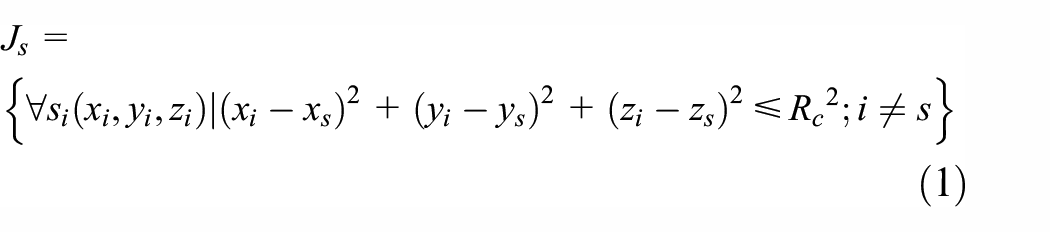
\begin{array}{l} J_{s} = \\ {\forall s_{i} (x_{i}, y_{i}, z_{i}) | {(x_{i} - x_{s})}^{2} + {(y_{i} - y_{s})}^{2} + {(z_{i} - z_{s})}^{2} \leq {R_{c}}^{2}; i \neq s} \end{array}

(1)

F ={TV, CG, EF} is the set of force fields generated by node S. Detailed descriptions and definitions of the three forces will be given later.

Definition 2

For any two sensor nodes S₁(x₁, y₁, z₁) and S₂(x₂, y₂, z₂) in the communication range in 3D space, the Euclidean distance is:

d (s_{1}, s_{2}) = \sqrt{{(x_{1} - x_{2})}^{2} + {(y_{1} - y_{2})}^{2} + {(z_{1} - z_{2})}^{2}}

(2)

Let the traditional virtual force (TVF) applied by S₁ to S₂ be $\vec{TV F_{12}}$ , the direction of the vector is determined by the type of virtual force, and the magnitude may be calculated by formula (3)

| \vec{TV F_{12}} | = ((d (s_{1}, s_{2}) - R_{b}) \times α)^{k}

(3)

Among them, k represents the magnification index, which may be used to magnify the influence of the distance from the equilibrium point. The term α (assigned value of 10) is used to ensure that the equation is an increasing function. The virtual force calculated by formula (3) makes the adjacent nodes move toward the surface of the balance ball. Each sensor node automatically adjusts its current position by comprehensively calculating the positional relationship with the neighbor nodes in 3D space, thereby generating a highly coupled network structure. By adjusting Rb, the overall deployment can be made relatively loose or compact.

The traditional virtual force algorithm usually assumes that the initial distribution of the node group is relatively dense,¹⁸ and the network is uniformly deployed through diffusion. However, in practical applications, the nodes are usually randomly scattered in a 3D space and move to find the target area. The traditional virtual force algorithm implemented on this basis usually causes network segmentation or coverage loopholes, and further adjustments are needed to make dense areas sparser or sparse areas more compact. The traditional virtual force algorithm does not perform well in this case, because the statuses of the nodes are equal and prior knowledge is limited. The coverage density of other individual areas are not known, and so, they can only use local rather than global information to make decisions.

The lack of overall coordination brings about two potential problems. First, the target area may not be well covered. Random positioning and self-adaptive deployment methods without external interference may result in large or small offsets to the target. Second, even if the previous problem is solved, the nodes may eventually be deployed unevenly. In extreme cases, even if the network is in a balanced state under the action of the virtual forces, there may still be multiple network partitions locally. In addition to the traditional virtual force TVF, this chapter defines the central gravity CG, uniform force EF, and boundary constraint force BCF, making the deployment process more reasonable and effective.

Definition 3

CG is defined as the positive attraction of the target area to the node group. For details, please refer to the traditional potential field method, such as the Euclidean distance correlation function. The 3DVFSD algorithm defines CG as a constant of the same magnitude as TVF.

The sensor nodes in the 3D space move randomly to search for the target area. Once the target is confirmed, the sensor node will move in the direction of CG generated by the target, and at the same time it will notify other companions of the coordinate position of the target. In this way, the node group is attracted to the target area through CG.

On the other hand, the distributed deployment strategy is a non-central control algorithm. Due to the limitations of individual knowledge, the tightly coupled structure formed only by TV is likely to contain regions with uneven density. However, this uniform distribution is of great practical significance. A well-ordered formation can make full use of the effective coverage area of each node, thereby greatly reducing the number of mobile nodes.

The most effective distribution method must be based on a deterministic deployment strategy, such as a truncated dodecahedron model. However, the self-deployment shape based on virtual force is unpredictable. According to the Voronoi polyhedron model,¹⁹ the destination position of each node is dynamically calculated, and the node is moved to this coordinate; regardless of the high computational cost of the system, the operability not too high as this is not strictly an adaptive strategy in nature. The best solution should be based on a complete distribution criterion that satisfies the actual situation. Here, the concept of uniform force EF is proposed.

During the deployment process, each node not only acts as a potential field for generating TVF, but also as a coordinator to balance the self-centered local area through EF. For simplicity, Euclidean distance is used for the calculation. Each node calculates the average distance between all its neighbor nodes, and then compares this value with individual neighbors. If the average value is greater than the individual value, a repulsive force is generated; otherwise, an attractive force is generated.

Definition 4

Taking node i as a reference, the uniform force that it produces on neighboring node j is $\vec{E F_{ij}}$ , and the magnitude is defined by formula (4)

| \vec{E F_{ij}} | = ((d (s_{i}, s_{j}) - \bar{D_{i}}) * α)^{k}

(4)

Among them, $\bar{D_{i}}$ represents the average value of the distance from node i to all its neighbor nodes. The terms α and k are as defined earlier.

Definition 5. Taking the node i as a reference, the boundary restraint force $\vec{BC F_{i}}$ is generated by the boundary on the neighbor node i, and the magnitude of the force is

\begin{matrix} | \vec{BC F_{i}} | = \frac{2 S}{\sum_{i \in G} (f_{i} + 1) \cdot π \cdot R)^{2}} \\ ((\min {d (s_{i}, B)} - R_{th}) \times α)^{k} \end{matrix}

(5)

Among them, R_b represents the average of the distances from node i to all its neighbor nodes. When R = R_c, the network mainly exists as a pure communication network; when R = R_s, the communication network can collect data also. The quantity min{d(s_i,B)} represents the shortest distance between node i and the boundary of the deployment area. The parameter R_th serves as the boundary distance threshold between the gravitational and repulsive forces. The region boundary only produces repulsive force on the neighbor nodes within R_th from the region boundary, and only gravitational force on neighbor nodes within [R_th, 2R_th]. Then, the parameters α and k in formula (5) are the same as those in formula (2).

Def. 6. The direction of the resultant force $\vec{F_{i}}$ determines the moving direction of node i in the next time step. It is defined as follows

\vec{F_{i}} = \vec{CG} + \vec{BC F_{i}} + \sum_{j = 1}^{N_{i}} (\vec{TV F_{ij}} + \vec{E F_{ij}})

(6)

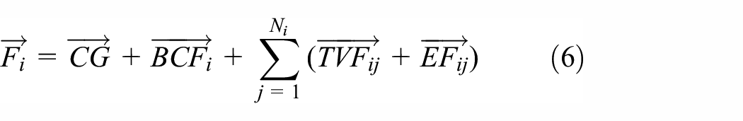
where N_j represents the neighbor nodes set of node i.

At each time step, CG is calculated based on the distance between the node and the target area, BCF is calculated based on the distance relationship between the node and the boundary, TVF and EF are calculated based on the relationship between the node and its neighbor nodes, and then all the virtual force vectors are calculated and summed to obtain a joint force. In this way, each node adjusts its position under the driving force of the resultant force until its force balance stops. When each node reaches the force balance, it also means that the entire network is in a stable topological state, and can perform sensing tasks on the target area covered by it.

3DVFSD algorithm description

The 3D virtual force driven by the self-adaptive deployment algorithm is used as a distributed algorithm. Each sample node executes the same strategy concurrently, and the position adjustment is performed simultaneously. The location update algorithm description of any node is shown in Figure 2.

Figure 2.

3DVFSD algorithm description.

From Figure 2 we can see that first each node must know its own location and the target location by itself or through others notifying, then according to the virtual force vector calculated by 3DVFSD algorithm to update its own moving direction. The process will end util the network convergence finishes, that is, each node suffered force is zero. Meanwhile, we can easily calculate the time complexity of 3DVFSD algorithm is O(nlogn), and the time complexity of traditional VFA is O(n²). Obviously, 3DVFSD is better than traditional VFA in terms of time complexity. The time complexity of this algorithm is low, and it live up to the especial request in response time.

Simulation experiment

A simulation experiment was carried out in a 3D scene, and coverage and uniformity were the two experimental indexes. The former determines whether the node effectively covers the target area, and the latter focuses on quantifying the distance between the nodes, which is used to measure whether the node is evenly distributed. Considering only the 1-coverage, in contrast to the deterministic deployment strategy, the initial distribution state of the network nodes for mobile adaptive deployment is unknown, and may be relatively clustered or relatively scattered, or both. This is why a uniformity evaluation standard is required. And we choose the traditional VFA (virtual force algorithm) as the unique comparison object, for two reasons, one is that traditional VFA as the classic algorithm, the other is that few researches focus on deployment under complex irregular condition. For the foregoing reason, we choose VFA as the unique comparison object.

Experimental settings

The simulation experiment was carried out on the Matlab2011b platform. Based on the premise of a homogeneous network and considering the uncertain influence of the aerodynamic conditions in the air, the nodes are randomly scattered in the target airspace and have the same sensing radius and communication radius. Main experimental parameters are described in the Table 1, and the initial values of these experimental parameters refer to settings widely accepted in the field of self-adaptive deployment.¹⁹

Table 1.

Main experimental parameters.

Name	Definition
Rs	Sensing radius;
Rc	Communication radius;
R_th	Distance threshold between gravitational and repulsive forces
D_ij	Distance between S_i and S_j;
<S, R, v, n_s, F, f>	S(x, y,z) represents the coordinates; R ={Rs, Rb, Rc} is the radius attribute set; v represents the node speed; f is a binary variable;
k_min	Safety distance;

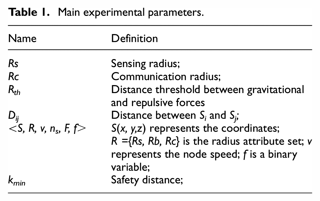
Let Rs be 1 and Rc be 3. In addition, by comprehensively comparing the data obtained from multiple simulation experiments and combining with the Van Der Wals Force^15,20,21 the parameters are RTH = 2.3, RB = 1.4, and k = 12 in formula (3) and formula (4) when the deployment is relatively ideal.

R{(x₁, x₂), (y₁, y₂), (z₁, z₂)} represents the 3D space within the coordinate range of x₁≦x≦x₂, y₁≦y≦y₂, z₁≦z≦z₂. R{(–5,5), (–5,5), (–5,5)} represents the largest initial state 3D region scattered by MUAV. O(0, 0, 0) is the origin. To verify the effectiveness of the algorithm, two comparative test schemes are proposed. The specific settings are as follows:

The initial area of the randomly scattered MUAV is R₁{(–0.5,0.5), (–0.5,0.5), (–0.5,0.5)}, as shown in Figure 3(a). This scheme investigates how MUAV can adaptively diffuse and uniformly deploy when the initial state distribution is relatively concentrated.

R ₂{(–5,5), (–5,5), (–5,5)} is the 3D area of the initial state distribution of MUAV which in the worst case, as shown in the Figure 4(a). This scheme mainly verifies how MUAV works when the initial distribution of MUAV is relatively scattered.

Figure 3.

Unfolding process of 3DVFSD in initial state of aggregation.

Figure 4.

Unfolding process of 3DVFSD in initial state of dispersion.

These two configurations summarize the application requirements of different deployment processes in 3D space. Figures 3 and 4 show the detailed deployment process of each scheme based on the time node when the node scale reaches 60. The sphere in the figure represents the perception range of the MUAV node. It can be seen from the figure that the deployment effect is extremely obvious, and the MUAV group can finally achieve a state of uniform coverage with tight deployment. Next, select the network scale of 100 nodes for the simulation experiment, run the traditional and the improved VFA independently for 10 iterations, and then compare and analyze the arithmetic average of the calculated evaluation index parameters. Among them, the traditional virtual force algorithm involved in the figure comes from the extension of the basic virtual force algorithm in the 3D space given in Tang et al.¹⁹

Coverage calculation

The methods for calculating the coverage rate are often complex. The Monte Carlo method²⁰ is used for continuous random sampling of points in the target area and calculating the ratio of the coverage area that meets the requirements of the constraint conditions. In each calculation cycle, the number of points considered is large enough to enhance the calculation accuracy.

Experiments show that under the existing parameter configuration conditions, the three additional virtual constraint conditions of the virtual force algorithm cover a portion of 3D space represented by R’{(2.5, 2.5), (2.5, 2.5), (2.5, 2.5)}. While the traditional virtual force algorithm based on the 3D space extension only considers the gravitational and repulsive forces, the maximum coverage space is only R’{(–2.12,2.12), (–2.12,2.12), (–2.12,2.12)}. So the experiment takes R’ as the target area to compare the algorithm performance. At the same time, the entire space R*{(–5,5), (–5,5), (–5,5)} is considered for the comparison. Figure 5 shows the statistical results under different configurations. Obviously, the improved virtual force algorithm can reach the full coverage requirement of the R’ area at an earlier time, while the traditional virtual force algorithm is still in a state of constant adjustment. This is because the existence of the uniform force EF and the boundary constraint force BCF can constantly adjust the areas to make dense areas sparser and vice versa, so as to more efficaciously use the effective coverage area of the sensor node, and furthermore, it is easier to make the improved virtual force algorithm reach the 1-cover state.

Figure 5.

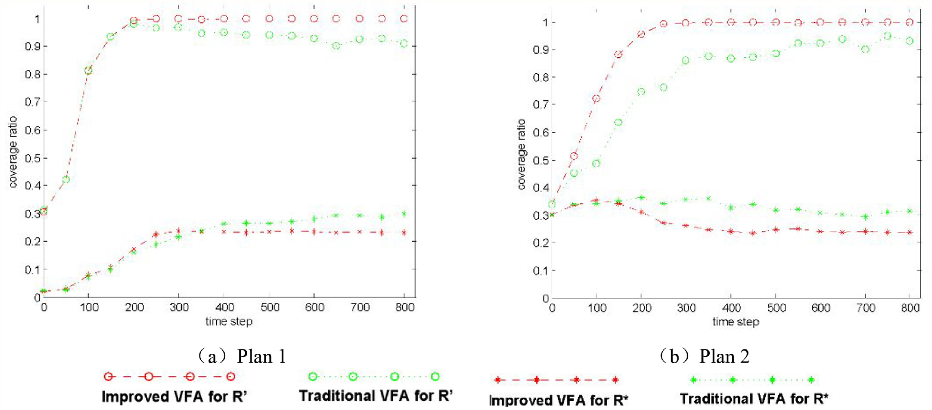
Coverage rate.

In addition, due to the insufficient coverage of the traditional virtual force algorithm in the area ’, so more loose parts are generated outside R’, so that for the whole space R*, the traditional virtual force algorithm will eventually have a higher coverage rate, which is also fully reflected in Figure 5.

Uniformity calculation

The degree of homogeneity or homogeneous degree (HD) is represented by the arithmetic mean of local uniformity, and each local uniformity is calculated from the variance of the standard distance between a node and its neighbors. The calculation formula is as follows

HD = \frac{1}{n} \sum_{i = 1}^{n} \sqrt{\frac{1}{N_{i}} \sum_{j = 1}^{J_{i}} {(d_{ij} - \bar{D_{i}})}^{2}}

(7)

where D_ij represents the Euclidean distance between node S_i(i = 1 … n) and S_j(j = 1 … m), and it is the average value of the distance between node Si and all the adjacent points.

The lower the uniformity, the better the consistency and uniformity of the sensor node distribution. Figure 6 describes the comparison of uniformity changes in different cases. The uniformity of the improved virtual force algorithm can reach a relatively stable state earlier, while the uniformity of the traditional virtual force is constantly oscillating. The variation rule of uniformity in the figure is essentially caused by the influence of EF and BCF. During the deployment process, the existence of EF and BCF causes the sensor nodes to be attentive to the problem of local consistency and adaptively modulate the influence of TVF. Without a uniform force and boundary constraint force, the traditional virtual force algorithm cannot reach a relatively stable state easily.

Figure 6.

Uniformity.

Complex target coverage

In the above experiments, the sensor networks are all deployed in 3D space, forming a pellet. In practice, the network needs to be deployed on the surface of the complex spatial curved surface to monitor and perceive the target area. To avoid node collision, it is necessary to define an additional repulsive force so that the node and the surface of the target area always maintain a safe distance. When a node moves closer to the target, the closest node is called the repulsion origin.²² The repulsive force $F_{t}$ is node t formed on target which keep node t away from the target surface. $F_{t}$ is defined as follows

F_{t} = {\begin{matrix} + \infty & d \leq k_{\min} \\ {(\frac{α}{d})}^{β} & k_{\min} < d \leq Rs \\ 0 & d > Rs \end{matrix}

(8)

Among them, k_min represents the safety distance. After the repulsive origin enters the sensing range of the node, the repulsive force increases with the less distance. When reduced to less than a safe distance, the repulsive force becomes infinite. Figure 7 shows the deployment results obtained from the cone simulation experiment. After 60 air nodes found the cone target, they approached the cone by the central gravitational force at the center of the cone and spread out under the action of the virtual force between them.

Figure 7.

Cone cover.

The top view of the cone in Figure 7 shows that although the nodes are more evenly dispersed in the 3D plane, a large empty area is formed at the top of the cone. The reason for this problem is that the selected central gravitational point is too low, and the corresponding solution is to set the CG point higher. But when facing a non-regular target, it is not easy to select a suitable central gravitational point. Especially, in the case of completely irregular graphics, a particular point may not achieve the desired effect (shown as Figure 8).

Figure 8.

Improved cone coverage.

To solve the problem that the CG point is not suitable or difficult to choose, the adaptive CG strategy is introduced. In the next experiment, a saddle with a more complex spatial structure is selected. Just as in the case of the conical geometry, the adaptive CG is introduced. The side and overlook effects of the deployment process are shown in Figure 9(a)–(d). Sixty nodes are distributed evenly on the saddle surface. The strategy of adaptive CG has played a more obvious role.

Figure 9.

Coverage process on saddle surface.

Conclusion

When constructing an emergency communication network composed of a UAV cluster, it is necessary to automatically deal with the deviation or excessive concentration of the aircraft nodes, to achieve uniform coverage in the target area. Considering that the nodes can move freely in 3D space and the distributed attribute of the virtual force algorithm, this paper proposes and realizes a driven self-adaptive deployment algorithm based on a 3D virtual force, which beneficially extends the traditional virtual force algorithm and introduces CG, Equilibrium Force, and BCF. The simulation results show that the network convergence velocity, coverage rate and uniformity of 3DVFSD are superior to the traditional virtual force-driven deployment strategy, and it can more quickly complete the uniform deployment task in the 3D target area and ensure network connectivity. Therefore, this deployment strategy has strong applicability and shows more reasonable and effective simulation results in different experimental scenarios.

Footnotes

Handling Editor: Lyudmila Mihaylova

Declaration of conflicting interests

The author(s) declared no potential conflicts of interest with respect to the research, authorship, and/or publication of this article.

Funding

The author(s) disclosed receipt of the following financial support for the research, authorship, and/or publication of this article: This work is partially supported by NSFC under Grand (No.U19B2020, No.62162002 and No.61772074); Scientific and Technological Project of HeNan Province (No.182102210486); Key Research Project of HeNan Colleges and Universities (No. 18A520008, No.21A520037).

ORCID iD

Bin Cheng

References

Al-Hourani

Kandeepan

Lardner

. Optimal LAP altitude for maximum coverage. IEEE Wirel Commun Le 2014; 3(6): 569–572.

Huang

Savkin

. An algorithm of reactive collision free 3-D deployment of networked unmanned aerial vehicles for surveillance and monitoring. IEEE T Ind Inform 2020; 16(1): 132–140.

Tzamaloukas

Garcia-Luna-Aceves

. A receiver-initiated collision-avoidance protocol for multi-channel networks. In: Infocom twentieth joint conference of the IEEE Computer & Communications Societies, Anchorage, AK, 22–26 April 2001. New York: IEEE.

Alam

Haas

. Coverage and connectivity in three-dimensional networks. Ad Hoc Netw 2015; 34(8): 157–169.

Okabe

Boots

Chiu

, et al. Spatial tessellations: concepts and applications of Voronoi diagrams. 2nd ed. Chichester: John Wiley & Sons, 2000.

Yang

, et al. Exploration-exploitation balancing deployment strategy in UAV sensor networks. Information 2013; 14: 2701–2710.

Wang

Yang

Wang

, et al. A virtual force algorithm-Lévy-embedded grey wolf optimization algorithm for wireless sensor network coverage optimization. Sensors 2019; 19(12): 2735.

Zhu

Zhang

, et al. Social weather: a review of crowdsourcing-assisted meteorological knowledge services through social cyberspace. Geosci Data J 2020; 7(1): 61–79.

Wang

Wei

Qin

, et al. Virtual force-decorated genetic algorithm to optimize base station locations. In: 2019 28th wireless and optical communications conference (WOCC), Beijing, China, 9–10 May 2019. New York: IEEE.

10.

Zhu

Chambua

Hao

, et al. An opinion based cross-regional meteorological event detection model. Weather 2018; 74(2): 51–55.

11.

Shi

Gong

, et al. Wide-grained capsule network with sentence-level feature to detect meteorological event in social network. Future Gener Comp Sy 2020; 102: 323–332.

12.

Shi

Zhu

, et al. Automatic generation of meteorological briefing by event knowledge guided summarization model. Knowl-Based Syst 2020; 192: 105379.

13.

Shi

Wang

, et al. EKGTF: a knowledge-enhanced model for optimizing social network-based meteorological briefings. Inform Process Manag 2021; 58(4): 102564.

14.

Zheng

Wang

Zhang

, et al. Multi-layer feed-forward neural network deep learning control with hybrid position and virtual-force algorithm for mobile robot obstacle avoidance. Int J Control Autom 2019; 17: 1007–1018.

15.

Peng

Xiong

. An area coverage and energy consumption optimization approach based on improved adaptive particle swarm optimization for directional sensor networks. Sensors 2019; 19(5): 1192.

16.

Cohen

Gurewitz

. Efficient data collection over multiple access wireless sensors network. IEEE ACM T Network 2020; PP(99): 1–14.

17.

Gunatilaka

Sha

. Impacts of channel selection on industrial wireless sensor-actuator networks. In: IEEE INFOCOM 2017-IEEE conference on computer communications, Atlanta, GA, 1–4 May 2017. New York: IEEE.

18.

Henriksson

Abdelzaher

. A control theory approach to throughput optimization in multi-channel collection sensor networks. In: Proceedings of the 6th international conference on information processing in sensor networks, Cambridge, MA, 25–27 April 2007, pp.31–40. New York: ACM.

19.

Tang

Yang

Wang

, et al. Wireless sensor network MCDS construction algorithms with energy consideration for extreme environments healthcare. IEEE Access 2019; 7: 33130–33144.

20.

Locateli

Raber

. Packing equal circles in a square: a deterministic global optimization approach. Discrete Appl Math 2002; 122(1): 139–166.

21.

Zhu

Zheng

Shu

, et al. A survey on coverage and connectivity issues in wireless sensor networks. J Netw Comput Appl 2012; 35(2): 619–632.

22.

Guo

Jafarkhani

. Movement-efficient sensor deployment in wireless sensor networks with limited communication range. IEEE T Wirel Commun 2019; 18: 3469–3484.

A self-adaptive deployment model of UAV cluster for emergency communication network

Abstract

Keywords

Introduction

Related works

Algorithm description

Introduction of 3D virtual force model

3D virtual force algorithm

Definition 1

Definition 2

Definition 3

Definition 4

3DVFSD algorithm description

Simulation experiment

Experimental settings

Coverage calculation

Uniformity calculation

Complex target coverage

Conclusion

Footnotes

Declaration of conflicting interests

Funding

ORCID iD

References