Sage Journals: Discover world-class research

Abstract

In this paper, a mathematical model for the strategic planning and design of supply chains in the globalization context is proposed. A multi-objective function is used to address decisions about capacity sizing, sourcing, and facility location, with the scope of maximizing supply chain profits. The model is dynamic and is applied to a multi-echelon, multi-facility and multi-product supply chain in hypotheses of delocalization. The model is characterized by the specific attention given to cost, revenue and financial factor modelling, which has been obtained by means of an activity-based approach and the inclusion of two drivers that are usually neglected in the literature: energy and labour. The model's applicability and flexibility have been proved via a scenario analysis in which 12 different scenarios were implemented to reproduce the behaviour of major industries.

Keywords

Supply Chain Multi-echelon Multi-facility Strategic Optimization

1. Introduction

A supply chain (SC) is a network of facilities (e.g., manufacturing plants, distribution centres, warehouses, etc.) that performs a set of operations ranging from the acquisition of raw materials, to the transformation of these materials into intermediate and finished products, to the distribution of the finished goods to the customers (Melo et al, 2005) [1]. Currently, an increasing number of multinational companies are facing the problem of reconfiguring the SC network in order to improve their performance. According to Beckman and Rosenfield (2006) [2], the major considerations in decision making for SC design and planning relate to market access, capabilities access, and low-cost access. Typically, the aim of market access is to acquire shares of a foreign emergent market, in order to increase revenues or profits. When such growing strategies are used, a multinational company (MNC) must decide whether to export R&D, commercial, sourcing, or production activities. Those choices are usually affected by the degree of independence that the company wants give to hosting country units. On the contrary, the aim of capabilities access is to transfer part of the production or R&D activities into a country where certain skills are state of the art. This is the case for information technology (IT) in India, quality management in Germany, lean manufacturing in Japan, etc. Finally, the aim of low-cost access is to reduce labour and raw material costs. Usually, these savings strategies involve transferring sourcing and production activities to developing countries where operations costs are lower than they would be in developed ones. Obviously, these three ways of reconfiguring SC networks may not always be applied independently. Indeed, there are cases in which better capabilities are also cheaper, or cases where penetrating an emergent market requires investments in production plants in order to overcome political barriers, cases where the exploiting of low-cost countries could represent an opportunity to introduce company products in that market zone, and so on. In this context, the delocalization of activities assumes a fundamental role. Hammami et al. (2008) [3] define “delocalization” as the total or partial transfer, via an FDI (foreign direct investment), of a productive process whose products are initially destined for the same current markets, with the objective of increasing the firm's added value. Moreover, they identify four delocalization strategies that can be related to market and low-cost access issues:

The centralized strategy: in this case, the delocalization is focused on achieving low labour costs, and only production activities are transferred.

The decentralized purchasing strategy: in this case, both low labour and low material costs can be achieved by transferring both production and sourcing activities.

The decentralized distribution strategy: in this case, the distribution activities are transferred to the countries where the customers are located. Usually this strategy is used to reduce delivery lead times in countries whose markets the company has already penetrated.

The decentralized strategy: in this case, sourcing, production, and distribution activities are all transferred in order to achieve better performances in terms of revenue growth and cost savings. This strategy gives the maximum independence to foreign units by maintaining only the financial activities in the original country.

In this study, we focus our attention on the delocalization problem for a decentralized purchasing strategy, while considering the effects derived from low-cost access. The paper is organized as follows: in Section 2, a literature review of the existing models for strategic planning and/or SC design is presented; in Section 3, a mathematical model for strategic planning and SC design in the globalization context is presented in its theoretical and mathematical formulation; in Section 4, the methodology and experimental results used to assess the model are reported; and in Section 5, the conclusions and future directions of the research are provided.

2. Literature review

In the past, a great number of models for the design and planning of SCs have been implemented. According to Manzini and Bindi (2009) [4], SC models can be grouped according to their planning horizon:

Strategic planning, or long-term horizon (three to five years), whereby the objectives of the model are focused on decisions that include vertical integration policies, sourcing strategies, capacity sizing, and facility-location problems;

Tactical planning, or mid-term horizon (one to two years), whereby the model is oriented towards SC optimization in terms of production allocation, coordination, transportation policies, inventory policies, and lead-time reduction;

Operational planning, or short-term horizon (one day to one year), whereby the main concerns of the model are material/logistical requirements planning, vehicle routing, plant and warehouse scheduling, and the allocation of customer demands.

Because of the features of the problem under analysis, the design of the SCs should follow a long-term horizon approach, thus focusing major attention on strategic decisions. According to Beckman and Rosenfield (2006) [2], the aim of this kind of decision is to define targets relating to products, customer satisfaction, and SC integration. Therefore, they outline five ways to make the SC competitive: costs, quality, availability, innovativeness, and sustainability. To our knowledge, SC design models are generally built around costs (or profits), a function that could be eventually integrated with quality and availability parameters. This choice is justified by modelling the features of these issues that can be most easily translated into mathematical formulas. Moreover, Aguilar-Savén (2004) [5] recommends approaching this problem through mathematics.

Lambiase et al. (2013) [6] have identified a set of strategic decisions, cost factors, and constraints that should be taken into account by models relating to SC design. In particular, they noticed a lack in the literature regarding the integration of strategic decisions and the evaluation of labour, material, and other costs, which are usually not accounted for separately but rather aggregated in the production cost. Moreover, they underline that the energy cost is rarely taken into consideration, whereas, according to Paulonis and Norton (2008) [7], this driver represents one of the most important aspects in managing SCs.

Over the last decade, many papers have addressed the problems of strategic planning and the design of global SCs. In Sabri and Beamon (2000) [8], the authors address the problem of integrating strategic and tactical decisions in a static environment. In Vidal and Goetschalckx (2001) [9], a static model based on transfer pricing issues is studied. In Max Shen and Qi (2007) [10], a model focused on distribution problems is proposed. Moreover, in Ambrosino and Scutellá (2005) [11] and Georgiadis et al. (2011) [12], the authors approach the design of downstream SCs in a dynamic context. In Verter and Dashi (2002) [13], Vila et al. (2006) [14], and Hammami et al. (2009) [15], the problems of the production network are studiedâ€″ although, in a static environment, the latter tends to focus on the integration of strategic decisions. In Jayaraman and Pirkul (2001) [16], Yan et al. (2003) [17], and Tsiakis and

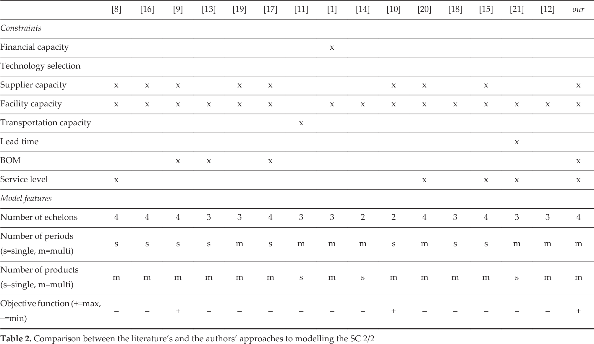
Papageorgiou (2008) [18], the authors study production-distribution SCs and propose static models. The same problem, but in a dynamic environment, is considered by Yang et al. (2002) [19], Melo et al. (2005) [1], Thahn et al. (2008) [20], and Altiparmak et al. (2009) [21]. In order to evaluate the exhaustiveness of these papers, we propose a classification following four criteria: the strategic decisions evaluated by the models, the economic parameters taken into account, the constraints used, and the models' features. Table 1 summarizes the classification and compares our approach to the literature.

Table 1.

Comparison between the literature's and the authors' approaches to modelling the SC 1/2

	[8]	[16]	[9]	[13]	[19]	[17]	[11]	[1]	[14]	[10]	[20]	[18]	[15]	[21]	[12]	our
Strategic decision
Capacity size				x				x	x		x	x	x	x	x	x
Technology selection				x									x
Sourcing	x	x	x			x		x			x		x	x		x
Facility location	x	x	x	x	x	x	x	x	x	x	x	x	x	x	x	x
Economic parameters
Fixed costs	x	x	x	x		x	x	x		x	x	x	x	x
Variable costs			x	x				x	x	x	x			x
Capital costs											x					x
Production Costs	x	x			x	x		x	x	x	x	x	x	x	x	x
Material costs	x		x			x				x	x		x			x
Labour costs																x
Energy costs																x
Transportation costs	x	x	x	x	x	x	x	x	x		x	x	x	x	x	x
Inventory costs	x		x		x		x	x	x		x	x		x	x	x
Pipeline inventory costs							x
Exchange rate															x	x
Taxes			x												x
Prices			f							f
Demand (v=variable, f=fixed)	f	f	f	f	v	f	v	v	v	f	v	f	f	v	v	v

From the summary in Table 1, it is evident that the aim of this work is to fill an existing gap in the literature, through the proposal of a calculation model that includes all the economic parameters while also considering a variable demand rate.

Moreover, this model also deals with the general capacity of supply chains to avoid the main risks that are presented to them, underlined many times by many authors as one of the most important issues of supply chain management. The identification, assessment and management of risks represents an important issue in all fields of management engineering, on which many contributions have been produced over the last few years. Many applications of risk management and assessment have been attempted in the field of project management [22,23], in operations management [24,25,26], in the field of safety in operations management [27,28], and in system size decisions [29]. Therefore, this model could also be used as a departure point for the identification, assessment and management of risks in the supply chain, starting from the fact that generally such risks are not often evaluated using quantitative methods, while this model has a substantial quantitative approach.

3. Model description

In order to address the problem of strategic planning and supply network design, with the hypothesis of decentralized purchasing delocalization, we propose a model built on an objective function based on profit maximization.

Table 2.

Comparison between the literature's and the authors' approaches to modelling the SC 2/2

	[8]	[16]	[9]	[13]	[19]	[17]	[11]	[1]	[14]	[10]	[20]	[18]	[15]	[21]	[12]	our
Constraints
Financial capacity								x
Technology selection
Supplier capacity	x	x	x		x	x				x	x		x			x
Facility capacity	x	x	x	x	x	x		x	x	x	x	x	x	x	x	x
Transportation capacity							x
Lead time														x
BOM			x	x		x										x
Service level	x										x		x	x		x
Model features
Number of echelons	4	4	4	3	3	4	3	3	2	2	4	3	4	3	3	4
Number of periods (s=single, m=multi)	s	s	s	s	m	s	m	m	m	s	m	s	s	m	m	m
Number of products (s=single, m=multi)	m	m	m	m	m	m	s	m	s	m	m	m	m	s	m	m
Objective function (+=max, -=min)	−	−	+	−	−	−	−	−	−	+	−	−	−	−	−	+

3.1 Hypotheses

In this model, we have adopted the activity-based methodology proposed by Vila et al. (2006) [14]. An activity can be defined as a set of resources that, using a certain technology, transforms one or more inputs into one or more outputs. Additionally, materials warehousing must be considered an activity. Moreover, a bi-injective relationship between a technology and an activity is imposed. In other words, every activity uses just one technology and vice versa. Furthermore, a number of hypotheses are assumed in the model implementation. In order to make the model dynamic, demand and production costs are considered variable over the planning horizon; in order to make the SC design as realistic as possible, it is considered multiechelon, multi-country, multi-facility, and multi-product; and to reduce duplication of activities, we assume that activity capacity cannot be split in a relocation process. In other words, an activity can be performed only in a single facility.

3.2 Strategic decision

In order to integrate the main strategic decisions concerning SC design and planning, we introduced several decision variables into the model that relate to facility-location, capacity-sizing and sourcing strategies. Facility-location decisions usually concern the problem of where to locate facilities throughout the SC. In our model, the aim is to identify the optimal SC structure: that is, to determine how many and which facilities should be opened and/or closed; where each facility should be located in a predefined set of potential sites (already existing or not); and in which facility each activity should be allocated. In the literature, capacity-sizing decisions are typically addressed through a scenario analysis, with the aim of identifying the most robust values for global output. Since the identification of the global capacity of the SC lies outside of the model's objectives, we focused our attention on the possibility of increasing the capacity for each activity. Therefore, global capacity is predefined, whereas each activity can exploit extra capacity up to a certain cost. Sourcing decisions are normally connected with choosing suppliers, in terms of cost, quality, and reliability, and choosing the optimal number of suppliers and purchased items per supplier. In our model, we have considered a set of potential suppliers (existing or not), each with a certain level of capacity, from which the model chooses the best in terms of costs. Moreover, the quantity of raw materials provided by each supplier is identified. According to Shehabuddeen et al. (2006) [30], in making decisions about technology selection, a company needs to consider a wider set of parameters beyond financial aspects. In particular, internal factors (such as quality, reliability, flexibility, volume, etc.), external factors (such as customer needs, supplier technology, environmental laws, etc.), and financial factors can affect the choice of one technology over another. For this reason, we have not included technology-selection decisions in the model.

3.3 Modelling blocks

The objective function maximizes the total profits of the SC at the end of the planning horizon. In order to make a model dynamic, several parameters are considered variable, as the function of a discrete time period that is in turn divided into a certain number of periods. This function can be divided into four macro-blocks relating to specific cost drivers: investments, labour and energy, sourcing, and logistics. Moreover, a further block can be considered for revenues. The parameters chosen for each group are described in the following paragraphs.

3.3.1 Investments

In the scenario considered by this paper, investment costs are highly influenced by the transferring of activities between facilities. Typically, a firm uses two main approaches to relocate activities: first, relocating the activity by transporting its resources from the origin site to the destination site; and second, relocating the activity by dismantling resources from the origin site, and acquiring and installing new resources in the destination site. In order to make the model as general as possible, our methodology neglects this difference, considering only the total cost that a firm must incur in case of activity relocation. However, two drivers that can have significant effects on the cost of SC reconfiguring are the costs of opening and the costs of closing a facility. The former pertains to cases in which a firm delocalizes an activity when it does not yet have a new facility, whereas the latter pertains to cases in which a firm relocates all the activities from a particular facility. Moreover, the closing costs can be assumed positively or negatively as a function of both the resource typology (human or physical) and the relocation approach. Finally, although some authors suggest not retaining costs for the capital depreciation variable as a function of the countries (Beckman and Rosenfield, 2006) [2], we have nevertheless accounted for them, since the depreciation rules in developing countries can change rapidly or can be different from the rules of the origin country.

3.3.2 Labour and energy

From the literature review, it is noticeable that many researchers aggregate operations costs without handling labour and energy costs separately. However Hammami et al. (2008) [3] and Paulonis and Norton (2008) [7] suggest evaluating the effects of these parameters by isolating their drivers. Therefore, we have considered both labour and energy costs in the model. In particular, labour costs have been split into two factors. Indeed, when a firm delocalizes activities to developing countries, it must consider a tradeoff between the savings derived from lower wages and the expenses involved in labour training. In fact, in order to exploit technological and cultural gaps between developed and developing countries, firms should invest a significant quantity of money in education. On the other hand, energy costs can be modelled with a single driver that changes as a function of activity capacity. Thus, in our approach, energy is considered a fixed cost, which is generally the case in most industries.

3.3.3 Sourcing

One purpose of delocalization is to access the low-cost raw materials and components that developing countries offer. Although these kinds of choices can improve the economical performances of a firm, some trade-off aspects must be considered. In particular, the usage of delocalized suppliers can affect the firm's efficiency in terms of customer satisfaction. Indeed, the quality and availability of the delocalized suppliers may be much worse than the original ones. For this reason, whenever a developing country vendor is chosen, a firm should implement action plans to train the suppliers on quality and availability issues, and to integrate their own production network with that of the supplier, in terms of both physical and informative flows. Therefore, in our model, we have considered a cost driver for raw materials, which is variable as both the function of the supplier and a fixed cost for the supplier's education/integration.

3.3.4 Logistics

Typically, SC models take into account both transportation and inventory costs. In our model, we have considered only the former. In fact, the stocking process can be considered a non-value-added activity, and, consequently, it can be addressed like any other activity. Moreover, transportation costs represent an important balance factor in configuring an SC, especially in delocalization hypotheses. In particular, these costs are usually in trade-off with savings derived from activity relocation. Indeed, according to Hammami et al. (2008) [3], there have been several cases in which companies have delocalized production activities without evaluating the effects on transportation costs, resulting consequently in less profitable conditions. Typically, transportation costs include the costs for transporting a product from the origin to the destination, and the costs of risks connected with transportation and duties in the case of international deliveries. In order to reduce the number of computations elaborated by the model, we have aggregated all of these aspects into a single driver. Indeed, it is not difficult for a company to evaluate the global costs connected with transportation. Conversely, we have introduced a differentiation between the highest and lowest echelons of a given mode of transportation. In fact, using overseas (or foreign) suppliers, delocalizing production activities (or relocating distribution centres) can significantly affect logistics costs. Thus, in order to isolate the single effect of these actions, we considered three possible types of transportation: supplier-to-plant, plant-to-plant, and plant-to-distribution-centre.

3.4 Mathematical formulation

The following notation is used to define the mathematical model:

SETS AND INDICES

PH	planning horizon (years);
T	number of periods in the planning horizon;
A	set of production/logistical activities;
S	set of potential production/logistical facilities;
R	set of raw materials;
P	set of products;
FP	set of finished products;
P(a)ⁱⁿ	set of input products of activity a, P(a)ⁱⁿ⊂P;
P(a)ⁱⁿ	set of output products of activity a, P(a)ⁱⁿ⊂P;
R(a)	set of raw materials (or components) of activity a, R(a)⊂RM;
FP(a)	set of finished products of activity a, FP(a)⊂FP;
DC	set of distribution centres;
V	set of suppliers (used or not);
t	period, tεT;
i	site, iεS;
a	activity, a εA;
v	supplier, vεV;
p	product, pεP;
f	finished product, f ε PF;
r	raw material, rεRM;
d	distribution centre, dεDC.

DECISION VARIABLES

Binary variables

x_ia	0 if activity a is not located at facility i, 1 if activity a is located at facility i;
α_i	0 if facility i is not open, 1 if facility i is open;
β_i	0 if facility i is not closed, 1 if facility i is closed;
γ_{i→i’, a}	0 if activity a is not transferred from facility i to facility i‘, 1 if activity a is transferred from facility i to facility i’;
δ_a ^(t)	0 if $\sum_{p = 1}^{P} y_{p}^{(t)} - K_{a} \leq 0$ during period t; 1 otherwise;
s	0 if supplier s is not used, 1 if supplier s is used.

Integer variables

q_f ^(t)	quantity of finished products f to deliver at period t;
w_vr ^(t)	quantity of raw materials (or components) r purchased from supplier v at period t;
y_p ^(t)	quantity of products p to produce at period t;
z ^(t) _v→i,r	quantity of raw materials (or components) r delivered from supplier v to facility i at period t;
z ^(t) _i→i,p	quantity of products p to transfer from facility i to facility i' at period t;
z ^(t) _i→d,f	quantity of products p to transfer from facility i to distribution centre d at period t.

PARAMETERS

D_f ^(t)	demand of finished products f for period t;
e_i ^(t)	exchange rate of facility i at period t;
e_v ^(t)	exchange rate of supplier s at period t;
AV_a	technology value of activity a per capacity unit;
K_a	preassigned output capacity of activity a;
DER_i	annual depreciation rate for facility i at period t;
Dim_a	necessary space for activity a per capacity unit;
FO_i	cost per space unit of facility i;
FC_i	closing cost for facility i;
KT _i→i _{, a}	necessary cost to transfer activity a from facility i to facility i';
KA_ia	cost of capacity acquisition, per quantity unit, for activity a in facility i;
BOM_fp	BOM coefficient of product p for finished product f;
AL L_ap	0 if product p is not worked on by activity a, 1 if product p is worked on by activity a;
L T_ia ^(t)	cost, per capacity unit, of labour training & education for activity a in facility i at period t;
L_ia ^(t)	cost, per capacity unit, of labour for activity a in facility i at period t;
E_ia ^(t)	cost, per capacity unit, of energy for activity a in facility i at period t;
BOMR_fr	BOM coefficient of raw material r for finished product f;
RM_vr ^(t)	unit cost of raw material (or component) r for supplier v at period t;
VK_vr ^(t)	capacity of material r for supplier v at period t;
TRR_v→i,r ^(t)	unit cost to transfer raw material (or component) r from supplier v to facility i, at period t;
SM_v ^(t)	fixed management cost (integration, ICT, training and education, etc.) for supplier v at period t;
TRP ^(t) _{i →d,p}	unit cost to transfer product p from facility i to facility i' at period t;
TRP ^(t) _{i →i,p}	unit cost to transfer product p from facility i to distribution centre d at period t;
AL L_af	0 if finished product f is not worked on by activity a, 1 if finished product f is worked on by activity a;
PR_f ^(t)	unit price of finished product f at period t.

OBJECTIVE FUNCTION COMPONENTS

Activity depreciation costs

\sum_{t = 1}^{T} \sum_{i = 1}^{S} \sum_{a = 1}^{A} e_{i}^{(t)} \cdot A V_{a} \cdot K_{a} \cdot \frac{P H \cdot D E R_{i}}{T} \cdot x_{i a}

(1)

Facility opening costs

\sum_{t = 1}^{T} \sum_{i = 1}^{S} \sum_{a = 1}^{A} e_{i}^{(t)} \cdot D i m_{a} \cdot K_{a} \cdot F O_{i} \cdot \frac{P H \cdot D E R_{i}}{T} \cdot α_{i}

(2)

Facility closing costs

\sum_{i = 1}^{S} e_{i}^{(t)} \cdot F C_{i} \cdot β_{i}

(3)

Costs for a transfer of activities

\sum_{t = 1}^{T} \sum_{a = 1}^{A} e_{i}^{(t)} \cdot K T_{i \to i', a} \cdot \frac{P H \cdot D E R_{i'}}{T}

(4)

Costs for a transfer of a single activity

\sum_{t = 1}^{T} \sum_{i = 1}^{S} \sum_{a = 1}^{A} e_{i}^{(t)} \cdot K A_{i a} \cdot (\sum_{p = 1}^{P {(a)}^{o u t}} y_{p}^{(t)} - K_{a}) \cdot δ_{a}^{(t)} \cdot x_{i a}

(5)

where $y_{p}^{(t)} = \sum_{f = 1}^{F P} B O M_{f p} \cdot q_{f}^{(t)}$

Labour costs

\sum_{t = 1}^{T} \sum_{i = 1}^{S} \sum_{a = 1}^{A} e_{i}^{(t)} \cdot (L T_{i a}^{(t)} + L_{i a}^{(t)}) \cdot K_{a} \cdot x_{i a}

(6)

Energy costs

\sum_{t = 1}^{T} \sum_{i = 1}^{S} \sum_{a = 1}^{A} e_{i}^{(t)} \cdot E_{i a}^{(t)} \cdot K_{a} \cdot x_{i a}

(7)

Material costs

\sum_{t = 1}^{T} \sum_{i = 1}^{S} \sum_{a = 1}^{A} \sum_{r = 1}^{R (a)} e_{i}^{(t)} \cdot R M_{υ r}^{(t)} \cdot w_{υ r}^{t ()}

(8)

Supplier management costs (training and integration)

\sum_{t = 1}^{T} \sum_{v = 1}^{V} e_{i}^{(t)} \cdot S M_{υ}^{(t)} \cdot ϵ_{υ}

(9)

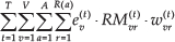
Transportation costs – supplier-to-plant

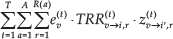
\sum_{i = 1}^{T} \sum_{a = 1}^{A} \sum_{r = 1}^{R (a)} e_{υ}^{(t)} \cdot T R R_{υ \to i, r}^{(t)} \cdot z_{υ \to i' r}^{(t)}

(10)

Transportation costs – plant-to-plant

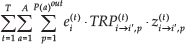
\sum_{i = 1}^{T} \sum_{a = 1}^{A} \sum_{p = 1}^{P {(a)}^{o u t}} e_{i}^{(t)} \cdot T R P_{i \to i', p}^{(t)} \cdot z_{i \to i' p}^{(t)}

(11)

Transportation costs – plant-to-DC

\sum_{i = 1}^{T} \sum_{a = 1}^{A} \sum_{f = 1}^{F P (a)} e_{i}^{(t)} \cdot T R F_{i \to d, p}^{(t)} \cdot z_{i \to d, f}^{(t)}

(12)

Revenues

\sum_{t = 1}^{T} \sum_{f}^{F P} P R_{f}^{(t)} \cdot q_{f}^{(t)}

(13)

The problem can be formulated as follows:

\begin{array}{l} M a x (Z) = & (13) - (1) - (2) - (3) - (4) - (5) - (6) + \\ - (7) - (8) - (9) - (10) - (11) - (12) \end{array}

(14)

It is subjected to the following constraints:

\sum_{i = 1}^{S} x_{i a} = 1, \forall a \in A

(15)

w_{υ r}^{(t)} \sum_{i = 1}^{S} z_{υ \to i, r'}^{(t)} \forall υ \in V, \forall r \in R, \forall t \in T

(16)

\begin{array}{l} A L L_{a p} \cdot y_{p}^{(t)} \cdot x_{i a} = \sum_{i' = 1}^{S} z_{i \to i', p'}^{(t)} \\ \forall i \in S, \forall a \in A, \forall p \in P, \forall t \in T \end{array}

(17)

\begin{array}{l} A L L_{a f} \cdot q_{f}^{(t)} \cdot x_{i a} = \sum_{d = 1}^{D G} z_{i \to d, f'}^{(t)} \\ \forall i \in S, \forall a \in A, \forall f \in F P, \forall t \in T \end{array}

(18)

w_{υ r}^{(t)} \leq V K_{υ r}^{(t)}, \forall υ \in V, \forall r \in R, \forall t \in T

(19)

\sum_{υ = 1}^{V} w_{υ r}^{(t)} = \sum_{f = 1}^{F P} B O M R_{f r} \cdot q_{f}^{(t)}, \forall r \in R, \forall t \in T

(20)

q_{f}^{(t)} \leq D_{f}^{(t)}, \forall f \in F P, \forall t \in T

(21)

The objective function maximizes the total profits of the SC. Constraint (15) represents the necessity of locating an activity in a single facility, according to the model hypotheses. Constraints (16), (17), and (18) enforce flow conservation. In particular, they respectively impose the following: that the quantity of raw materials transported from a supplier to a facility is equal to the quantity sourced from that supplier; that the quantity of products transported from a facility to another is equal to the quantity produced by the starting facility; and that the quantity of finished products transported from a facility to a DC is equal to the quantity produced by the facility itself. Constraint (19) represents the supplier capacity; it imposes that the quantity of raw materials sourced from each supplier is less than or equal to the capacity of the supplier. Constraint (20) imposes that the purchased quantity of raw materials is equal to the required quantity for producing the volume of finished products, as defined by the model. Constraint (21) imposes that the quantity of products to produce is less than or equal to the quantity requested by the market (or demand). Moreover, the variable d_a ⁽ ^t) allows for the expansion of an activity's capacity, but only by incurring a further cost for the capacity acquisition.

4. Experimental results

Due to the problem's complexity, an exact solution to the objective function could not be found for real SCs. Therefore, we have addressed model optimization through the genetic algorithm toolbox for use with the commercial software MATLAB R2011b. All experiments were conducted on an Intel Xeon, equipped with four processors of 2.4 GHz and 8GB RAM. In order to assess the model quality in terms of applicability and flexibility, we developed a methodology constituted by three kinds of analysis:

Performance analysis, aiming to test the model in terms of calculation time. In particular, the single and global effects of the model parameters were evaluated, in order to understand which of them were most influential on calculation time. Moreover, this analysis provided indications on SC features for the successive scenario analysis.

Convergence analysis, which addressed the problem of a stopping criterion for the genetic algorithm. In particular, a group comprising four SC structures with different complexities was tested, in order to identify the number of cycles after which the algorithm provides solutions with a good trade-off between calculation time and quality of the solution.

Scenario analysis, to evaluate the model's applicability and flexibility with respect to realistic business conditions. In particular, 12 scenarios, representative of different industries, were solved through the model, thus proving its quality.

4.1 Performance analysis

Performance analysis is targeted to define the correlation between the SC's complexity and the calculation time of the objective function. To identify this relationship, we firstly considered sets on which the model is dependent: number of periods, number of facilities, number of activities, number of finished products, number of semi-finished products, number of raw materials, and number of suppliers. Secondly, we identified five realistic dimensions for each set. Then, in order to evaluate the single effect of each set, we designed five SC structures per set by changing the dimensions of the set in the analysis and maintaining the same dimensions of the others. Thus, we obtained a group of 29 SC structures in total. Moreover, in order to evaluate the global effect of the model sets, we designed a further four SC structures, starting from the smallest dimensions for each set and increasing them simultaneously. Successively, model parameters were randomly generated from a normal distribution. Although this last procedure does not identify realistic scenarios, it was valid for performance analysis purposes. In fact, calculation time depends only on the SC structure and not on the signs or values of the model parameters. Finally, each of the 33 designed scenarios was run 10 times, measuring the calculation time of the objective function. Figures 1 –8 summarize the results obtained from the performance analysis.

Figure 1.

Effect of periods on calculation time

Figure 2.

Effect of facilities on calculation time

Figure 3.

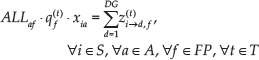
Effect of activities on calculation time

Figure 4.

Effect of finished products on calculation time

Figure 5.

Effect of semi-finished products on calculation time

Figure 6.

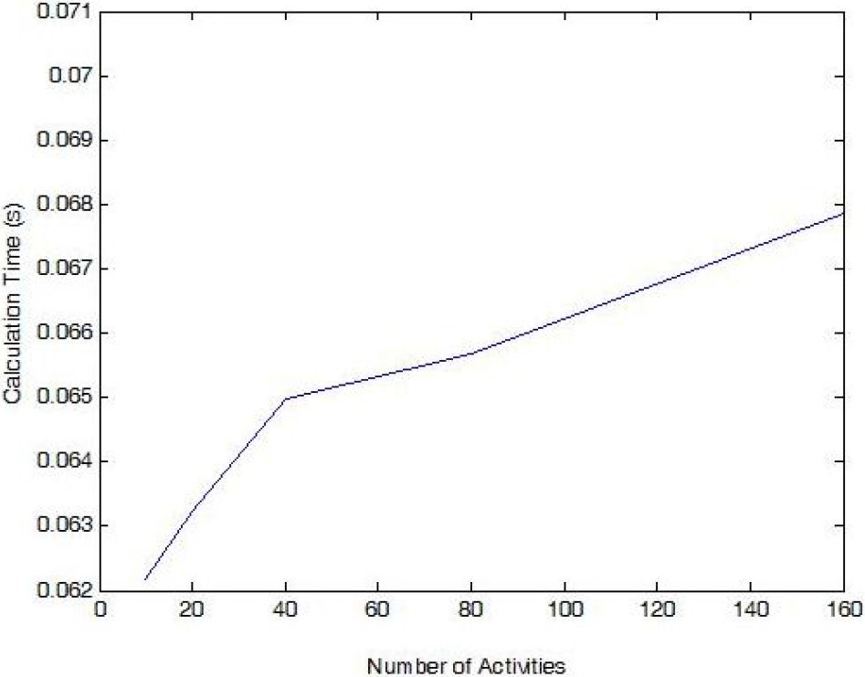
Effect of raw materials on calculation time

Figure 7.

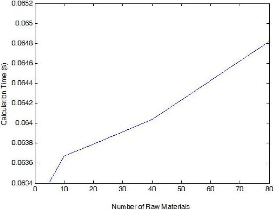
Effect of suppliers on calculation time

Figure 8.

Global Effect on calculation time

In terms of their effect on calculation time trends, the parameters can be clustered into four groups: (i) sets with a linear trend, such as periods and facilities; (ii) sets with a linear trend after a decreasing slope, such as activities and finished products; (iii) sets with a linear trend after an increasing slope, such as raw materials and suppliers; and (iv) a set with an exponential trend, in the case of semifinished products. This final exception is an easy-to-understand phenomenon, since such a parameter will have a strong effect on the complexity of SC transportation and the related number of calculations. Continuing the analysis of the effects of the model sets, we should emphasize that the two parameters with a statistically significant effect on calculation time are the number of periods and the number of semi-finished products, whose average percentage increases are, respectively, 1.39% and 1.32%. Moreover, we can report the average required time per number of periods and per number of semi-finished products, which is, respectively, 2.55·10⁻² s and 2.73·10⁻³ s. Conversely, the sets that least affect calculation time are the number of activities and the number of raw materials, with respective average percentage increases of 0.06% and 0.03%, and respective average required time per unit of 2.45·10⁻³ s and 4.93·10⁻³ s. Finally, some considerations can be made regarding the global effect of the model sets. In particular, calculation time displays a linear trend, with a average percentage increase of 0.22% and a required time per number of variables of 2.38·10⁻⁴ s. Although these values are congruent with those concerning a single set, there is a change of magnitude. In fact, due to the multiplicative effect of set combination, the calculation time of the objective function grows from tenths of seconds to tens of a second. This aspect suggests that optimizing an SC with a high degree of complexity would consume a relatively high quantity of time. In spite of this, the time results are reasonable if compared with the typical planning horizon for this kind of problem (five or more years).

4.2 Convergence analysis

Once the relationship between the SC complexity and the calculation time of the objective function is understood, the next step is to perform a convergence analysis with the aim of identifying the minimum number of cycles required to obtain a good solution through the MATLAB algorithm. We defined the required number of cycles necessary to achieve algorithm convergence, obtained when the dynamic average of the solutions does not change by more than 0.1% for a successive 50 cycles. In order to perform the convergence analysis, part of the previous data has been recycled. Specifically, the first four scenarios relating to the global effect analysis have been used (Table 3).

To obtain statistically significant results, each scenario was run 10 times, which allowed the dynamic average to be evaluated after each run. Figure 9 shows the mean values of the dynamic average for each scenario (average value of solution/initial solution), against the number of cycles¹. Moreover, a vertical line that crosses the dynamic average function has been added to represent the number of necessary cycles for convergence.

Figure 9.

Dynamic average vs. number of cycles for scenarios of convergence analysis

Table 3.

Features of the scenarios used for convergence analysis

# of	periods	facilities	activities	raw materials	semi-finished products	finished products	suppliers	variables
Scenario 1	1	2	10	5	10	2	10	82
Scenario 2	2	4	20	10	20	4	20	528
Scenario 3	4	8	40	20	40	8	40	3 712
Scenario 4	8	16	80	40	80	16	80	27 648

By analysing this figure, it can be noted that the number of necessary cycles required to reach convergence using MATLAB R2011b's genetic algorithm toolbox is relatively small. In fact, it is fewer than 120 cycles for Scenario 4, which represents a complex SC. This outcome suggests that planning and/or designing SCs using the combination of our model and the MATLAB optimization tool requires a relatively short time. Indeed, only five hours were necessary to run Scenario 4, 10 times, with a stopping criterion of 150 cycles (approximately 1.5 times the required number of cycles). Finally, we studied the relationship between the number of necessary cycles and the number of model variables (Figure 10). Hence, it is possible to see that the trend of convergence as a function of the model variables is asymptotic with a decreasing slope. This result suggests that SC features affect the total calculation time for more than the algorithm convergence. This is particularly true for those SCs whose complexity is higher than that used in this analysis.

Figure 10.

Required number of cycles for convergence vs. number of model variables

4.3 Scenario analysis

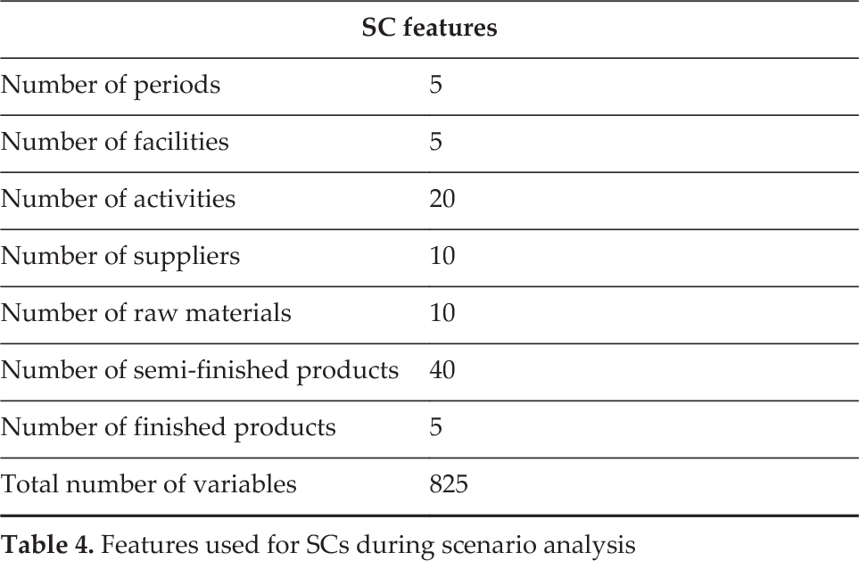
Starting from the performance and convergence analyses, we implemented an experiment campaign aimed to verify the model's flexibility and applicability in real contexts. This campaign was based on the application of our model to 12 realistic scenarios, representing several industries. In the first step, the SC features, in terms of complexity, were chosen. In particular, using the results of sensitive analysis, we defined the dimensions of the model sets to obtain a good trade-off between the concreteness of the SC and the solving time of the model. Table 4 shows the features of the SCs used during the scenario analysis.

Table 4.

Features used for SCs during scenario analysis

	SC features
Number of periods	5
Number of facilities	5
Number of activities	20
Number of suppliers	10
Number of raw materials	10
Number of semi-finished products	40
Number of finished products	5
Total number of variables	825

Following this, 12 scenarios were identified to cover several industries. In order to generate realistic data, two aspects that highly affect market features were considered: product BOM shapes and product cost structures. Specifically, we assumed that BOM shapes can be cylindrical, convergent, divergent and convergent-divergent, and that cost structures can be capital-intensive, labour-intensive and balanced. By crossing each kind of BOM shape with each kind of cost structure, most industries are represented (i.e., a cylindrical BOM shape with a capital-intensive cost structure is characteristic of the chemicals market, whereas a convergent-divergent BOM shape with a balanced cost structure is typical of the automotive sector, etc.). The parameters used for each scenario are reported in Table 5.

Table 5.

Features used for supply chains during scenario analysis

	BOM shape	Cost structure
Scenario 1	Cylindrical	Balanced
Scenario 2	Cylindrical	Labour-intensive
Scenario 3	Cylindrical	Capital-intensive
Scenario 4	Convergent	Balanced
Scenario 5	Convergent	Labour-intensive
Scenario 6	Convergent	Capital-intensive
Scenario 7	Divergent	Balanced
Scenario 8	Divergent	Labour-intensive
Scenario 9	Divergent	Capital-intensive
Scenario 10	Convergent-divergent	Balanced
Scenario 11	Convergent-divergent	Labour-intensive
Scenario 12	Convergent-divergent	Capital-intensive

In this case, the generation of model parameters has been constrained by the SC features, product BOM shapes and product cost structures, in order to obtain the model parameters as a function of the cost-driver weight, the country in which an activity is performed, and material flows. Although the number of required cycles for the selected SCs is around 50, we preferred to set it to 150 in order to achieve a more robust approach. Each scenario was run 30 times, and the results tracked in terms of solution quality and calculation time. Table 6 summarizes the results obtained by the scenario analysis. The “Initial value” column represents profit in the starting configuration of the SC, where all facilities and all suppliers are located in a developed country and production quantity corresponds to market demand. The “μ” column represents the average of 30 repetitions of outputs, provided by MATLAB R2011b's genetic algorithm tool. The “σ” column is the standard deviation of solutions obtained from 30 repetitions. The “μ Increase” column represents the percentage ratio between the average value and the initial value. The “μ Time” and “σ Time” columns are, respectively, the average and standard deviation of solving time for 30 repetitions.

Table 6.

Output of analysis for each scenario

	Initial value	μ	σ	μ Increase	μ Time	σ Time
	(€)	(€)	(€)	%	(s)	(s)
Scenario 1	−2.66E+09	−1.26E+10	5.86E+08	475%	58.2	0.82
Scenario 2	−7.25E+09	−1.87E+10	5.88E+08	258%	57.7	0.22
Scenario 3	−5.17E+09	−1.30E+10	1.05E+09	251%	57.8	0.17
Scenario 4	−2.85E+09	−1.22E+10	4.72E+08	429%	58.5	2.03
Scenario 5	−1.20E+10	−2.11E+10	1.36E+09	176%	65.8	0.19
Scenario 6	−6.23E+09	−1.27E+10	8.46E+08	205%	65.5	0.30
Scenario 7	−5.92E+09	−1.47E+10	3.52E+08	247%	65.2	0.16
Scenario 8	−9.82E+09	−1.92E+10	1.14E+09	195%	65.2	0.20
Scenario 9	−6.40E+09	−1.38E+10	4.02E+08	215%	65.2	0.19
Scenario 10	−5.28E+09	−1.42E+10	5.34E+08	270%	65.6	0.19
Scenario 11	−1.00E+10	−1.94E+10	1.69E+09	194%	65.0	0.29
Scenario 12	−7.22E+09	−1.28E+10	7.63E+08	178%	65.1	0.16

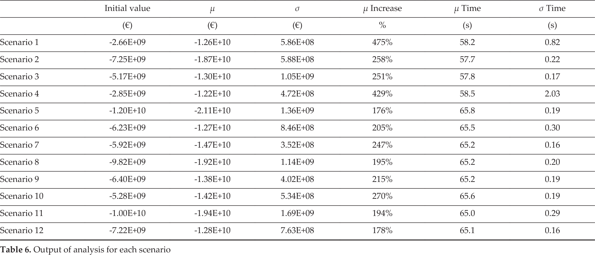
By analysing the table, it can be noted that the model displays an average increase in function value of 258%, with a minimum of 176% and a maximum of 475%. This result indicates that a firm in the same initial conditions as one of these scenarios could incrementally increase its profits considerably. Although this cannot be demonstrated using a real case, the results of this scenario analysis in terms of solution quality prove that the model is applicable in real industries and flexible enough to be applied to the majority of markets. At the same time, the average calculation time was 63 seconds, with a lowest value of 58 seconds and a highest of 66 seconds. This outcome is congruent with the results of the sensitivity and convergence analyses. Thus, the model quality has also been proved in terms of the time required to plan and design SCs.

By aggregating data as a function of BOM shapes and cost structures, further outputs can be produced (6). In particular, according to Figure 11, the optimization performances of the cylindrical BOM (Scenarios 1, 2, and 3) were higher compared to those of other shapes. Indeed the average increase in solution for this shape was 328%, as opposed to 270% for the convergent shape, 219% for the divergent shape, and 214% for the convergent-divergent shape. On the other hand, the performances of the balanced cost structure (Scenarios 1, 4, 7, and 10) were higher than those of the others, with an average increase of 355%, against 212% for the capital-intensive structure and 206% for the labour-intensive structure.

Figure 11.

Average increase of the solution as a function of BOM shapes and cost structures

Table 7.

Configuration of BOM shapes and cost structures

Configuration	Scenario
Cylindrical	1, 2, 3
Convergent	4, 5, 6
Divergent	7, 8, 9
Convergent-divergent	10, 11, 12
Balanced	1, 4, 7, 10
Labour-intensive	2, 5, 8, 11
Capital-intensive	3, 6, 9, 12

Finally, Figure 12 shows that the cylindrical shape presents a much lower solving time with an average of 58 seconds, whereas, in all the other cases, the equivalent value is always equal to or greater than 62 seconds.

Figure 12.

Average calculation time as a function of BOM shapes and cost structures

5. Conclusions

In this paper, a mathematical model for the strategic planning and design of SCs in global contexts is proposed. The model is dynamic and suited to delocalization problems. It permits researchers to identify the optimal SC configurations in terms of facility location, market fulfilment, and supplier selection (with the relative quantity of raw materials to buy for each of them). Our approach has several novelties when compared to the literature:

it extends the existing models by introducing a better cost segmentation, with particular attention given to labour and energy drivers;

it considers multi-echelon, multi-period and multi-product SCs; and

it integrates capacity-sizing, sourcing and facility-location decisions.

The proposed model was solved using the genetic algorithm toolbox for use with the commercial software MATLAB R2011a, with reasonable computational times. A group of 12 scenarios were tested, proving the flexibility and applicability of the model in different industrial cases. Although experimental results are good, further improvements could still be implemented; this might include information about product quality, backlog effects, and the risks connected with activity delocalization. Finally, we suggest that another extension of the work could be the integration of market-access considerations, in order to make the model even more general.

Footnotes

1

MATLAB GA manages only minimization problems, and thus the objective function had to be inverted.

References

Melo

M.T.

Nickel

, and da Gama

Saldanha F.

Dynamic multi-commodity capacitated facility location: A mathematical modeling framework for strategic supply chain planning. Computers & Operations Research, 33:181–208, 2005.

Beckman

S.L.

and Rosenfield

D.B.

Operations Strategy: Competing in the 21st Century. McGraw-Hill Irwing, 2006.

Hammami

Frein

, and Hadj-Alouane

A.B.

Supply chain design in the delocalization context: Relevant features and new modeling tendencies. Int. J. Production Economics, 113:641–656, 2008.

Manzini

and Bindi

Strategic design and operational management optimization of a multi stage physical distribution system. Transportation Research Part E, 45:915–936, 2009.

Aguilar-Sevén

R. S.

Business process modelling: Review and framework. Int. J. Production Economics, 90:129–149, 2004.

Lambiase

Mastrocinque

Miranda

, and Lambiase

Strategic planning and design of supply chains: A literature review. International Journal of Engineering Business Management, 5:1–11, 2013.

Paulonis

and Norton

McKinsey global survey results: Managing global supply chains. The McKinsey Quarterly, pages 1–9, 2008.

Sabri

E.H.

and Beamon

B.M.

A multi-objective approach to simultaneous strategic and operational planning in supply chain design. Omega, 28:581–598, 2000.

Vidal

C.J.

and Goetschalckx

A global supply chain model with transfer pricing and transportation cost allocation. European Journal of Operational Research, 129:134–158, 2001.

10.

Shen

Max Z.J.

and Qi

Incorporating inventory and routing costs in strategic location models. European Journal of Operational Research, 179:372–389, 2007.

11.

Ambrosino

and Scutellá

M.G.

Distribution network design: New problems and related models. European Journal of Operational Research, 165:610–624, 2004.

12.

Georgiadis

M.C.

Tsiakis

Longinidis

, and Sofioglou

M.K.

Optimal design of supply chain networks under uncertain transient demand variations. Omega, 39:254–272, 2011.

13.

Verter

and Dasci

The plant location and flexible technology acquisition problem. European Journal of Operational Research, 136:366–382, 2002.

14.

Vila

Martel

, and Beauregard

Designing logistics networks in divergent process industries: A methodology and its application to the lumber industry. Int. J. Production Economics, 102:358–378, 2006.

15.

Hammami

Frein

, and Hadj-Alouane

A.B.

A strategic-tactical model for the supply chain design in the delocalization context: Mathematical formulation and a case study. Int. J. Production Economics, 122:351–365, 2009.

16.

Jayaraman

and Pirkul

Planning and coordination of production and distribution facilities for multiple commodities. European Journal of Operational Research, 133:394–408, 2001.

17.

Yan

, and Cheng

T.C.E.

A strategic model for supply chain design with logical constraints: Formulation and solution. Computers & Operations Research, 30:2135–2155, 2003.

18.

Tsiakis

and Papageorgiou

L.G.

Optimal production allocation and distribution supply chain networks. Int. J. Production Economics, 111:468–483, 2008.

19.

Yang

Y.-J.

Yang

S.-Y.

Chang

B.-M.

, and Park

A combined model of network design and production/distribution planning for a supply network. Computers & Industrial Engineering, 43:263–281, 2002.

20.

Thanh

P.N.

Bostel

, and Péton

A dynamic model for facility location in the design of complex supply chains. Int. J. Production Economics, 113:678–693, 2008.

21.

Altiparmak

Gen

Lin

, and Karaoglan

A steady-state genetic algorithm for multi-product supply chain network design. Computers & Industrial Engineering, 56:521–537, 2009.

22.

Nenni

M.E.

and Giustiniano

Increasing integration across the supply chain through an approach to match performance and risk. American Journal of Applied Sciences, 10(9):1009–1017.

23.

Marcelino-Sádaba

Pérez-Ezcurdia

Lazcano

Echeverría A.M.

, and Villanueva

Project risk management methodology for small firms. International Journal of Project Management, 32(2):327–340.

24.

, and Feng

Analysis of wind power generation operation management risk in china. Renewable Energy, 64:266–275.

25.

Fragniére

Gondziob

, and Yang

Operations risk management by optimally planning the qualified workforce capacity. European Journal of Operational Research, 202(2):518–527.

26.

Wanga

Lib

O'brienc

, and Lid

A production planning model to reduce risk and improve operations management. Int. J. Production Economics, 124(2):463–474.

27.

Fera

and Macchiaroli

Proposal of a quali-quantitative assessment model for health and safety in small and medium enterprises. In WIT Press, editor, 3rd International Conference on Safety and Security Engineering, SAFE 2009, volume 108, pages 117–126, 2009.

28.

Fana

Loa

C.K.Y.

Ching

, and Kan

C.W.

Occupational health and safety issues in operations management: A systematic and citation network analysis review. Int. J. Production Economics, (158): 334–344.

29.