Sage Journals: Discover world-class research

Abstract

A new method for the planning and autonomous execution of a single-trajectory, velocity-independent, parallel parking manoeuvre for autonomous vehicles is presented. The procedure commences with the identification and pre-selection of a smooth sigmoidal trajectory known as the Gompertz curve in parametric format. Trajectory parameters are determined in real-time during the path-planning phase using an optimization scheme in order to generate a candidate path. The optimization scheme takes into account the maximum steering angles that can be physically realized and checks the generated candidate trajectory for collisions. Thereafter, the trajectory is reparametrized to arc-length format using the cubic interpolation method and the vehicle orientation at every point of the trajectory is deduced. Following that, values of the steering angle(s) are determined. In the final step, the vehicle uses dead-reckoning to follows the arc-length parametrized path in reverse in order to park itself in a single-manoeuvre. The proposed method is substantiated through both extensive simulations and real sensor data.

Keywords

autonomous vehicles parallel parking

1. Introduction

Autonomous vehicle technology has steadily and progressively evolved so tremendously over the last few decades that they are now almost a commercial reality. What started as experimental research in navigation, sensing and perception using small-sized mobile robots in the yesteryears has now fully matured and shifted into full-scale autonomous vehicles. Today, major car manufactures such as Toyota, Nissan and Volkswagen have announced their intentions to commercialize fully or semi-autonomous vehicles in the coming years.

Some of the autonomous capabilities that an autonomous vehicle would exhibit are, including but not limited to, lanekeeping [1, 2], traversable terrain detection [3, 4], road-sign detection [5, 6] and vehicle localization [7]. The ability to autonomously perform parking manoeuvres is also desirable. Of the various types of parking manoeuvres, one of the more arduous ones is known as parallel parking. This is the manoeuvre in which a vehicle attempts to park by reversing into a parking space that is in between of two vehicles parked co-linearly, exemplified in the visualization of Fig. 1. This is not a new problem but rather a well-studied area that has solicited solutions from both academia as well as the automotive industry. However, most of the current generation self-parking solutions can broadly be categorized into two classifications: mechanical solutions and sensor based reactive approaches. The former involves major mechanical modifications to the vehicle body, or a complete redesign, such that either the rear wheels rotate or the car length is retracted reducing the overall vehicle span thereby making the parking manoeuvre easier e.g the Hiriko Fold Electric Vehicle from MIT. In the latter case, sensors are used to assist the vehicle in slowly backing up into “empty space”. The first approach cannot be readily adapted for any arbitrary vehicle due to the major modifications required. In the second approach, the parking manoeuvre is at times slow as the vehicle may make multiple manoeuvres e.g a two-point turn or back and forth corrective manoeuvres and thus hold up and impede any traffic behind it. Therefore, a single-manoeuvre parallel parking motion is desirable.

Figure 1.

Parallel parking

From observation and experience, it is a known and demonstrable fact that there exists a single trajectory that when precisely followed enables parallel-parking the vehicle in one smooth and continuous motion. Conversely, any oversteering or under-steering while following this trajectory leads to deviations which requires corrective manoeuvres. Were it be possible to identify this trajectory, it would be possible to command the vehicle to parallel park itself in a single, smooth and continuous motion such that the vehicle has largely moved into the parking space. Thereafter, additional and often optional manoeuvres would only be for straightening the vehicle inside the parking space (where it would not impede any traffic). That will result in a faster parallel parking manoeuvre and is the core point of this work.

1.1 Related Works, Motivation and Novel Contribution

There has already been much effort expended to the problem of autonomous parking from various perspectives and a plethora of solutions can be found in literature, ranging from hardware solutions like MIT's Hiriko Fold EV to advanced software solutions using fuzzy logic and fuzzy controllers [8, 9]. Some techniques involve using stereovision to detect parking space detection by 3D reconstruction [10]. Other techniques do not involve spontaneous and unaided detection of free parking space but instead search for parking spaces using overhead aerial images acquired previously on which path planning could be subsequently performed [11]. Model Predictive Control (MPC) has been applied in the works of [12, 13] to realize autonomous perpendicular parking in addition to other forms of controllers [15]. A number of works have dealt specifically with devising path planning algorithms for realizing autonomous parking [16, 17]. Latest results include using probabilistic techniques combined with open and closed loop approaches to realize sliding-parking manoeuvres [14]. Further, while car-makers such as Lexus have demonstrated and offer autonomous parallel-parking features, their implementation methods are unpublished. Thus, while it may be initially be considered a solved problem, the following discernible features between our approach and the mentioned works outline the fact there is always room for improvement:

No overhead maps or other priori information is required. Only instantaneous laser scans are required

Vision is not required, thus lighting conditions do not impair results

User-input is not required

That the generated trajectory is a single-manoeuvre one is guaranteed i.e no corrections or two point turns

Vehicle may move at varying but safe speeds

Trajectory generated for entering the parking space can also be used to exit the parking space.

Kinematic model used considers slip and accounts for likely odometry errors

Path planning task is simplified since a path model is pre-selected and only the parameters are determined

Use of the sigmoidal Gompertz trajectory as the path model

Fewer trajectory parameters are involved and two point manoeuvres are avoided

The sum of all the individual differences above thus form the overall contribution of the proposed approach to current autonomous-parking solutions with the single most important difference being the generation of a single-manoeuvre parking trajectory in the form of a Gompertz curve that avoids two-point turns, if one exists.

2. Vehicle Model

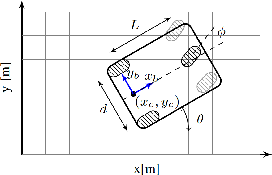
A standard four-wheeled, rear-wheel driven, car-like robot with Ackerman steering is used with the notation assigned to the system as indicated in Fig. 2.

Modelling the car-like robot as a bicycle, the kinematic model is given by

\dot{q} = [\begin{array}{l} {\dot{x}}_{c} \\ {\dot{y}}_{c} \\ \dot{θ} \end{array}] = [\begin{array}{l} v \cos θ \\ v \sin θ \\ v / L \tan ϕ \end{array}]

(1)

where q is the generalized coordinates and v the driving velocity. Neglecting slip, traction and friction etc, this is the most common kinematic model used in literature [19]. However, of the various dynamics that have been unconsidered in this model, slip will be the most prominent source of error in the real world and will need to be considered later.

Figure 2.

Vehicle configuration

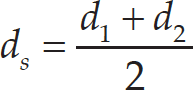
If d₁ and d₂ are the distances travelled by the rear two wheels determined using the encoder ticks, then the midpoint of the rear two wheels (x_c, y_c) travels the distance of

d_{s} = \frac{d_{1} + d_{2}}{2}

(2)

The midpoint of the rear axle (x_c, y_c) is the reference point on the vehicle for the trajectory generation task. Given a trajectory that has been expressed using parametric equations that are parametrized by arc-length, physical data input from d_s can be used to determine the location of this reference point on that trajectory. Together with slip pre-emption, slip-affected positions of the vehicle on the trajectory can be known with sufficient accuracy.

To consider slip in causation of odometry errors, let E denote the 2 × 1 error vector quantifying the dimensions of a two dimensional error ellipsoid signifying slip in the lateral and longitudinal directions of travel as

E = [\begin{array}{l} k_{1} d_{s} \\ k_{2} d_{s} \end{array}]

(3)

with k₁ > k₂ such that E(1) and E(2) are the major and minor axes of an ellipse, respectively, such that

1 = [x y] [\begin{matrix} \frac{1}{E {(1)}^{2}} & 0 \\ 0 & \frac{1}{E {(2)}^{2}} \end{matrix}] [\begin{array}{l} x \\ y \end{array}]

(4)

which describes the error ellipsoid of the aforesaid dimensions centred on the theoretically-correct vehicle position (x_c, y_c). Given that the lateral slip, in the y direction, is practically greater than the longitudinal slip in the x direction, the major axis of the error ellipsoid is taken to be slip in the y direction while the minor axis is slip in x direction. Further, since odometry error increases proportionately to distance travelled, lateral slip E(1) is taken to be a certain percentage of distance travelled, indicated by k₁ and likewise longitudinal slip E(2) is parametrized by k₂.

The vehicle used for real experiments is the RoboCar from ZMP depicted in Fig. 3. A scaled-down version of a fullsized vehicle, this is fully-fledged system with drive train, suspension, and complete steering and camber angle control. There is internal-health monitoring system for operating voltage, power, current and temperature. The robot is equipped with encoders on all wheels, a gyro sensor and a rear-facing laser range scanner. A table of specifications is provided in Table 1.

Figure 3.

RoboCar from ZMP

Table 1.

RoboCar Specifications

Specification	ValueDrive system
Drive system	Drive train, suspension, Ackerman steering
Controller	AMD Geode LX800 Processor 500MHz
Sensors	Stereocamera VGA CCD 30pfs (x2) Single-axis gyro sensor Three-axis acceleration sensor Rotary encoders (x5) Sharp IR GP2Y0A21YK proximity sensors (x8) Hokuyo UTM-30LX laser range scanner
Wireless module	IEEE802.11 b/g/n
Maximum steering	±30°

Figure 4.

Application of Gompertz curve to parallel parking. Trace of reference point on vehicle assumes the shape of a Gompertz curve.

Figure 5.

The Gompertz sigmoid curve and relevant parameters

3 Single Manoeuvre Trajectory Generation

Our proposed approach is to use the sigmoidal Gompertz curve [20] as the model trajectory for realizing a single-manoeuvre, parallel parking motion. The relevance of the sigmoidal Gompertz curve to parallel parking is shown in Fig. 4. One end of the curve is the reference point on the vehicle at initial position and the end point is where the vehicle reference point will come to rest after parallel parking. As is clearly demonstrated, the trajectory of a vehicle performing a parallel parking manoeuvre assumes a sigmoidlike trajectory. This has been verified experimentally. A perfect parallel-parking manoeuvre was executed manually while an external laser range scanner tracked the vehicle movement. The vehicle reference point was acquired from scan data that detected the vehicle edges during the entire manoeuvre. The trace of the vehicle reference point was then seen to be sigmoid-like. Accordingly, the Gompertz curve was subsequently selected from the various sigmoid curves due to the level of manipulation the control parameters offer.

Definition (Gompertz Curve) Let the parameter t be defined on the domain [0, t_end]. Also let $\hat{g} (t) = 〈 x (t), y (t) 〉$ denote a vector-valued, differentiable parametric curve of the form $\hat{g} : ℝ^{n} \to ℝ^{m}$ where x(t) and y(t) are smooth and continuous in an interval. Then, the Gompertz curve of the sigmoid family of curves is expressed in parametric form with t as the parameter, as

\hat{g} (t) = 〈 t, a e^{b e^{c t}} 〉

(5)

for $\forall t \in {0 \leq t \leq t_{e n d}}$ or in non-parametric format as

g (x) = a e^{b e^{c x}}

(6)

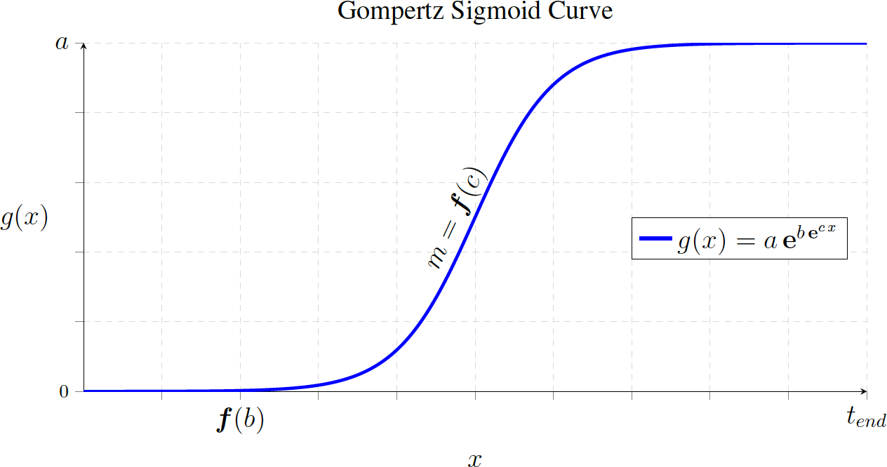
The graph of a Gompertz curve is shown plotted in Fig. 5. The parameters (a, b, c, t_end) form the control points of the Gompertz curve that are available for manipulation to alter the geometrical shape. The most important property, from the perspective of trajectory generation for parallel parking, is that unlike the control points of many other curves, e.g a Bezier curve, each of these parameters influence a single property of the curve. Thus, varying one control point affects only the property to which it is related to and not the overall curve. Henceforth, it is easier to perform path planning by controlling each parameter in succession while other parameters are set static in the context of the parallel parking problem. Thus, instead of generating an entire trajectory during path planning, only the parameters for the Gompertz curve are determined.

3.1 Trajectory Parameter Behaviour and Determination

This section describes how variation of each of the control parameters affects the shape of the Gompertz curve and their role in determining the optimal trajectory for a parallel parking manoeuvre.

Parameter a. Examining equation (6), it is seen that for all t > 1, we have

\lim_{t \to \infty} e^{- c t} = 0

since e^−∞ = 0. It will be pointed out later that c is a non-positive number, thus note the explicit negative sign preceding c. It thus follows that y = ae⁰ and since e⁰ = 1, y = a. Thus, parameter a defines the upper asymptote of the curve and is labelled as such in Fig. 5.

For application in parallel parking, the upper asymptote determines the total width of the Gompertz curve used as trajectory. Thus, the value of a, the curve width, is dependant on the widths of the parking space, the autonomous vehicle, surrounding vehicles and the initial position of the autonomous subject vehicle relative to the parking space. An illustration of how the varying dimensions of the above factors would affect the selection value of a is given in Fig. 6. It is seen that the value of a can be easily varied if the width of the parking space, surrounding vehicles and initial vehicle position vary.

Figure 6.

Example of parameter a variation. Value of a, trajectory width, depends on width of parking space and surrounding vehicles (above) or initial position before commencing parallel parking manoeuvre (below).

Figure 7.

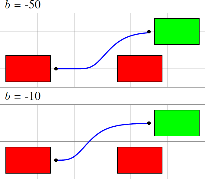
Example of parameter b variation. A value too small implies the vehicle commences alignment to kerb-line too early. While it will may be completely aligned parallel to the kerb-line earlier, there is a risk of collision with the front vehicle (above diagram). Conversely, too high a value implies late commencement of alignment with lesser risk of collision but at the expense of not being aligned parallel to kerb-line after completion of parallel parking (below).

Figure 8.

Example of parameter c variation based on parking space length. A sharper reverse manoeuvre is made in the first case due to constrained space while a smoother turn is made in the second case due to greater parking space being available.

Parameter b. In reference to Fig. 5, parameter b, a nonpositive number, defines the point when the curves starts rising, or in application to parallel parking, when the rear end of the vehicle starts aligning itself parallel to the kerb line. This is first of the parameters to be determined using an optimization scheme devised in later sections. This procedure is reasonable as b may assume a wider range of values compared to parameter a that assumes a single and discrete value that can be instantly determined. Specifically, the value of b determines how soon the vehicle starts aligning parallel to the kerb-line and other vehicles. A higher-than-nominal value implies the vehicle starts aligning itself too late with the possibility the vehicle body will be left at an angle, thereby making it necessary for an additional manoeuvre to align the vehicle robot parallel to the kerb-line. Too small a value means the vehicle rear enters the parking space too soon and is unable to park. This is demonstrated in Fig. 7. Thus, we determine the optimum value through an optimization scheme.

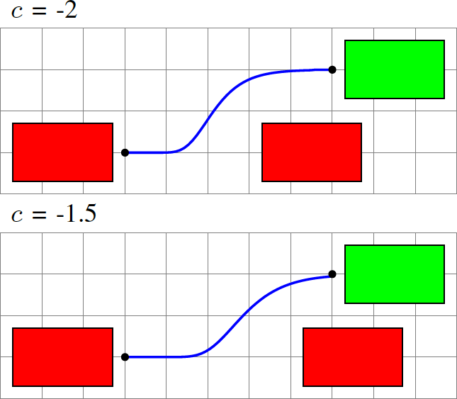
Parameter c. Parameter c, also non-positive, is related but not equal to the slope of the curve. A lower value implies a steeper slope and hence sharper turns whereas a higher value implies a gradual incline and smoother turns. Implication of this property is that the parameter value can be varied depending on the total length of the parking space available. If space is constrained, a lower value can be supplied to this parameter thus realizing a sharper turn into the parking space. Conversely, is space is not constrained, a higher value can be adapted for a smoother entry. This is exemplified in Fig. 8.

Parametert_end. Variable t, which the Gompertz curve is parametrically defined with respect to, is bounded by t_end. Thus, this defines the horizontal length of the curve with one unit of t being equal to one unit length.

3.2 On-line Parameter Determination

It has so far been tacitly assumed that all information necessary for parameter value determination is available e.g length of parking space and width of vehicles parked to the front and rear of the parking space. How can the parallel parking procedure then be utilized for on-line implementation? For on-line implementation, we make use of a laser range scanner. 2D or 3D laser range scanners are a standard sensor on autonomous vehicles to acquire scan data for a 2D or 3D representation of areas. With odometery data and techniques such as SLAM, incremental maps can be constructed although maps are not strictly required in this work. In our procedure, information required for parameter value determination is extracted from instantaneous laser scans acquired from a laser range scanner mounted on the midpoint of the rear vehicle end.

From one such instantaneous laser scan, parameters a; t_end can be instantly determined while values for parameters b and c are resolved by devising iterative optimization schemes. These iterative approaches are necessary since possible values of b, c subsume a range of values and the selected value determines whether or not the generated trajectory is collision-free. This will be treated in later sections.

3.3 Determination of Commanded Steering Angle(s)

Assuming that the correct parallel-parking trajectory and respective parameters have been obtained, the Gompertz curve is then re-parametrized in terms of arc length s. Reparametrization is necessary so that distance travelled d_s can be used to determine the idealized, error-free vehicle position on the arc-parametrized trajectory. Application of the arc length formula

s = \int_{0}^{t_{e n d}} \sqrt{{(\frac{d x}{d t})}^{2} + {(\frac{d_{y}}{d_{t}})}^{2} d t}

(7)

yields the integral expression

s = \int_{0}^{t_{e n d}} \sqrt{1^{2} + (a^{2} b^{2} c^{2} e^{2 b e^{c t} + 2 c t}) d t}

(8)

which can neither be reduced further nor solved analytically. While the value of the total trajectory length (denote this as s_L) can be computed through numerical integration, it is still mandatory to obtain a closed-form solution for eq. (8) such that an expression for arc length s can be obtained as a function of parameter t i.e s(t). Accomplishing that, it is then possible to write an expression for the latter parameter in terms of the former i.e t(s). Substitution of the expression for t(s) into the original parametric equations of eq. (6) parametrized by parameter t will then re-parametrize the equations in with arc length s as the parameter.

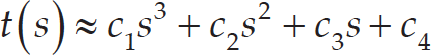
When encountering cases where there are no simple closed form solutions for determining s(t) from which t(s) can be derived, such as the above case, the analytically-irreducible expression can be approximated using the method of cubic interpolation [21]. This involves approximating t(s), which otherwise cannot be obtained through analytical means, using a cubic polynomial. Thus,

t (s) \approx c_{1} s^{3} + c_{2} s^{2} + c_{3} s + c_{4}

(9)

Without delving into the derivations which can be found in [21], the constants of eq. (9) are

c_{1} = \frac{1}{{(s_{L})}^{2}} (c_{3} + \frac{1}{‖ c' (1) ‖}) - \frac{2}{{(s_{L})}^{3}}

(10)

Thus, substitution of eq. (9) using the coefficients founds in eq. (10) into the original t-parametrized parametric equations of eq. (6) leads to the re-parametrized Gompertz curve, as

\hat{g} (s) = 〈 x (s), y (s) 〉

(11)

= 〈 c_{1} s^{3} + c_{2} s^{2} + c_{3} s, a e^{b e^{c (c_{1} s^{3} + c_{2} s^{2} + c_{3} s)}} 〉

(12)

Now let s=s_s be a suitably-chosen sampling distance that represents the distance the vehicle has travelled on the trajectory, as measured by the odometry reading d_s. When increments of this distance i.e {s_s, 2s_s, 3s_s, …, s_L} are substituted into eq. (12), the idealized, error-free vehicle position (x(s), y(s)) at every sampling distance {s_s, 2s_s, 3s_s, …, s_L} is established.

Next, we find find the unit tangent vector at each of the idealized, error-free positions on the trajectory. For a curve g(t | s), whether parametrized by time parameter t or arc length s, the unit tangent vector T(t | s) is given by

\hat{T} (t | s) = \frac{\hat{g}' (t | s)}{‖ \hat{g}' (t | s) ‖}

(13)

with $‖ \hat{g}' (t | s) ‖ = \sqrt{x' {(t | s)}^{2} + y' {(t | s)}^{2}}$ , where in this case

x' (s) = 3 c_{1} s^{2} + 2 c_{2} s + c_{3}

and

y' (s) = a b c e^{b e^{c (c_{1} s^{3} + c_{2} s^{2} + c_{3} s)}} e^{c (c_{1} s^{3} + c_{2} s^{2} + c_{3} s)} \times (3 c_{1} s^{2} + 2 c_{2} s + c_{3})

The unit tangent vector has the same direction as the vehicle orientation and is therefore directly related to the tangent of the orientation (or heading) of the vehicle. The vehicle orientation θ, in the global coordinate system, can thus be determined at each of the positions specified by s = {s_s, 2s_s, 3s_s, …, s_L}.

θ (s) |_{global} = atan 2 (\frac{\hat{T} {y}}{\hat{T} {x}})

(14)

for $\forall_{s} : θ \in [- 180 °, 180 °]$ using the sampling distance d_s. Thus the specific orientation that the vehicle must achieve at discrete increments of d_s, taken positive counter clockwise from x axis of the global frame, in order to realize the single-manoeuvre Gompertz trajectory is known.

Figure 9.

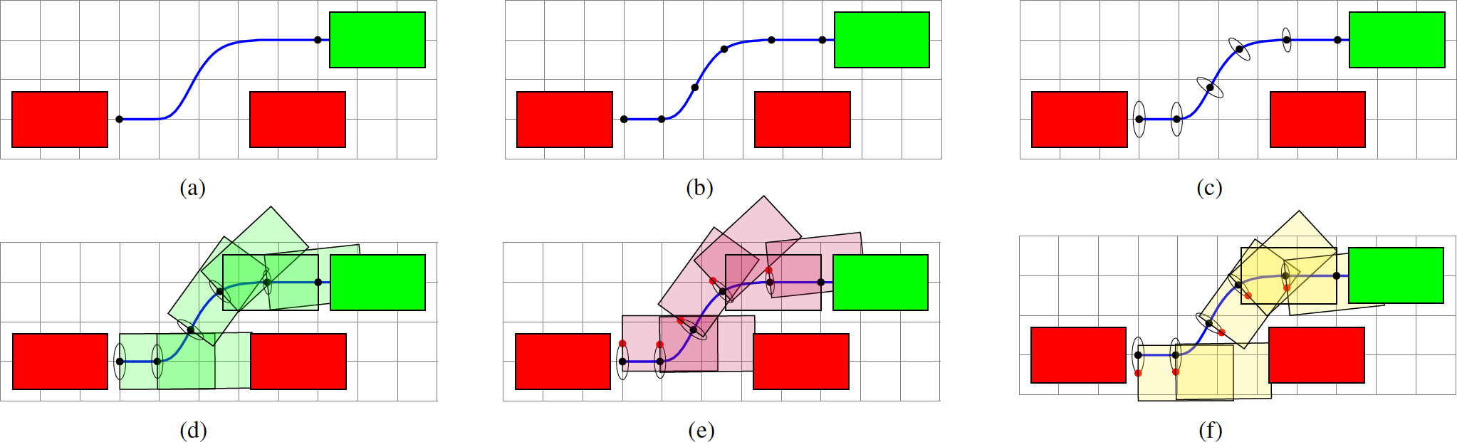
[a] A candidate trajectory is generated by selecting values of a, b, c for the Gompertz curve; [b] Candidate trajectory is re-parametrized to arc-length format and idealized, error-free sampling points (x(s), y(s)) are generated based on increments of sampling distance s_s; [c] Size evolution of slip-induced error ellipsoids at idealized, error-free sampling points is shown. Generation of these error ellipsoids are for slip pre-emption. Note that ellipsoid sizes are exaggerated here for increased visibility and clarity but otherwise we always use k₁ = 0.05 and k₂ = 0.02; [d] Vehicle orientation and steering angle at idealized, error-free sampling points are determined. Using kinematic model, idealized error-free motion of vehicle is simulated to check for collision. Collision occurs for this particular candidate trajectory; [e] Vehicle motion at one extremity of error ellipsoid at sampling point is simulated to check for collision. Collision occurs; [f] Vehicle motion at other extremity of error ellipsoid at sampling point is simulated to check for collision. Collision occurs. Since this candidate trajectory results in collision, a different candidate trajectory is selected in the next iteration.

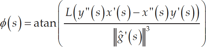
Subsequently, the magnitude of the steering angle(s) required to achieve the above vehicle orientation is determined by considering the trajectory curvature κ and robot dimension. Curvature κ is given by

κ (s) = \frac{‖ \hat{g}' (s) \times \hat{g} ″ (s) ‖}{{‖ \hat{g}' (s) ‖}^{3}}

(15)

The required steering angle is

ϕ (s) = atan (\frac{L (y ″ (s) x' (s) - x ″ (s) y' (s))}{{‖ \hat{g}' (s) ‖}^{3}})

(16)

for all s = {s_s, 2s_s, 3s_s, …, s_L}.

Thus, the required steering angles ϕ(s) that would realize the vehicle orientation θ(s) at the idealized, error-free point (x(s), y(s)) of the trajectory c(s) as determined by increments of the sampling distance s = {s_s, 2s_s, 3s_s, …, s_L} are determined. During real experiments, output of the vehicle odometry d_s is used to determine when the vehicle travels the distances s = {s_s, 2s_s, 3s_s, …, s_L} on the trajectory.

The final step is to simulate the vehicle motion on the trajectory considering slip and determine whether or not collision will occur. For this, eq. (1) is used to simulate the vehicle motion. Given that the vehicle dimensions are known and the vehicle orientations along the trajectory have been determined, the bounding box or four corners of the vehicle, as projected from the reference point x_c, y_c, at each of the sampling points (x(s), y(s)) can be determined. Collision is deemed to occur when the vehicle bounding box enroaches or is in close proximity to parked vehicles whose outer corners are perceptible in the scan data and whose hidden corners and edges can be extrapolated. In addition, not only is the idealized, error-free vehicle motion corresponding to idealized, error-free positions (x(s), y(s)) on the trajectory checked for collision, but the slip-induced, error-affected vehicle motion at both extremities of the error ellipsoid are also simulated to check for collisions. The entire process is summarized in the graphics of Fig. 9.

3.4 Optimization for Final Trajectory Parameter Deduction

Given a Gompertz curve with certain values of parameters {a, b, c}, the preceding section outlined the general procedure of determining values of the control input vector and simulating the vehicle motion to check for collisions while considering slip. The same procedure, together with additional constraints, is utilized iteratively for varying values of {b, c} to determine their best values (recall that parameter a has already been systematically determined using instantaneous scan data). Mathematically, this forms an optimization problem.

First, we define the necessary conditions and constraints. Let C = 0 denote the condition when there are no collisions. Let ϕ ∊ [−30°, 30°] be the constraint restraining the values of the required steering angles to the range imposed by the manufacturer. Both are hard constraints that need to be satisfied whenever enforced.

Given that parameter c is the more critical of the two parameters, the optimization scheme begins with fixing parameter b to a low value while optimizing c. We want the value of c that will minimize the slope of the Gompertz curve, and which simultaneously does not require steering angles beyond the maximum possible or result in collisions.

\underset{c}{\arg \min} \hat{g}' (a, b, c) | {C = 0, ϕ \in [- 30 °, 30 °]}

(17)

Figure 10.

Visualization of result of optimization scheme to determine the best values for b and c to realize a single-manoeuvre, parallel parking, Gompertz trajectory. The entire process of Fig. 9 is performed such that the trajectory satisfying two constraints is acquired: (1) that the optimized trajectory does not lead to a collision (2) that the steering angles required to realize the trajectory are within the range allowed.

For parameter b, we want the maximum value possible, using c_min found above, and subject to no collisions occurring.

\underset{b}{\arg \max} (\ln (\frac{\hat{g}}{a}) e^{- c_{\min} x}) | {C = 0}

(18)

If there are no solutions to either of the above, it implies that no collision-free, single-trajectory parallel-parking manoeuvre exists.

4. Results

Figure 10 gives a visualization of a simulation case of best trajectory generation during an optimization routine. Numerous different candidate trajectories are generated and tested by generating plausible values of b, c. For brevity, only two such candidate trajectories - in cyan and purple - are shown. By fulfilling the optimization constraints, the best trajectory to realize a single-manoeuvre, collision-free parallel parking - in blue - is generated.

Apart from such simulated results, real scan data was acquired using the real laser scanner on the car-like robot in an indoor carpark and the entire procedure was performed using the real sensor data. Figure 11 shows the real scan data of several test cases and the corresponding results. Different scenarios were tested and for each test case the location of the vehicle/sensor was varied with respect to the parking space in order to demonstrate the robustness of the algorithm in generating the correct trajectory despite the variations. In the scan plots, the location of the laser range scanner, installed on the midpoint of the vehicle rear end, is indicated by the • mark.

For the parking scenario of 11(a), generated trajectory parameters were a = 580, b = −50, c = −0.01. In Figure 11(b) it is seen that the length of the parking space has been extended and it is clearly evident that the trajectory generation procedure considered this by generating a smoother and relaxed turn to parallel-park inside of the parking space, thus generated value of c is smaller at c = −0.005. Moreover, now b = −40 assumes a bigger value imputed to the greater length of parking space available, implying that the vehicle commences alignment earlier compared to the first case.

Figures 11(c)–(d) similarly depict the second test case. The autonomous vehicle is located at different positions in (c) and (d) and it is seen how the resulting trajectory correctly predicts the parallel parking trajectory. It is seen in (d) that due to the proximity of the autonomous vehicle near the parked cars, the resulting Gompertz trajectory has a much sharper turn. For (c), parameters were a = 1000, b = −50, c = −0.006 and for (d) a = 450, b = −50, c = −0.02.

Figures 11(e)–(f) represent the final test case once again showing the trajectory generated for two different initial positions for the same parking scenario. For (e), parameters were a = 420, b = −40, c = −0.005 and for (f) a = 1200, b = −40, c = −0.005. The entire algorithm - scan data acquisition, parameter optimization and trajectory generation incurred less than 200ms of computation time for each of the test cases.

For the model vehicle, speeds of up to 30 cm/s have currently been tested and validated and this is therefore the putative range of safe speed. In the results shown in Fig. 13(a) to Fig. 13, 10(d), the trajectory end points were generated such that they are located perpendicularly to the midpoints of the detected frontal or rear edge of the vehicle parked behind with the distance to the vehicle being in the range 50cm to 80cm depending on the length of parking space available in each case. In Fig. 13(e) and Fig. 13(f), since there is a much longer parking space compared to Fig. 13(a)–(d), the destination point is chosen such that the distance from the vehicle to the rear wall was lm. It must be emphasized that the end points of all parking trajectories shown in Fig. 13 do not represent the final resting position of the vehicle. Instead, the generated end points of the trajectories are only intended to manoeuvre the vehicle inside the parking space. Once inside, the vehicle may adjust its spacing from the vehicle behind and vehicle in front as desired. It may be set as desired e.g equidistant from the vehicle behind and vehicle in front or a specific distance from the vehicle in front or vehicle in behind.

Figure 12 shows an example of a more detailed set of results for the case of Fig. 13(b). Here, not only the idealized, collision-free Gompertz trajectory is shown (in red) but in addition, the likely deviation in the form of error trajectories arising due to slip and odometery errors are also shown (in blue). Were the vehicle to slip or drift while tracing the ideal parking trajectory in red and end up following any path bounded by the two trajectories in blue, there would still be no collisions since the trajectories in blue have been tested for collisions during the optimization routine. The corresponding plots of steering angles for the results of Fig. 12 are presented in Fig. 13.

Finally, the starting position of the car need not be perfectly parallel to the other parked cars but small deviations from the parallel configuration is permissible since the required orientation of the car while traversing the Gompertz trajectory is calculated and that orientation is realized by steering by the appropriate steering angle. However, it must be noted that very large deviations are not desirable and may affect results since the vehicle will consume much space in changing orientation.

Figure 11.

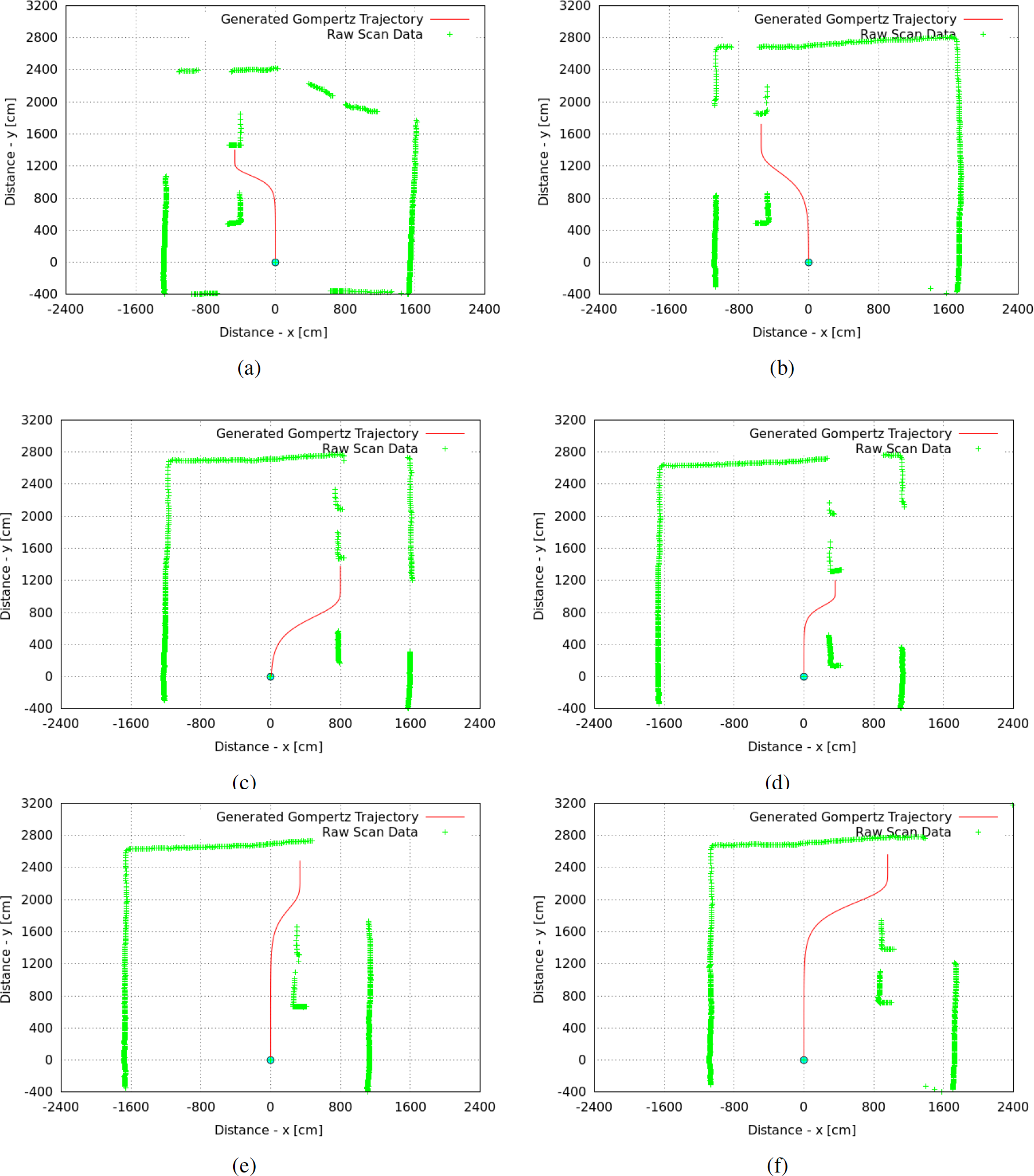
Gompertz trajectory for single-manoeuvre parallel parking generated in different cases during real experiments

Figure 12.

In addition to the ideal generated Gompertz trajectory (red), predicted error-affected trajectories that account for possible slip during parking are also shown (blue). All trajectories are collision-free.

Figure 13.

Corresponding plots of steering angles for Fig. 12

5. Conclusion

A new method of autonomously planning and executing parallel parking manoeuvres for autonomous vehicles was presented in this paper. First, the geometrical shape of the trajectory that realizes a parallel-parking manoeuvre in a single manoeuvre was identified in the form of a Gompertz curve. The merit of using the said curve as the trajectory of choice was in the flexibility of choosing the curve parameters to generate a collision free parking manoeuvre, based on the specific layout and dimension of a parking situation that the autonomous vehicle may encounter in the world. By parameter value variation, a safe and collision-free trajectory to generally any parallel parking situation can be realized.

During a real run, the exact parameter values are determined using the laser scanner. Thus in this approach no explicit user input is required, other than supervision.

Furthermore, the same trajectory can be used to exit the parking space. Subsequent to trajectory generation, the unit tangent vector at different points along the trajectory is determined. This unit tangent vector is intrinsically equivalent to the vehicle orientation at that point of the trajectory. Given the vehicle orientation, dimensions and odometry data, the steering angle that realizes a particular orientation at a particular point of the trajectory could be established. The method uses the trajectory in an arc-parametrized format together with the odometry data to determine at what point of the trajectory the vehicle is located. Implication of this approach is that the autonomous vehicle may travel at any arbitrary low speed while traversing the trajectory. To counter any slip errors originating from odometry readings, equations for the vehicle model were expanded to include include slip in both x and y directions using an error ellipsoid. Both simulations and real sensor data were used to demonstrate the validity of the proposed method.

References

Kasai

and Onoguchi

, “Lane Detection System for Vehicle Platooning using Multi-information Map”, 13th International IEEE Conference on Intelligent Transportation Systems, pp. 1350–1356, 19–22 Sept., 2010.

Kim

ZuWhan

, “Robust Lane Detection and Tracking in Challenging Scenarios”, IEEE Transactions on Intelligent Transportation Systems, Vol. 9, Issue 1, pp. 16–26, March 2008.

Qingquan

Chen

Long

Ming

Shaw

Shih-Lung

Nuchter

“A Sensor-Fusion Drivable-Region and Lane-Detection System for Autonomous Vehicle Navigation in Challenging Road Scenarios”, IEEE Transactions on Vehicular Technology, Vol. 63, Issue 2, pp. 540–555, Feb. 2014.

Fritsch

Kuhnl

and Kummert

, “Monocular Road Terrain Detection by Combining Visual and Spatial Information”, IEEE Transactions on Intelligent Transportation Systems, Vol. PP, Issue 99, pp. 1–11, 13 March 2014.

Greenhalgh

and Mirmehdi

, “Real-Time Detection and Recognition of Road Traffic Signs”, IEEE Transactions on Intelligent Transportation Systems, Vol. 13, Issue 4, pp. 1498–1506, Dec. 2012.

Gonzalez

Bergasa

L.M.

and Yebes

J.J

, “Text Detection and Recognition on Traffic Panels From Street-Level Imagery Using Visual Appearance”, IEEE Transactions on Intelligent Transportation Systems, Vol. 15, Issue 1, pp. 228–238, Feb. 2014.

Tao

and Ranganathan

, “Vehicle localization using road markings”, 2013 IEEE Intelligent Vehicles Symposium, pp. 1185–1190, 23–26 June 2013.

Lee

Joon-Yong

Kim

Mn-Soeng

Lee

Ju-Jang

, “Design of Fuzzy Controller for Car Parking Problem Using Evolutionary Multi-objective Optimization Approach”, IEEE International Symposium on Industrial Electronics, Montreal, pp. 329–334, July, 2006.

Wang

Zhao-Jian

Zhang

Jian-Wei

Huang

Ying-Ling

Zhang

Hui

Mehr

Aryan Saadat

, “Application of Fuzzy Logic for Autonomous Bay Parking of Automobiles”, International Journal of Automation and Computing, 8(4, pp. 445–451, November 2011.

10.

Suhr

Jae Kyu

Gi Jung

Bae

Kwanghyuk

Kim

Jaihie

, “Automatic free parking space detection by using motion stereo-based 3D reconstruction”, Machine Vision and Applications, 21, pp. 163–176, 2010.

11.

Seo

Young-Woo

Ratliff

Nathan

and Urmson

Chris

, “Self-Supervised Aerial Image Analysis for Extracting Parking Lot Structure”, Proceedings of International Joint Conference on Artificial Intelligence, July, 2009.

12.

Oyama

Kentaro

and Nonaka

Kenichiro

“Model Predictive Parking Control for Nonholonomic Vehicles using Time-State Control Form”, 2013 European Control Conference, pp. 458–465, July 17–19, Zurich, 2013.

13.

Tashiro

“Vehicle steering control with MPC for target trajectory tracking of autonomous reverse parking”, 2013 IEEE International Conference on Control Applications, pp. 247–251, 28–30 Aug. 2013.

14.

Zico Kolter

Plagemann

Christian

Jackson

David T.

Ng Sebastian Thrun

Andrew Y.

, “A Probabilistic Approach to Mixed Open-loop and Closed-loop Control, with Application to Extreme Autonomous Driving”, IEEE International Conference on Robotics and Automation, 2010.

15.

Kim

Dohyun

Song

Bongsob

, “Lateral Vehicle Control for Semi- Autonomous Valet Parking with Consideration of Actuator Dynamics”, International Journal of Control Science and Engineering 2(6): pp. 150–156, 2012.

16.

Pradalier

Vaussier

and Corke

, “Path planning for a Parking Assistance System: Implementation and Experimentation”, ACRA 2005.

17.

Zhang

Shuwen

Simkani

Zadeh

M.H

, “Automatic Vehicle Parallel Parking Design Using Fifth Degree Polynomial Path Planning”, IEEE Vehicular Technology Conference, pp. 1–4, 2011.

18.

Dudek

Gregory

and Jenkin

Michael

, “Computational Principles of Mobile Robotics”, pp. 47, Cambridge University Press, 2010.

19.

LaValle

Steven M.

, “Planning Algorithms”, Cambridge University Press, pp. 724, 2006.

20.

Jukić

Dragan

Kralik

Gordana

and Scitovski

Rudolf

, “Least-squares fitting Gompertz curve”, Journal of Computational and Applied Mathematics, Volume 169, Issue 2, pp. 359375, 15 August 2004.

21.

Madi

Mohsen

, “Closed-form expressions for the approximations of arclength parametrization for bezier curves”, Int. Journal of Applied Mathematics and Computing Science, Vol. 14, No. 1, pp. 33–41, 2004.

Application of Sigmoidal Gompertz Curves in Reverse Parallel Parking for Autonomous Vehicles

Abstract

Keywords

1. Introduction

2. Vehicle Model

3.3 Determination of Commanded Steering Angle(s)

References