Sage Journals: Discover world-class research

Abstract

The adaptive extended set-membership filter (AESMF) algorithm for robots' online modelling is today proposed for use in this field. Compared to the traditional ESMF, this novel filter method improves estimation accuracy under variable boundaries of unknown but bounded (UBB) process noise, which is often caused by the uncertainties of robotic dynamics. However, the applicability and stability of the AESMF method have not been tested in detail or demonstrated for real robotic systems. In this research, AESMF is applied for the actuator fault detections of a rotor-craft unmanned air vehicle (RUAV). The stability of AESMF is firstly analysed using mathematics and actuator healthy coefficients (AHC) are introduced for building the actuator failure model of RUAVs. AESMF is employed for the online boundary estimation of flight states and AHC parameters for fault tolerance control. Based on the proposed AESMF actuator fault estimation, flight experiments are conducted using a ServoHeli-40 RUAV platform and the flight results are compared with traditional ESMF and the adaptive extended Kalman filter (AEKF) in order to demonstrate its effectiveness, as well as for suggesting improvements for the actuator failure detection of RUAVs.

Keywords

RUAV actuator fault detection AESMF flight experiment investigation

1. Introduction

Fault detection (FD) techniques have been widely adopted by many applications to detect faults in sensors and actuators, for example, in the process industry [1], for unmanned ground vehicles (UGV) [2] and fixed-wing aircrafts [3]. The structure of the fault tolerant controller, for example, the H∞ controller [3, 4] and adaptive controller [5, 6] can be reconstructed to maintain the best control performance when a fault in systems is detected by FD techniques [7]. With the development of redundancy sensor technology, FD-based tolerance control of non-backup actuator failure is becoming ever more important for robotic systems such as RUAVs. However, few FD methods for RUAVs have been proposed [8, 9] for tolerance control use and actuator fault modelling, such as jammed collective pitch surface, dead engine, and pitch surface effectiveness loss, remain unsolved for RUAV systems because of uncertainty regarding dynamics.

Due to the difficulty of obtaining a high fidelity full envelope model for fault detection, the multi-mode modelling technique has been proposed for rotor- aircraft such as tilt-rotor aircraft XV-15 [11] and the helicopters BO-105 [12], UH-60 [13], R-50 [14] and X-Cell [15]. A mode-dependent actuator failure model, which is simplified according to a specific flight mode such as hovering, cruising, taking off and landing, can be used for the corresponding flight mode. However, the mode-dependent actuator failure model still suffers from at least one problem: difficulties in accommodating the mode transition dynamics (uncertainty dynamics) of RUAVs, which creates a time-varying process noise and additionally, cannot be described by certain prior knowledge.

Recently, improvements in the sequence estimation method have made actuator fault estimation for RUAVs more feasible [16]. Among the statistical system estimation methods, the Kalman filter is the best known [17, 18, 19]. This filter is also known as a state estimator that utilizes the statistical knowledge of both the system measurement noise and the process noise (e.g., white noise) and achieves optimal estimation by optimizing the minimum function of the estimation residuals. Furthermore, its algorithm representation includes predictions and updates, which is convenient in online applications. Hence, this method is widely used and has been developed to address nonlinear system estimation, thus extending its application field, for example, the extended Kalman filter (EKF) [20], the unscented Kalman filter (UKF) [21] and the derivative-free nonlinear Kalman filter [22].

However, these Kalman filters require statistical knowledge of the system measurement noise and of the process noise in general, or else it assumes that those noises meet some distributions in order to solve optimal problems in real applications such as RUAVs' fault detection [23, 24]. However, in reality, the system and environment noise characteristics are typically quite complicated, time varying and difficult to accurately measure. In particular, for RUAV systems, mechanical manufacturing accuracy, sensory noise and air flow disturbances will result in uncertain statistical noises. The mismatching of a noise's statistical characteristics will cause filter bias. Moreover, due to the Kalman filter's noise sensitivity, this bias is amplified and causes estimator instability. Therefore, many adaptive schemes, e.g., the adaptive unscented Kalman filter (AUKF) [25] have been introduced to Kalman estimators in order to achieve online noise estimation of the system's process noise distribution, as well as to compensate for filtering faults. However, statistical dependency and sensitivity of the Kalman estimator limit its system applications.

In most real systems, although noise's statistical characteristics are unknown, they can be assumed as an unknown-but-bounded (UBB) noise. Due to the listed defects of Kalman filtering, researchers have proposed a set-membership filter (SMF). Based on the UBB assumption, this filter provides a feasible state boundary by calculating the available set members. Thus, the estimation result is a viable state set rather than a single value. This viable state set describes possible ranges of the estimated parameters and makes sure that the real value falls within this set. Scholte and Campbell [26] expanded this ellipsoid algorithm into a nonlinear system and proposed an extended set-member filter (Extended SMF (ESMF)). This follows the same mechanism for Kalman filtering by linearizing nonlinear systems. However, the difference is that ESMF uses Taylor expansions rather than nonlinear system linearizations. This method changes inaccurate linearization into process noise in order to accomplish nonlinear system estimation. Yet to solve its numerical instability, poor real-time performance and difficulties in the tuning of the filter parameters, Zhou proposed a UD factorization-based extended set-membership filter [27]. This method represents and updates the envelope matrices using UD factorization. The method combines measurements in an updating strategy to improve the algorithm's stability and reduces its complexity, and has been used for online modelling of RUAVs by the authors in real aggressive flight control experiments [28].

However, the described method – the ESMF method – still requires the priori boundary information of the system noise for a RUAV's actuator estimations. Specifically, this algorithm needs to know the uncertain boundaries of the process and measurement noise. Generally, measurement noise depends on sensory accuracy. If the sensors work under normal conditions, the uncertain boundary does not drift. Therefore, measurement of the uncertain boundary from the sensor can be decided by analysing the sensor data; on the other hand, process noise arises from the mismatch between the system state space model and the system's real dynamics, such as mismatched parameters for RUAVs. Therefore, it is necessary to manually tune the boundary parameters, since the priori information of uncertain boundaries are unknown. Meanwhile, as prior knowledge is limited, manually setting the process noise's uncertain boundary may not include, or may well exceed the real process noise boundary. This will lead to the ESMF's estimated uncertain boundary being too large to deviate and will cause the filter to diverge during estimation of robots' UBB process noise, such as in the case of an RUAV's actuator fault. To solve this problem, the authors have proposed an AESMF [29] to address the process noise uncertain boundary issue for online robots' dynamics estimation. This method applies gradient descent optimization rules and conducts online calculation to obtain the minimal ellipsoid boundaries of the prediction error, which also ensures that the filter's health-index satisfies the working conditions for uncertainty dynamics. However, the stability condition and applicability of the AESMF are not verified by theory or real experiments, which limit its applications for robots' online modelling.

In this paper, firstly, the AHCs are introduced for building the model of RUAVs' actuator failures. Then, the AESMF is reviewed and applied to estimate both the states and the AHCs parameters in real time, and stability is demonstrated by a theorem. Finally, real flight experiments with the ServoHeli-40 RUAV test-bed are conducted and performance comparisons for fault modelling, among them AESMF, AUKF and AEKF, are discussed in order to verify their applicability for RUAVs' actuator fault detections.

Figure 1.

Body diagram of RUAV wit with respect to body coordination system

2. AHC Model for RUAVs' Actuator Faults

2.1 RUAV Dynamics Modelling

RUAV dynamics obey the Newton-Euler equation for rigid body in translational and rotational motion. Here, we considered a typical rigid RUAV in/near hover flight and the dynamic equation is conveniently described with respect to the body's coordination system, written is as:

(\begin{matrix} m I & 0_{3 \times 3} \\ 0_{3 \times 3} & I \end{matrix}) (\begin{matrix} {\dot{V}}^{B} \\ {\dot{Ω}}^{B} \end{matrix}) + (\begin{matrix} Ω^{B} \times m V^{B} \\ {\dot{Ω}}^{B} \times I Ω^{B} \end{matrix}) = (\begin{matrix} F_{e x t}^{B} \\ M_{e x t}^{B} \end{matrix})

(1)

where m ∊ R is the mass of the helicopter, V^B ∊ R^3×1 is the velocity vector for body frame, Ω ^B ∊ R^3×1 is the rotary speed vector for body frame, I ∊ R^3×3 is inertia matrix, $F_{e x t}^{B} \in R^{3 \times 1}$ is the force vector on the body and $M_{e x t}^{B} \in R^{3 \times 1}$ is the moment vector on the body.

The free body diagram of the RUAV with respect to the body's coordination system is as shown in Figure 1. By employing the lumped-parameter approach [30], which considers the RUAV as the composition made up of the main rotor, tail rotor, fuselage, horizontal stabilizer and vertical stabilizer, these components can be considered as the sources of forces and moments. The extern al force and moment, in hovering flight mode, can be written as:

\begin{array}{l} F_{e x t}^{B} = (\begin{matrix} X_{F} \\ Y_{F} \\ Z_{F} \end{matrix}) = (\begin{matrix} X_{M} \\ Y_{M} + Y_{T} \\ Z_{M} \end{matrix}) + R_{B} (\begin{matrix} 0 \\ 0 \\ m g \end{matrix}) \\ M_{e x t}^{B} = (\begin{matrix} L_{F} \\ M_{F} \\ N_{F} \end{matrix}) = (\begin{matrix} R_{M} + Y_{M} h_{M} + Z_{M} y_{M} + Y_{T} h_{T} \\ M_{M} + M_{T} - X_{M} h_{M} + Z_{M} l_{M} \\ N_{M} - Y_{M} l_{M} - Y_{T} l_{T} \end{matrix}) \end{array}

(2)

where R_B ∊ R^3×3 is the transition matrix between navigation frame and body frame, and the subscripts 'F' refers to the forces and moments in the helicopter's body frame. The forces X_T and Z_T, which are actuated by the tail rotor along the X-axis and Z-axis, are ignored as X_T, Z_T ≈ 0 for normal helicopters in (2). The forces X_V and Y_V, which are actuated by the tail stabilizer along the X-axis and Y-axis, can be ignored as X_V, Y_V ≈ 0 in hovering flight mode [31].

The forces and torques generated by the main rotor are controlled by T_M, a₁ and b₁. The tail rotor is considered a source of pure lateral force Y_T and anti-torque Q_T, which are controlled by T_T. Thus, the forces and moments can be expressed as [31]:

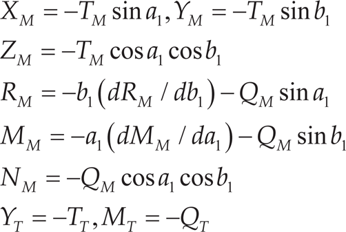
\begin{array}{l} X_{M} = - T_{M} \sin a_{1}, Y_{M} = - T_{M} \sin b_{1} \\ Z_{M} = - T_{M} \cos a_{1} \cos b_{1} \\ R_{M} = - b_{1} (d R_{M} / d b_{1}) - Q_{M} \sin a_{1} \\ M_{M} = - a_{1} (d M_{M} / d a_{1}) - Q_{M} \sin b_{1} \\ N_{M} = - Q_{M} \cos a_{1} \cos b_{1} \\ Y_{T} = - T_{T}, M_{T} = - Q_{T} \end{array}

(3)

where T_M, T_T are the force of the main rotor and tail rotor, a₁, b₁ are longitudinal and lateral flapping angle, Q_M, Q_T are the moments caused by the main rotor and tail rotor. Based on reference [32], T_i and Q_i, where i={T,M}, can be calculated as follows:

\begin{array}{l} T_{i} = \frac{R_{1 i}^{3} - R_{0 i}^{3}}{3} m_{3} θ_{c i} + \frac{m_{3} m_{6}}{2} (R_{1 i}^{2} - R_{0 i}^{2}) \\ - \frac{m_{3}}{8 π Ω_{i}^{2}} {\frac{2}{15 m_{2}^{2} θ_{c i}^{2}} ((3 m_{2} R_{1 i} θ_{c i} - 2 m_{5}) {(m_{2} R_{1 i} θ_{c i} + m_{5})}^{3 / 2} \\ - (3 m_{2} R_{0 i} θ_{c i} - 2 m_{5}) {(m_{2} R_{0 i} θ_{c i} + m_{5})}^{3 / 2})} \\ Q_{i} = n_{1} n_{7} \frac{R_{1 i}^{3} - R_{0 i}^{3}}{3} - \frac{n_{1} n_{9}}{2} (R_{1 i}^{3} - R_{0 i}^{3}) + \frac{c_{d} n_{1}}{4} (R_{1 i}^{4} - R_{0 i}^{4}) \\ + \frac{2 n_{1} n_{8}}{105 m_{4}^{3}} {(15 m_{4}^{2} R_{1 i}^{2} - 12 m_{4} m_{5} R_{1 i} + 8 m_{5}^{2}) {(m_{4} R_{1 i} + m_{5})}^{3 / 2} \\ - (15 m_{4}^{2} R_{0 i}^{2} - 12 m_{4} m_{5} R_{0 i} + 8 m_{5}^{2}) {(m_{4} R_{0 i} + m_{5})}^{3 / 2}} \\ + \frac{2 n_{1} n_{10}}{15 m_{4}^{3}} {(3 m_{2} R_{1 i} - 2 m_{5}) {(m_{2} R_{1 i} + m_{5})}^{3 / 2} \\ - (3 m_{2} R_{0 i} - 2 m_{5}) {(m_{2} R_{0 i} + m_{5})}^{3 / 2}} \end{array}

(4)

where

\begin{array}{l} m_{1} = \frac{Ω_{i}}{2} a_{i} b_{i} c_{i} + 4 π V_{c} m_{2} = 8 π Ω_{i}^{2} a_{i} b_{i} c_{i} \\ m_{3} = \frac{ρ}{2} Ω_{i} a_{i} b_{i} c_{i} + 4 π V_{c} m_{4} = m_{2} θ_{c i} \\ m_{5} = m_{1}^{2} - \frac{V_{c} m_{2}}{Ω_{i}} m_{6} = \frac{1}{Ω_{i}} (\frac{m_{1}}{8 π} - V_{c}) \\ n_{1} = \frac{ρ}{2} Ω_{i}^{2} b_{i} c_{i} n_{2} = V_{c} - \frac{m_{1}}{8 π} \\ n_{3} = \frac{a_{i}}{{(8 π Ω_{i})}^{2}} n_{4} = m_{1}^{2} + m_{5} \\ n_{5} = \frac{a V_{c}}{4 π Ω_{i}^{2}} n_{6} = a_{i} {(\frac{V_{c}}{Ω_{i}})}^{2} \\ n_{7} = \frac{a_{i} θ_{c i}}{Ω_{i}} n_{2} - n_{3} m_{4} n_{8} = \frac{a θ_{c i}}{8 π Ω_{i}} \\ n_{9} = n_{3} n_{4} - n_{5} m_{1} + n_{6} n_{10} = 2 m_{1} n_{3} - n_{5} \end{array}

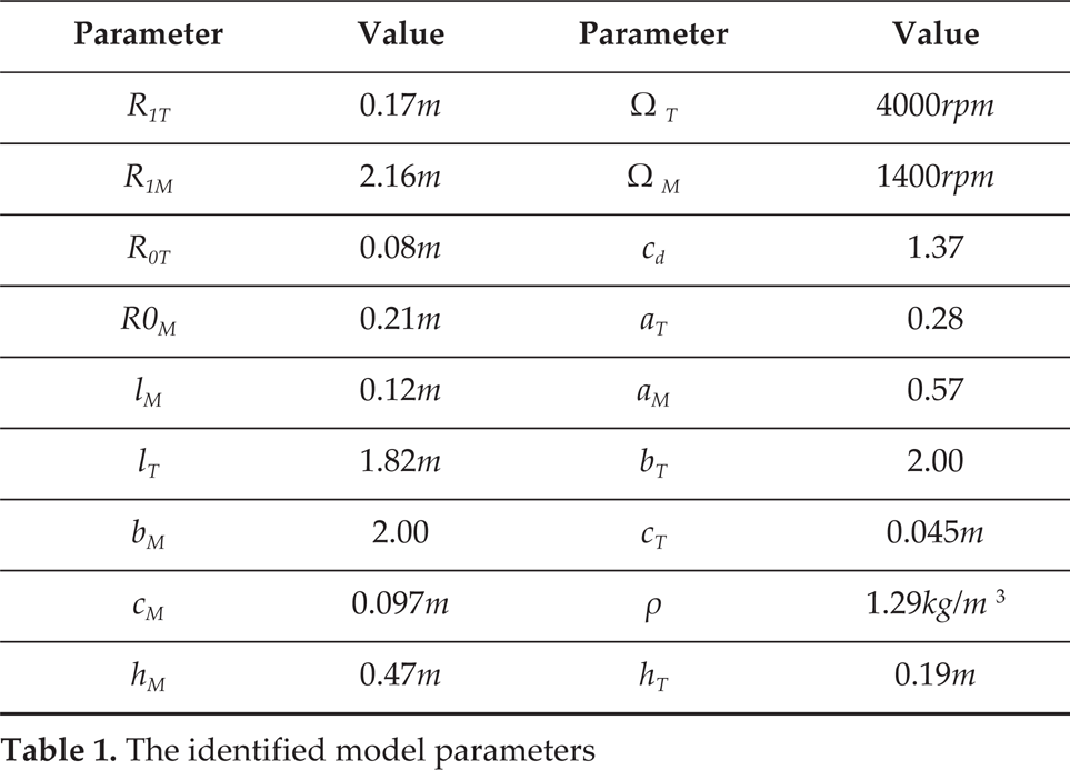
where R_1T is the radius of the tail rotor, R_1M is the radius of the main rotor, R_0T is the inner radius of the tail rotor, R_0M is the inner radius of the main rotor, Ω_T is the rotation speed of the tail rotor, Ω_M is the rotation speed of the main rotor, b_M is the number of the main rotor's blade, b_T is the number of the tail rotor's blade, c_d is the thrust coefficient of the main rotor, a_T is the gradient of lift curve for the tail rotor, a_M is the gradient of the lift curve for the main rotor, ρ is the density of air, c_T is the width of the tail rotor, c_M is the width of the main rotor, θ_cM is the collective pitch angle of the main rotor, θ_cT is the collective pitch angle of the tail rotor and V_c is the vertical speed of RUAV. All of the above parameters, which can be measured or identified, are shown in Table 1.

Table 1.

The identified model parameters

Parameter	Value	Parameter	Value
R_1T	0.17m	Ω_T	4000rpm
R_1M	2.16m	ΩM	1400rpm
R_0T	0.08m	c_d	1.37
R0_M	0.21m	a_T	0.28
ι_M	0.12m	a_M	0.57
ι_T	1.82m	b_T	2.00
b_M	2.00	c_T	0.045m
c_M	0.097m	ρ	1.29kg/m³
h_M	0.47m	h_T	0.19m

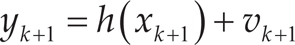
Let control output U_out = (θ_cM θ_cT a₁ b₁), then we can obtain a RUAV dynamics model based on (1) ∼ (4), which has the following state-space structure:

{\begin{cases} \dot{x} = f (x, U_{o u t}) \\ y = x \end{cases}

(5)

where x = (V^BT Ω^BT)^T is the state vector, y is the measurement vector and f(x, U_out) is a non-linear mapping function.

2.2 Actuator Failure Model with AHCs

The actuator failures of the RUAV include the control surface jam, control surface bias and partial loss in the actuator effectiveness [33]. Define U_in as the inputs (desired surface position) and Uout as the outputs (real control surface position) of the actuators. The fault tolerant architecture then assumes the following actuator model:

U_{o u t} = d i a g {Γ_{f}^{T}} U_{i n} + Δ_{f}

(6)

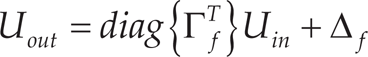
where

Γ_{f} = {(γ_{1}, …, γ_{4})}^{T} Δ_{f} = {(δ_{1}, …, δ_{4})}^{T}

and where γ_i and δ_i are the proportional effectiveness and failure bias of the i-th actuator's AHCs with i = {1, 2, 3, 4} and the range of Uin is defined as in [0,1]. Definition (6) means that control surface position bias is Δ_f and (1 1 1 1)^T−Γ_f loss occurs in actuator effectiveness. For example, if γ₂ = 0, this means the tail rotor is jammed at position δ₂; if δ₂ = 0, this means the tail rotor experiences 1-δ₂ loss in effectiveness.

The AHC expression (6) aims to make the proportional effectiveness and failure bias of actuators parametric, so that a fault model can be built using online estimation [34]. The estimation model will be built in the following part.

2.3 States and AHCs' Parameter Joint Estimation Model

To estimate the AHCs' parameters, we built an extended dynamics model for the joint estimation of states and parameters of RUAVs. To do this, AHCs and state vectors were concatenated into a single augmented state vector at discrete time k:

x_{k}^{a} = {(\begin{matrix} V^{B T} & Ω^{B T} & Γ_{f}^{T} & Δ_{f}^{T} \end{matrix})}^{T}

(7)

Thus, estimation was done recursively by writing the dynamics (1 ∼ 6) in discrete equations for the joint state as the following non-linear structure:

{\begin{cases} x_{k}^{a} = \tilde{f} (x_{k - 1}^{a}, U_{i n,}_{k}) + w_{k}^{a} \\ y_{k} = \tilde{h} (x_{k}^{a}) + v_{k} \end{cases}

(8)

where $\tilde{f} (x_{k}^{a}, U_{i n, k}) = (f {(x_{k}, U_{i n, k})}^{T}, Γ_{f, k}^{T}, Δ_{f, k}^{T})$ is a non-linear mapping function, $w_{k}^{a} \in R^{14 \times 1}$ is the UBB process noise and v_k ∊ R^6×1 is the measurement noise, which can be calibrated based on the accuracy of the sensors on RUAVs.

The AHCs' joint estimation has advantages over some existing modelling techniques, where only proportional loss in effectiveness has been considered. However, the distribution of $w_{k}^{a}$ cannot be decided, because of the UBB characteristics and Kalman-type filter, e.g., EKF, which is often used in FD but cannot be used for the estimation of AHCs, and where a set-membership filter is a better estimation method for this condition. Furthermore, the boundary $w_{k}^{a}$ is variable according to flight modes and mechanical parameters; therefore, it cannot be exactly selected offline. Thus, in this instance, AESMF may be more useful than traditional ESMF for estimations.

Hence, in the flowing parts, the AESMF method will be reviewed first and its stability demonstrated by a theorem. Following on, the AESMF will be used to estimate the AHC actuator fault model (8) and compare it to traditional ESMF and EKF via experiments.

3. AESMF Review and Stability Analysis

3.1 AESMF Algorithm Review

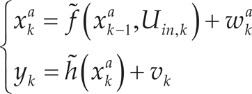
The nonlinear system considered here is expressed as:

x_{k + 1} = f (x_{k}) + w_{k}

(9)

y_{k + 1} = h (x_{k + 1}) + v_{k + 1}

(10)

where x_k ∊ Rⁿ and y_k+1 ∊ R^m are the state and measurement vectors, respectively, f() and h() are nonlinear C² functions, w_k ∊ Rⁿ and v_k ∊ R^m are the process and measurement noise vectors, respectively, and they meet the necessary conditions:

w_{k} \in E (0_{n \times 1}, Q_{k}), v_{k + 1} \in E (0_{m \times 1}, R_{k + 1})

where E(a, P) stands for an ellipsoid set as:

E (a, P) = {x \in R^{n} : {(x - a)}^{T} P^{- 1} (x - a) \leq 1}

where a is the centre, x is any point within the ellipsoid and P is a positive-definite matrix.

The initial estimation ellipsoid is defined as

x_{0} \in E ({\hat{x}}_{0}, P_{0})

where ${\hat{x}}_{0}$ and P₀ stand for the initial estimation of ellipsoid centre and envelope matrix, respectively. At time k, the estimated ellipsoid is defined as

E_{k} = E ({\hat{x}}_{0}, P_{k}) .

Set $q_{k}^{i} \in R$ as the i-th diagonal element in Q_k at time k, ${\hat{q}}_{k}^{i} \in R$ as the i-th diagonal element in ${\hat{Q}}_{k}$ at time k, ${\hat{Q}}_{k}$ as the estimation of Q_k at time k; then, at time k+1, k=0, 1, 2,…, the AESMF algorithm [29] can be summarized as follows:

Intial conditions:

{\hat{q}}_{0}^{i} = q_{0}^{i}, Q_{0} = d i a g {{\hat{q}}_{0}^{1}, {\hat{q}}_{0}^{2}, …, {\hat{q}}_{0}^{n}}, {\hat{P}}_{0} = P_{0}

(11)

Construction of the noise boundaries at times k+1:

{\begin{cases} X_{k}^{i} = [\begin{matrix} {\hat{x}}_{k}^{i} - \sqrt{P_{k}^{i, i}} & , {\hat{x}}_{k}^{i} + \sqrt{P_{k}^{i, i}} \end{matrix}] \\ X_{R_{2}} = \frac{1}{2} diag (\underset{n}{\underset{︸}{X_{k}^{T} - {\hat{x}}_{k}, X_{k}^{T} - {\hat{x}}_{k}, …, X_{k}^{T} - {\hat{x}}_{k}}}) \\ • (H e s_{1}, …, H e s_{n}) (X_{k} - {\hat{x}}_{k}) \\ {[{\bar{Q}}_{k}]}_{R_{k}}^{i, i} = 2 {(X_{R_{2}})}^{2}, {[{\bar{Q}}_{k}]}_{R_{k}}^{i, j} = 0_{n \times 1} (i \neq j) \\ β_{Q_{k}} = \sqrt{Tr (Q_{k})} / (\sqrt{Tr ({\bar{Q}}_{k})} + \sqrt{Tr (Q_{k})}) \\ {\hat{Q}}_{k} = {\bar{Q}}_{k} / (1 - β_{Q_{k}}) + Q_{k} / β_{Q_{k}} \end{cases}

(12)

where X_R2 is the interval of the Lagrange remainder of f(x_k), $X_{k}^{i}$ is the interval of x_k and Hes_i, i = 1, 2,…, n are the i-th Hessian matrix of nonlinear function f(x_k).

Time update at time k+1:

{\begin{cases} {\hat{x}}_{k + 1, k} = f ({\hat{x}}_{k}) \\ β_{k} = \sqrt{Tr ({\hat{Q}}_{k})} / (\sqrt{Tr (Φ_{k} P_{k} Φ_{k}^{T})} + \sqrt{Tr ({\hat{Q}}_{k})}) \\ P_{k + 1, k} = Φ_{k} P_{k} / (1 - β_{k}) Φ_{k}^{T} + {\hat{Q}}_{k} / β_{k} \end{cases}

(13)

where $Φ_{k} = \partial f (x_{k}) / \partial x_{k} |_{x_{k} = {\hat{x}}_{k}}$ is the Jacobian matrix of model (9).

Measure update at time k+1:

{\begin{cases} ρ_{k} = \sqrt{r_{m}} / (\sqrt{p_{m}} + \sqrt{r_{m}}) \\ W_{k} = H_{k + 1} P_{k + 1, k} H_{k + 1}^{T} / (1 - ρ_{k}) + {\hat{R}}_{k + 1} / ρ_{k} \\ K_{k + 1} = P_{k + 1, k} H_{k + 1}^{T} W_{k}^{- 1} / (1 - ρ_{k}) \\ {\hat{x}}_{k + 1} = {\hat{x}}_{k + 1, k} + K_{k + 1} [y_{k + 1} - h ({\hat{x}}_{k + 1, k})] \\ {\bar{P}}_{k + 1} = \frac{P_{k + 1, k}}{1 - ρ_{k}} - \frac{P_{k + 1, k}}{1 - ρ_{k}} H_{k + 1}^{T} W_{k}^{- 1} H_{k + 1} \frac{P_{k + 1, k}}{1 - ρ_{k}} \\ δ_{k} = 1 - {[y_{k + 1} - h ({\hat{x}}_{k + 1, k})]}^{T} W_{k}^{- 1} [y_{k + 1} - h ({\hat{x}}_{k + 1, k})] \\ P_{k + 1} = δ_{k} {\bar{P}}_{k + 1} \end{cases}

(14)

where $H_{k + 1} = \partial h (x_{k + 1}) / \partial x_{k + 1} | x_{k + 1} = {\hat{x}}_{k + 1, k}_{}$ is the Jacobian matrix of model (10) and p_mr_m are maximum singular values of the matrix $H_{k + 1} P_{k + 1, k} H_{k + 1}^{T}$ and R_k+1, respectively.

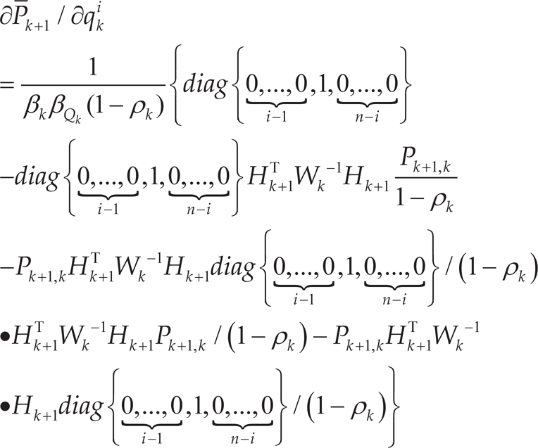
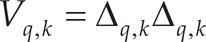
Process noise boundaries update at time k+1:

{\begin{cases} {\hat{q}}_{k + 1}^{i} = {\hat{q}}_{k}^{i} - Δ T • η_{k} \\ • t r {(1 - 2 δ_{k}) (\partial δ_{k} / \partial q_{k}^{i}) {\bar{P}}_{k + 1} + (1 - δ_{k}) δ_{k} (\partial {\bar{P}}_{k + 1} / \partial q_{k}^{i})} \\ Q_{k + 1} = d i a g {{\hat{q}}_{k + 1}^{1}, {\hat{q}}_{k + 1}^{2}, …, {\hat{q}}_{k + 1}^{n}} \end{cases}

(15)

where tr{•} is the track of a matrix and

\begin{array}{l} \partial {\bar{P}}_{k + 1} / \partial q_{k}^{i} \\ = \frac{1}{β_{k} β_{Q_{k}} (1 - ρ_{k})} {d i a g {\underset{i - 1}{\underset{︸}{0, …, 0}}, 1, \underset{n - i}{\underset{︸}{0, …, 0}}} \\ - d i a g {\underset{i - 1}{\underset{︸}{0, …, 0}}, 1, \underset{n - i}{\underset{︸}{0, …, 0}}} H_{k + 1}^{T} W_{k}^{- 1} H_{k + 1} \frac{P_{k + 1, k}}{1 - ρ_{k}} \\ - P_{k + 1, k} H_{k + 1}^{T} W_{k}^{- 1} H_{k + 1} d i a g {\underset{i - 1}{\underset{︸}{0, …, 0}}, 1, \underset{n - i}{\underset{︸}{0, …, 0}}} / (1 - ρ_{k}) \\ • H_{k + 1}^{T} W_{k}^{- 1} H_{k + 1} P_{k + 1, k} / (1 - ρ_{k}) - P_{k + 1, k} H_{k + 1}^{T} W_{k}^{- 1} \\ • H_{k + 1} d i a g {\underset{i - 1}{\underset{︸}{0, …, 0}}, 1, \underset{n - i}{\underset{︸}{0, …, 0}}} / (1 - ρ_{k})} \end{array}

(16)

\begin{array}{l} \frac{\partial δ_{k}}{\partial q_{k}^{i}} = - {(β_{k} β_{Q_{k}} (1 - ρ_{k}))}^{- 1} {[y_{k + 1} - h ({\hat{x}}_{k + 1, k})]}^{T} W_{k}^{- 1} \\ • H_{k + 1} d i a g {\underset{i - 1}{\underset{︸}{0, …, 0}}, 1, \underset{n - i}{\underset{︸}{0, …, 0}}} H_{k + 1}^{T} W_{k}^{- 1} {[y_{k + 1} - h ({\hat{x}}_{k + 1, k})]}^{T} \end{array}

(17)

where, i = 1, 2, ‥, n and j = 1, 2, ‥, n. ΔT is the sampling time, and η_k ∊ R, which is selected by hand, is the parameter for converge rate.

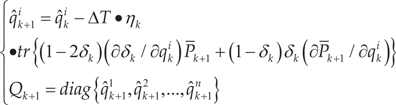
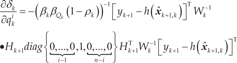
Since this adaptive strategy for process noise boundary is based on gradient descent (GD), according to step 5), this type of AESMF is referred to as GD-ESMF in following experiments. For the details about the GD-ESMF algorithm, please refer to [29].

3.2 Stability Analysis

Theorem: for system model (9) and (10), if the following conditions are satisfied:

Existing $\bar{a}, \bar{c} \in R$ , make $‖ A_{k} ‖ \leq \bar{a}$ and $‖ C_{k} ‖ \leq \bar{c}$

Initial process noise ellipsoid satisfies:

‖ (q_{0}^{i} - q^{i}) / q_{0}^{i} ‖ < q^{i} / w_{k}^{i} w_{k}^{i}

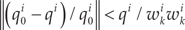
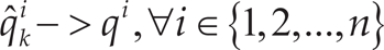
then, AESMF is stable and there is:

{\hat{q}}_{k}^{i} - > q^{i}, \forall i \in {1, 2, …, n}

proof:

\begin{array}{l} {\hat{q}}_{k + 1}^{i} = {\hat{q}}_{k}^{i} - Δ T • η_{k} • t r {\partial (1 - δ_{k}) P_{k + 1} / \partial q_{k}^{i}} \\ = {\hat{q}}_{k}^{i} + Δ T • η_{k} • \frac{\partial δ_{k}}{\partial q_{k}^{i}} t r {P_{k + 1}} \\ - Δ T • η_{k} • (1 - δ_{k}) • t r {\frac{\partial P_{k + 1}}{\partial q_{k}^{i}}} \end{array}

Let $Δ_{q, k} = q^{i} - {\hat{q}}_{k}^{i}$ then

\begin{array}{l} Δ_{q, k + 1} = q^{i} - {\hat{q}}_{k + 1}^{i} \\ = q^{i} - {\hat{q}}_{k}^{i} - Δ T • η_{k} • (\partial δ_{k} / \partial q_{k}^{i}) t r {P_{k + 1}} \\ + Δ T • η_{k} • (1 - δ_{k}) • t r {\partial P_{k + 1} / \partial q_{k}^{i}} \\ = Δ_{q, k} + Δ T • η_{k} • ((1 - δ_{k}) \\ • t r {\partial P_{k + 1} / \partial q_{k}^{i}} - \frac{\partial δ_{k}}{\partial q_{k}^{i}} t r {P_{k + 1}}) \end{array}

Make the Lyapunov function as:

V_{q, k} = Δ_{q, k} Δ_{q, k}

According to the proof of reference theorem [26], the following inequalities exist:

‖ P_{k} ‖ \leq \bar{p}, ‖ K_{k} ‖ \leq \bar{k}

where $\bar{p} \in R$ is the supremum of $‖ P_{k} ‖$ , $\bar{k} \in R$ is the supremum of $‖ K_{k} ‖$ . According to condition 1), there is

\begin{array}{l} V_{q, k + 1} - V_{q, k} = Δ_{q, k + 1} Δ_{q, k + 1} - Δ_{q, k} Δ_{q, k} \\ = (2 q^{i} - 2 {\hat{q}}_{k + 1}^{i} + Δ T • η_{k} • ((1 - δ_{k}) • t r {\frac{\partial P_{k + 1}}{\partial q_{k}^{i}}} \\ - \frac{\partial δ_{k}}{\partial q_{k}^{i}} t r {P_{k + 1}})) Δ T • η_{k} • ((1 - δ_{k}) • t r {\partial P_{k + 1} / \partial q_{k}^{i}} \\ - (\partial δ_{k} / \partial q_{k}^{i}) t r {P_{k + 1}}) \\ \leq - {\frac{1}{β_{k} β_{Q_{k}} (1 - ρ_{k}) {\bar{p}}^{2} (\bar{p} + {\bar{a}}^{2} q^{i})} ‖ Δ_{q, k} ‖ \\ + 2 {‖ Δ_{q, k} ‖}^{2} (\bar{a} + \bar{a} \bar{k} \bar{c}) ‖ Δ_{q, k} ‖} \\ {q^{i} / w_{k}^{i} w_{k}^{i} - ‖ (q_{0}^{i} - q^{i}) / q_{0}^{i} ‖} {w_{k}^{i} w_{k}^{i} / q^{i} - q^{i} / w_{k}^{i} w_{k}^{i}} \end{array}

and qⁱ is the boundary of process noise $w_{k}^{i}$ there must be $w_{k}^{i} w_{k}^{i} / q^{i} < 1$ so, there is:

w_{k}^{i} w_{k}^{i} / q^{i} - q^{i} / w_{k}^{i} w_{k}^{i} > 0

According to condition 2), there is:

\begin{array}{l} V_{q, k + 1} - V_{q, k} = Δ_{q, k + 1} Δ_{q, k + 1} - Δ_{q, k} Δ_{q, k} . \\ \leq - {\frac{1}{β_{k} β_{Q_{k}} (1 - ρ_{k}) {\bar{p}}^{2} (\bar{p} + {\bar{a}}^{2} q^{i})} ‖ Δ_{q, k} ‖ + 2 {‖ Δ_{q, k} ‖}^{2} (\bar{a} + \bar{a} \bar{k} \bar{c}) ‖ Δ_{q, k} ‖} \\ {q^{i} / w_{k}^{i} w_{k}^{i} - ‖ (q_{0}^{i} - q^{i}) / q_{0}^{i} ‖} {w_{k}^{i} w_{k}^{i} / q^{i} - q^{i} / w_{k}^{i} w_{k}^{i}} \end{array}

Because $0 < ρ_{k} < 1$ , $β_{k} > 0$ , $β_{Q_{k}} > 0$ , $\bar{a} > 0$ , $\bar{k} > 0$ , $\bar{c} > 0$ , $\bar{p} > 0$ and $q^{i} > 0$ , there is:

\frac{1}{β_{k} β_{Q_{k}} (1 - ρ_{k}) {\bar{p}}^{2} (\bar{p} + {\bar{a}}^{2} q^{i})} ‖ Δ_{q, k} ‖ + 2 {‖ Δ_{q, k} ‖}^{2} (\bar{a} + \bar{a} \bar{k} \bar{c}) ‖ Δ_{q, k} ‖ > 0.

According to condition 2), as $‖ (q_{0}^{i} - q^{i}) / q_{0}^{i} ‖ < q^{i} / w_{k}^{i} w_{k}^{i}$ , there is:

q^{i} / w_{k}^{i} w_{k}^{i} - ‖ (q_{0}^{i} - q^{i}) / q_{0}^{i} ‖ > 0.

Consider $w_{k}^{i} w_{k}^{i} / q^{i} - q^{i} / w_{k}^{i} w_{k}^{i} > 0$ , then,

\begin{array}{l} V_{q, k + 1} - V_{q, k} = Δ_{q, k + 1} Δ_{q, k + 1} - Δ_{q, k} Δ_{q, k} \\ \leq - {\frac{1}{β_{k} β_{Q_{k}} (1 - ρ_{k}) {\bar{p}}^{2} (\bar{p} + {\bar{a}}^{2} q^{i})} ‖ Δ_{q, k} ‖ + 2 {‖ Δ_{q, k} ‖}^{2} (\bar{a} + \bar{a} \bar{k} \bar{c}) ‖ Δ_{q, k} ‖} \\ {q^{i} / w_{k}^{i} w_{k}^{i} - ‖ (q_{0}^{i} - q^{i}) / q_{0}^{i} ‖} {w_{k}^{i} w_{k}^{i} / q^{i} - q^{i} / w_{k}^{i} w_{k}^{i}} < 0 \end{array}

Hence, GD rules (39) are stable and:

Δ_{q, k} - > 0, k - > \infty

Which means

{\hat{q}}_{k}^{i} - > q^{i}, \forall i \in {1, 2, …, n} .

In the following parts, a simulation and flight experiments are both conducted to compare performance among AESMF, AUKF and AEKF for actuator fault estimations.

4. Simulations and Flight Experiments

To test the performance of the proposed AESMF (10∼16) for actuator fault estimation based on AHCs (5 and 6), firstly, a Servoheli-40 RUAV test-bed is introduced and the parameters of model (5) are identified, based on the collected flight data from the ServoHeli-40 by remote control. Then, based on the AHC model (6), the estimation methods such as AESMF, AUKF and AEKF are all applied for estimation. The results are compared in both the simulation and real flight experiments.

4.1 Flight Test Platform

All flight tests were conducted on the Servoheli-40 RUAV, which was developed in our laboratory. It is equipped with a 3-axis gyro, a 3-axis accelerometer, a compass and a GPS. The sensory data can be sampled and stored onto an SD card through an onboard DSP. More details of this experimental platform can be found in [35]. The measurement accuracy of attitude is 0.1 degrees and the measurement accuracy of velocity is 0.01 m/s; measurement accuracy of the position is 0.1 m and the measurement accuracy of acceleration is 0.01 m/s². Figure 2 shows the test-bed RUAV. The parameters of model (8) in hovering mode are identified by the frequency response method [36] and are listed in Table 1. The matching accuracy is shown in Figure 3. The following experiments were conducted based on the there identified dynamics model.

Figure 2.

SERVOHELI-40 small-size RUAV

Figure 3.

The results of the model accuracy test

4.2 Actuator Failures Estimation Simulations

The proposed failure estimation scheme was firstly tested using the ServoHeli-40 mathematical model, which was identified with the real flight data from the hovering experiments, as above. Here, we combined the fault detection algorithm with a feedback linearization control scheme to perform the flights in our hardware-in-the-loop (HIL) environment [37], as shown in Figure 4; this was conducted due to the danger of actuator faults in real flight.

Figure 4.

Hill environment for RUAV simulations

AUKF-based, the traditional ESMF-based and proposed AESMF-based failure estimation schemes were tested together under coupled actuator failures as:

{\begin{cases} γ_{1, 4} = 100 %, δ_{1, 4} = 0, k < 100 \\ γ_{1} = 40 %, δ_{1} = 0.15, k \geq 100 \\ γ_{4} = 0 %, δ_{4} = 0.15, k \geq 100 \end{cases} .

This means that the roll control surface was 60% loss and its position bias was 15%, and the tail rotor control surface was jammed at a 15% position. Initial process noise ellipsoidal boundary Q0 was set larger than the real boundary as:

Q_{0} = 10^{- 2} • 0.25 I_{14 \times 14} .

To test the advantage of ESMF-based methods in fault parameters' boundary estimation, compared to AUKF (3σ bound), the real process noise w_k was generated as coloured ellipsoidal noise, which often happens in real practice as:

{(w_{k} - 0.01 • (\begin{matrix} 1 & 1 & … & 1 \end{matrix}))}^{T} Q_{0}^{- 1} (w_{k} - 0.01 • (\begin{matrix} 1 & 1 & … & 1 \end{matrix})) \leq 1 / 2

Figure 5 shows the AHC-bound estimation comparison among AUKF, ESMF and proposed GD-ESMF. It can be seen that AUKF's AHC boundaries is unable to cover the real fault parameters, because of the coloured process noise. AUKF requires some distribution noise; therefore, estimation is biased under coloured ellipsoidal noise. ESMF and the proposed GD-ESMF method for AHCs boundaries both can cover true value during estimation; however, the true values are not at the middle of the estimated ellipsoidal bound for ESMF, because of the biased noise. The proposed GD-ESMF obtains the best estimated boundaries for AHCs, because GD strategy regulates the ellipsoidal boundaries to real boundaries and the true values are almost at the middle of its ellipsoidal boundaries.

Figure 5.

AUKF, ESMF, GD-ESMF and AHC estimation performance comparisons under coloured noise

The above is shown by taking a simulation where the proposed GD-ESMF-based actuator fault modelling for RUAVs has the best estimation performance of uncertainty boundaries and comparing it with AUKF and ESMF. However, because of its lowest computation cost among the three methods, adaptive KF-based estimators are often used for fault detection, although its performance is worse than GD-ESMF under the uncertainty dynamics in the above simulation. However, the adaptive KF-based method cannot work as a proper estimator for the fault model based control of RUAVs; this conclusion will be verified by a real flight test in the following part.

4.3 Flight Test of Actuator Failures Estimation

In this part, the AESMF is compared with an adaptive KF-based estimator for the online fault model based control of RUAVs in flight experiments. The computational burden of AUKF is large, such as the root mean square matrix, which cannot be realized efficiently in the embedded flight controller under C++ programing. Thus, AEKF was instead adopted for the comparisons with proposed GD-ESMF in real flight experiments in this part. To test the AEKF and proposed GD-ESMF estimation for actuator fault, the following experiment was designed using a ServoHeli-40 RUAV platform.

As shown in Figure 6, the flight system's structure includes an onboard part and a ground part. The onboard part includes the flight controller, fault generator and steering gears, and the ground part includes the remote controller for the pilot and the ground station. In the following experiments, a remote controller is used to have the ServoHeli-40 take on/off. There is a button on the remote controller for the pilot that can change the flight mode between manual control and autonomous control. For flight safety, the pilot can change the flight mode into manual mode at any time during the flight. The ground station can transmit the actuator fault parameters in model (6) to the onboard fault generator, which actuates the steering gears to simulate the actuators' faults, based on the parameters in the following tests. The electronic devices, such as the flight controller, onboard fault generator and ground station, were all developed by the authors for experimental use. All of the hardware and software were also created by the authors, so that the model and control algorithm could be freely embedded by C++ programing. The details of the flight control system can be referred to in [35].

Figure 6.

The system's structure for the flight test

In autonomous control mode, the onboard flight controller can track the reference position and velocity of the helicopter based on the PI controller. The attitude stabilization loop is designed as H_∞ controller, based on the identified model for the fault detection performance test. The performance of the tested controller in non-fault flight is shown in Figure 7, which has good position and velocity tracking performance in autonomous hovering mode and can be used for the fault detection flight test. The detail test procedure was designed as follows:

when the ServoHeli-40 is hovering, the actuator fault is simulated by the software of the embedded fault generator as:

{\begin{cases} γ_{1, 4} = 100 %, Δ_{1, 4} = 0, k < 21500 \\ γ_{1} = 50 %, Δ_{1} = 0.2, k \geq 21500 \\ γ_{4} = 30 %, Δ_{4} = 0.5, k \geq 21500 \end{cases}

Based on the identified model in Part 4.1, AEKF and GD-ESMF were designed based on model (8).

Based on the online estimated boundaries of AHCs by AEKF (3σ-boundary) and linearization of (8) at hovering mode, a standard H_∞ controller [38] for hovering control was designed.

Based on the online estimated boundaries of AHCs by GD-ESMF, the same H_∞ controller for hovering control was designed as in (3).

The attitude rates and estimated boundaries were both recorded at 50HZ and analysed to demonstrate the advantage of the proposed GD-ESMF for actuator fault AHC estimation.

Figure 7.

The performance of the flight controller in hovering mode: (a) velocity tracking; (b) position tracking

According to Figure 8, the designed H_∞ controller worked well prior to a fault occurring; all the attitude rates were below 0.1 rad/s. However, after the simulated actuator fault happened (after a sampling time of 21500), the AEKF-based AHCs' boundary estimations were biased and could not cover the true values (see Figure 9); therefore, the H_∞ controller obtained bad boundaries and rendered the RUAV unstable in hovering mode. It can clearly be seen from Figure 8 (a) that the attitude rates were all above 0.3 rad/s and fluctuating; at sampling time point 23000, the pilot changed the flight mode into remote control by hand to stop the simulation actuators faulting in the flight controller and to avoid the danger of crashing.

Figure 8.

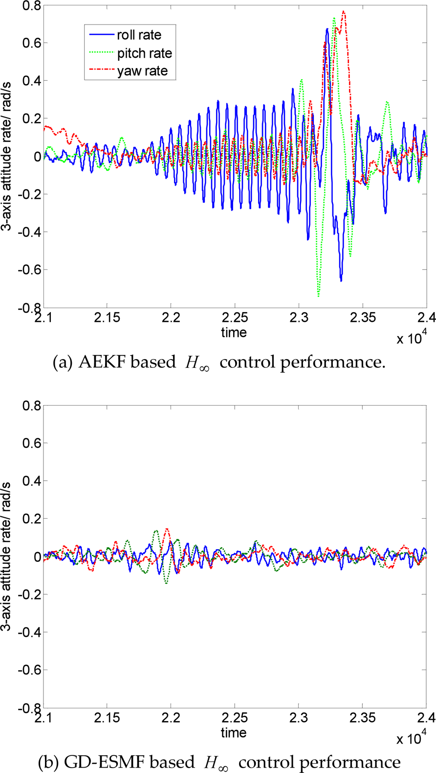
Tolerance control performance when actuator fault occurs

Figure 9.

AEKF and GD-ESMF AHC parameter estimation performance when actuator fault occurs

On the other hand, for the proposed GD-ESMF estimation method for actuator faults, the estimated boundaries were able to cover the true value of AHCs; therefore, the designed H_∞ controller was able to continuously keep the RUAV stable in hovering mode. This result shows that GD-ESMF for online fault modelling is more effective for actuator fault tolerance control when used in RUAVs, compared with the AEKF- based estimation method; thus, AEKF cannot be used under this flight mode.

The adaptive strategy of AEKF is the same with AUKF and only the precision of estimated mean value is lower than AUKF, due to linearization by the first order. The precision of estimated uncertainty boundaries is almost the same for AEKF and AUKF. Hence, compared with AEKF and AUKF, the above results were sufficient to verify that the AESMF has the best performance of computation efficiency and the best precision of estimated uncertainty boundaries for real applications, due to its adaptive strategy.

5. Conclusion

This paper proposed an AESMF application for actuator fault detection in RUAVs with uncertainty dynamics. AESMF's stability was firstly demonstrated mathematically and applied for on-line actuator failure modelling, based on AHCs. Compared with traditional ESMF, AUKF and AEKF, the results of flight experiments showed that the proposed scheme can automatically compensate for failures and effectively track the boundaries of fault parameters under UBB process noise, which is important for the fault model base control of RUAVs. The applicability of the proposed actuator fault detection algorithm was also verified in this flight test.

Footnotes

6.

This research was supported by The National Natural Science Foundation of China under Grant: 61203334 and 61433016.

References

Fengyou

and Shifan

(1996) A Highly Reliable Fault-Tolerant Microprocessor System for Industrial Process Control. Proceedings of IEEE International Conference on Industrial Technology, Tongji University, China: 355–357.

Zajac

(2014) Online fault detection of a mobile robot with a parallelized particle filter. Neurocomputing 126: 151–165.

Napolitano

and Seanor

(1998) Kalman Filters and Neural- Network Scheme for Sensor Validation in Flight Control Systems. IEEE Transaction on Control System Technology 6(5): 596–611.

Hao

Song

and Wang

(2013) Robust fault-tolerant control of uncertain fractional-order systems against actuator faults. IET Transactions on Control Theory & Applications 7(9): 193–202.

Zhang

and Jin

(2001) Integrated active fault-tolerant control using IMM approach. IEEE Transactions on Aerospace and Electronic Systems 37(4): 210–223.

Fradkov

and Andrievsky

(2005) Combined adaptive controller for UAV guidance. European Journal of Control 11(1): 71–79.

Eric

and Suresh

(2005) Adaptive Trajectory Control for Autonomous Helicopters. Journal of Guidance, Control, and Dynamics 28(3): 524–538.

Guillaume

and Hans

(2008) Efficient Nonlinear Actuator Fault Detection and Isolation System for Unmanned Aerial Vehicles. Journal of Guidance, Control, and Dynamics 31(1): 225–237.

Van

and Wan

(2001) The Square-root Unscented Kalman Filter for State and Parameter-estimation. Proceedings of the International Conference on Acoustics, Speech and Signal Processing, Salt Lake City, USA: 3461–3466.

10.

Heredia

and Ollero

(2011) Detection of Sensor Faults in Small Helicopter UAVs Using Observer/Kalman Filter Identification. Mathematical Problems in Engineering ID174618.

11.

Hathaway

and Gandhi

(2008) Tilt rotor Whirl Flutter Alleviation Using Actively Controlled Wing Flaperons. AIAA Journal 44 (11): 2524–2534.

12.

Yeo

and Johnson

(2005) Assessment of Comprehensive Analysis Calculation of Air loads on Helicopter Rotors. Journal of Aircraft 42 (5): 1218–1228.

13.

Gandhi

(2004) Helicopter Vibration Reduction Using Fixed-System Auxiliary Moments. AIAA Journal 42 (3): 501–512.

14.

Theodore

Tischler

and Colbourne

(2004) Rapid Frequency-Domain Modeling Methods for Unmanned Aerial Vehicle Flight Control Applications. Journal of Aircraft 41(4): 735–743.

15.

Metlter

Denver

and Feron

(2004) Scaling Effects and Dynamic Characteristics of Miniature Rotorcraft. Journal of Guidance, Control, and Dynamics 27 (3): 466–478.

16.

Haykin

and deFreitas

(2004) Special issue on sequential state estimation. Proceedings of the IEEE 93: 99–400.

17.

Ahrens

and Khalil

(2007) Closed-loop behavior of a class of nonlinear systems under EKF-based control. IEEE Transactions on Automatic Control 52: 536–540.

18.

Julier

and Uhlmann

(2004) Unscented filtering and nonlinear estimation. Proceedings of the IEEE 92: 401–422.

19.

Park

Lee

and Park

(2009) Correction Robot pose for SLAM based on Extended Kalman Filter in a Rough Surface Environment. International Journal of Advanced Robotic Systems 6: 67–72.

20.

Salvatore

Stasi

and Tarchioni

(1993) A new EKF-based algorithm for flux estimation in induction machines. IEEE Transactions on Industrial Electronics 40(5): 496–504.

21.

Julier

Uhlmann

and Durrant-Whyte

(2000) A new method for the nonlinear transformation of means and covariances in filters and estimators. IEEE Transactions on Automatic Control 45(3): 477–482.

22.

Rigatos

(2011) Derivative-Free Nonlinear Kalman Filtering for MIMO Dynamical Systems: Application to Multi-DOF Robotic Manipulators. International Journal of Advanced Robotic Systems 8: 47–61.

23.

Hadi

Chamseddine

and Zhang

(2013) Experimental Test of a Two-Stage Kalman Filter for Actuator Fault Detection and Diagnosis of an Unmanned Quadrotor Helicopter. Journal of Intelligent and Robotics Systems 70(1–4): 107–117.

24.

Zhang

Chamseddine

and Rabbath

(2013) Development of advanced FDD and FTC techniques with application to an unmanned quadrotor helicopter testbed. Journal of Franklin Institute – Engineering and Mathematics 350(9): 2396–2422.

25.

Jiang

Song

and Han

(2007) A novel adaptive unscented Kalman filter for nonlinear estimation. IEEE Conference on Decision and Control, New Orleans, USA: 4293–4298.

26.

Scholte

and Campbell

(2003) A nonlinear set-membership filter for on-line applications. International Journal of Robust and Nonlinear Control 13(15): 1337–1358.

27.

Zhou

Han

and Liu

(2007) A UD factorization-based nonlinear adaptive set-membership filter for ellipsoidal estimation. International Journal of Robust and Nonlinear Control 18(16): 513–1531.

28.

Song

Han

and Liu

(2013) Active Model-Based Predictive Control and Experimental Investigation on Unmanned Helicopters in Full Flight Envelope. IEEE Transactions on Control Systems Technology 21(4): 1502–1509.

29.

Song

and Han

(2012) A MIT-based nonlinear adaptive set- membership filter for ellipsoidal estimation of mobile robots' states. International Journal of Advanced Robotic Systems 9(131): 1–12.

30.

Shim

(2000) Hierarchical flight control system synthesis for rotorcraft-based unmanned aerial vehicles. Ph.D. Dissertation, Mechanical Engineering Department, University of California, Berkeley.

31.

Done

and Balmford

(2001) Bramwell's helicopter dynamics, 2nd edition, Butterworth Heinemann, UK.

32.

Bilal

and Hemanshu

(2011) Dynamic Compensation for Control of a Rotary wing UAV Using Positive Position Feedback. Journal of Intelligent & Robotic Systems 61(1–4): 43–56.

33.

Song

and Han

(2012) KF-based Adaptive UKF Algorithm and its application for Rotorcraft UAV Actuator Failure Estimation, International Journal of Advanced Robotic Systems 9(132): 1–9.

34.

Han

and Wu

(2008), Rotorcraft UAV Actuator Failure Estimation with KF-based Adaptive UKF Algorithm, American Control Conference, Washington, USA, June 11–13: 1618–1623.

35.

Song

Dai

Han

and Wang

(2010) The New Evolution for SIA Rotorcraft UAV Project. Journal of Robotics ID743010.

36.

Song

Dai

Han

and Liu

, Modeling a small-size unmanned helicopter using optimal estimation in the frequency domain. International Journal of Intelligent Systems Technologies and Applications, 2010, 8 (1–4): 70–85

37.

Wang

Song

and Han

(2013) A Full-functional Simulation and Test Platform for Rotorcraft Unmanned Aerial Vehicle Autonomous Control. Advances in Intelligent Systems and Computig 208: 537–547.

38.

Ho-Chan

Hardian

Taesam

Agus

Gigun

and Widyawardana

(2012) Parameter identification and design of a robust attitude controller using H ∞ methodology for the raptor E620 small-scale helicopter. International Journal of Control Automation and Systems 10(1): 88–101.

Experimental Investigation for RUAV's Actuator Fault Detections with AESMF

Abstract

Keywords

1. Introduction

2.1 RUAV Dynamics Modelling

3.1 AESMF Algorithm Review

4. Simulations and Flight Experiments

4.1 Flight Test Platform

Footnotes

6.

References