Sage Journals: Discover world-class research

Abstract

Based on screw theory, a novel improved inverse-kinematics approach for a type of six-DOF serial robot, “Qianjiang I”, is proposed in this paper. The common kinematics model of the robot is based on the Denavit-Hartenberg (D-H) notation method while its inverse kinematics has inefficient calculation and complicated solution, which cannot meet the demands of online real-time application. To solve this problem, this paper presents a new method to improve the efficiency of the inverse kinematics solution by introducing the screw theory. Unlike other methods, the proposed method only establishes two coordinates, namely the inertial coordinate and the tool coordinate; the screw motion of each link is carried out based on the inertial coordinate, ensuring definite geometric meaning. Furthermore, we adopt a new inverse kinematics algorithm, developing an improved sub-problem method along with Paden-Kahan sub-problems. This method has high efficiency and can be applied in real-time industrial operation. It is convenient to select the desired solutions directly from among multiple solutions by examining clear geometric meaning. Finally, the effectiveness and reliability performance of the new algorithm are analysed and verified in comparative experiments carried out on the six-DOF serial robot “Qianjiang I”.

Keywords

Inverse Kinematics Screw Theory Paden-Kahan Sub-problems Serial Robot

Symbol List

ω	angular velocity of rotation
v	linear velocity of translation
ξ	unit motion twist
$e^{\hat{ξ} θ}$	twist exponential form
$\hat{ω}$	skew symmetric matrix
q _i	intermediate point
g _i	configuration of rigid
u, v, z	variable
r _i	reference point
α, β, γ	coefficient

1. Introduction

The most popular method used in robot kinematics is based on the Denavit-Hartenberg (D-H) notation with the homogeneous transformation of points [1]. In this method, the kinematic formula of each joint is described by one coordinate system in relation to another, resulting in some singularity problems. The inverse kinematics based on the D-H method has inefficient calculation and complicated solution, which will make real-time online operation less effective; this may not be suitable for real-time circumstances. As a traditional algorithm, the D-H-based inverse transformation method [1] is widely used for its intuition, but the inverse of each 4×4 homogeneous transformation matrix needs to be worked out, which results in a complex and time-consuming solution process. Thus, the effectiveness of the inverse-kinematics solution process directly affects the results of real-time online motion control [2, 3], for example as in the inverse dynamics controller in [4] and the remote robot operation in [5].

In recent years, another method based on screw theory has been increasingly adopted in kinematics modelling both for serial robots and parallel robots [6–8]. A screw motion is represented as a linear motion along an axis with a rotation motion by an angle about the same axis in relation to the inertial frame [6]. In screw theory every transformation of rigid body with respect to the inertial coordinate system can be expressed by a screw displacement [9].

In [10] a comparative analysis between the screw theory method and the D-H method for kinematics is presented, which shows that the screw-based method has some striking advantages over the D-H method. There are two main advantages of using the screw method to describe rigid body kinematics. The first is that it allows a global description of rigid body motion that does not suffer from singularity problems without using local coordinates. It needs only two coordinates, of which one is the inertial frame at the base and the other the tool frame at the end-effectors. All joint motions are described in the base coordinate. The second advantage of the method is that it can greatly simplify the analysis of mechanisms by using a geometric description of rigid motion and easily define the geometrical significance of the inverse kinematics solutions. Hence, it is easy to implement the movement of the robot knowing each joint's obvious geometric meaning [11].

Besides the merits mentioned above, the screw theory method also can avoid a large amount of matrixes multiplying operation, which can result in fast calculation and compact formalizations compared to D-H notation method [12]. In [13], Wu's method is introduced to the process of inverse kinematics by combining the idea of characteristic set with the screw method. In [14], screw theory is implemented to analyse the limitations and provides geometric interpretation of the sensible wrenches of continuum robots. With screw theory to solve the inverse kinematics problem we generally reduce the full inverse kinematics problem of a serial robot into some appropriate sub-problems whose solutions are already known. For a robot only including rotary joints, three basic Paden-Kahan sub-problems [15] based on screw theory are admissible for some configurations of robot inverse kinematics. In [16] an extended solution of sub-problem 2 is developed to respond to more manipulator configurations. However, the existing methods of Paden-Kahan sub-problems cannot solve all configurations of robot inverse kinematics. Taking a particular configuration of the six-DOF serial robot “Qianjiang I” as an example, it is not suitable to apply the known Paden-Kahan sub-problems to solve the full inverse kinematic problem. Hence, in this paper a novel improved Paden-Kahan sub-problem is studied for this particular configuration of six-DOF serial robot; then, the new inverse kinematic algorithm is proposed to simplify the solution process and promote efficiency with the virtues of the screw theory.

In section II we provide the necessary notation of the kinematic description of rigid body based on the screw theory and introduce some basic Paden-Kahan sub-problems. Section III presents a novel sub-problem solution with a special configuration of the series revolute joints. In section IV we implement the full inverse kinematic algorithm for the special six-DOF “Qianjiang-I” by combining our proposed new sub-problem and other basic Paden-Kahan sub-problems. In section V a numerical example and comparative experiment are illustrated to verify the correctness and effectiveness of this proposed method. Section VI concludes this paper.

2. Screw theory of rigid body

A twist, ξ, represents the instantaneous motion of a rigid body relative to a referential axis in [15]. It is usually expressed as ξ = (ω^T; v^T)^T ∊ R⁶ where ω is the angular velocity of rotation about a certain axis and v is the instantaneously linear velocity of translation along the same axis, as shown in Figure 1.

Figure 1.

Screw motion

We consider g_st(0) as the initial configuration of the body coordinate system {B} relative to the inertial coordinate {A} at the base. After the twist motion ξ of the rigid body, the final configuration of {B} to {A} in twist exponential form is

g_{a b} = g_{s t} (θ) = e^{\hat{ξ} θ} g_{s t} (0)

(1)

where

\hat{ξ} = [\begin{matrix} \hat{ω} & v \\ 0 & 0 \end{matrix}]

e^{\hat{ξ} θ} = {\begin{matrix} [\begin{matrix} e^{\hat{ω} θ} & (I - e^{\hat{ω} θ}) (ω \times v) + θ ω ω^{T} v \\ 0 & 1 \end{matrix}], ω \neq 0 \\ [\begin{matrix} I & θ v \\ 0 & 1 \end{matrix}], ω = 0 \end{matrix}

e^{\hat{ω} θ} = I + \hat{ω} \sin θ + {\hat{ω}}^{^{2}} (1-cos θ)

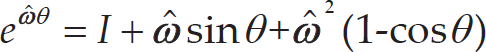
can correspond to ω=[ω₁ ω₂ ω₃]^T.

For a revolute joint:

ξ_{i} = [\begin{matrix} ω_{i} \\ r_{i} \times ω_{i} \end{matrix}]

(2)

For an open-chain serial robot with n revolute joints, the forward kinematics can be achieved by the product of the exponential formula in Eq.(1) as

g_{s t} (θ) = e^{{\hat{ξ}}_{1} θ_{1}} e^{{\hat{ξ}}_{2} θ_{2}} \dots e^{{\hat{ξ}}_{n} θ_{n}} g_{s t} (0)

(3)

As for the inverse kinematics problem, we can develop a geometrically effective algorithm by using the known inverse kinematics sub-problems. There are some basic Paden-Kahan sub-problems [15], as follows:

Rotation about a single axis.

Rotation about two subsequent axes.

Rotation to a given distance.

Though the basic Paden-Kahan sub-problems are applied widely in some configurations of robot, this is still not enough to respond to the general configuration structure. This paper therefore extends a novel sub-problem to solve some special configuration structures in series robots.

3. New sub-problem solution

The new sub-problem can be illustrated as in Figure 2, where there is rotation about three non-intersecting axis; two of these are parallel and non co-planar to the third.

The point q_a rotates θ₃ along ξ₃ axis to point q_b, then rotates θ₂ along ξ₂ axis to point q_c, and finally rotates θ₁ along ξ₁ axis to point q. Now we solve θ₁, θ₂ and θ₃ with the given q_a and q.

The twists’ motion can be represented as

e^{{\hat{ξ}}_{3} θ_{3}} q_{a} = q_{b}, e^{{\hat{ξ}}_{2} θ_{2}} q_{b} = q_{c}, e^{{\hat{ξ}}_{1} θ_{1}} q_{c} = q

e^{{\hat{ξ}}_{1} θ_{1}} e^{{\hat{ξ}}_{2} θ_{2}} e^{{\hat{ξ}}_{3} θ_{3}} q_{a} = q = [\begin{matrix} q_{x} \\ q_{y} \\ q_{z} \end{matrix}]

(4)

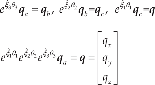
where ξ₁, ξ₂ and ξ₃ are unit magnitude twists with zero-pitch, non-intersecting axis with ξ₂, ξ₃ two parallel axis.

Figure 2.

New sub-problem structure

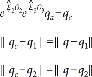
Applying the principle that the distance between points is preserved by rigid motion:

\begin{matrix} ‖ e^{{\hat{ξ}}_{1} θ_{1}} (e^{{\hat{ξ}}_{2} θ_{2}} e^{{\hat{ξ}}_{3} θ_{3}} q_{a} - q_{1}) ‖ = ‖ e^{{\hat{ξ}}_{2} θ_{2}} e^{{\hat{ξ}}_{3} θ_{3}} q_{a} - q_{1} ‖ \\ ‖ e^{{\hat{ξ}}_{1} θ_{1}} e^{{\hat{ξ}}_{2} θ_{2}} e^{{\hat{ξ}}_{3} θ_{3}} q_{a} - q_{1} ‖ = ‖ e^{{\hat{ξ}}_{2} θ_{2}} e^{{\hat{ξ}}_{3} θ_{3}} q_{a} - q_{1} ‖ = ‖ q - q_{1} ‖ \\ ‖ e^{{\hat{ξ}}_{1} θ_{1}} e^{{\hat{ξ}}_{2} θ_{2}} e^{{\hat{ξ}}_{3} θ_{3}} q_{a} - q_{2} ‖ = ‖ e^{{\hat{ξ}}_{2} θ_{2}} e^{{\hat{ξ}}_{3} θ_{3}} q_{a} - q_{2} ‖ = ‖ q - q_{2} ‖ \end{matrix}

(5)

where q₁ and q₂ are arbitrary different points on the axis ξ₁; here we choose the simplest:

q_{1} = [\begin{matrix} 0 \\ 0 \\ 0 \end{matrix}] q_{2} = [\begin{matrix} 0 \\ 0 \\ 1 \end{matrix}] ω_{2} = [\begin{matrix} 1 \\ 0 \\ 0 \end{matrix}]

(6)

From Eq.(4) and Eq.(5) we can get

\begin{matrix} e^{{\hat{ξ}}_{2} θ_{2}} e^{{\hat{ξ}}_{3} θ_{3}} q_{a} = q_{c} \\ ‖ q_{c} - q_{1} ‖ = ‖ q - q_{1} ‖ \\ ‖ q_{c} - q_{2} ‖ = ‖ q - q_{2} ‖ \end{matrix}

(q_{c} - q_{a}) \cdot ω_{2} = 0

(7)

Substituting Eq.(6) into Eq.(7) gives

q_{c} = [\begin{matrix} 0 \\ \pm \sqrt{q_{x}^{2} + q_{y}^{2}} \\ q_{z} \end{matrix}]

(8)

From Eq.(4) we have

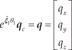
e^{{\hat{ξ}}_{1} θ_{1}} q_{c} = q = [\begin{matrix} q_{x} \\ q_{y} \\ q_{z} \end{matrix}]

(9)

Then, θ₁ can be obtained by applying the Paden-Kahan sub-problem 1 in [15]:

θ_{1} = a \tan 2 (- \pm \sqrt{q_{x}^{2} + q_{y}^{2}} q_{x}, \pm \sqrt{q_{x}^{2} + q_{y}^{2}} q_{y})

(10)

As for θ₂ and θ₃, we project the screw motion onto a plane which is perpendicular to axis ξ₂, ξ₃, as shown in Figure 3.

Figure 3.

(a) Two-parallel-screw motion. (b) Screw motion plane projection.

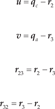
The vectors are set as

\begin{matrix} u = q_{c} - r_{2} \\ v = q_{a} - r_{3} \\ r_{23} = r_{2} - r_{3} \end{matrix}

r_{32} = r_{3} - r_{2}

(11)

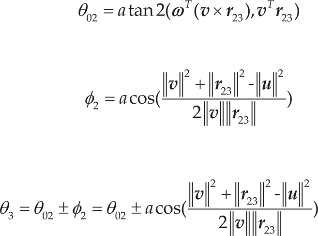
Using triangular geometry, we can find θ₀₁ and φ₁ as follows:

θ_{01} = a \tan 2 (ω^{T} (u \times r_{32}), u^{T} r_{32})

{‖ u ‖}^{2} + {‖ r_{23} ‖}^{2} - 2 ‖ u ‖ ‖ r_{23} ‖ \cos ϕ_{1} = {‖ v ‖}^{2}

(12)

is given by

θ_{2} = ϕ_{1} \pm θ_{01} = a \cos (\frac{{‖ u ‖}^{2} + {‖ r_{23} ‖}^{2} - {‖ v ‖}^{2}}{2 ‖ u ‖ ‖ r_{23} ‖}) \pm θ_{01}

(13)

Using the same method, we can find θ₃ as follows:

\begin{matrix} θ_{02} = a \tan 2 (ω^{T} (v \times r_{23}), v^{T} r_{23}) \\ ϕ_{2} = a \cos (\frac{{‖ v ‖}^{2} + {‖ r_{23} ‖}^{2} - {‖ u ‖}^{2}}{2 ‖ v ‖ ‖ r_{23} ‖}) \\ θ_{3} = θ_{02} \pm ϕ_{2} = θ_{02} \pm a \cos (\frac{{‖ v ‖}^{2} + {‖ r_{23} ‖}^{2} - {‖ u ‖}^{2}}{2 ‖ v ‖ ‖ r_{23} ‖}) \end{matrix}

(14)

The results above indicate that this sub-problem may have one solution, multiple solutions or no solution, depending on whether the rotational surfaces of axis ξ₂, ξ₃ intersect or not. When the two circles have two intersections, as in Figure 3(b), there are two solutions for the sub-problem. When the two circles are tangential to each other, there exists only one solution. There will be no solution where the two circles are not intersecting.

4. Inverse kinematics of six-DOF series robot

4.1 Kinematic modelling

The six-DOF industrial welding serial Robot “Qianjiang I” has six revolute joints and the structure coordinates are shown as Figure 4.

As illustrated in the figure, the last three consecutive joints’ axes intersect at a point while the first three joints’ structure satisfies the new sub-problem situation presented in Section 3. To solve the inverse kinematics problem of the whole robot, we can reduce it into some appropriate sub-problems whose solutions are already known. We can apply the new sub-problem for the inverse kinematics of the first three joints and apply the Paden-Kahan sub-problems to the inverse kinematics of the last three consecutive joints.

Figure 4.

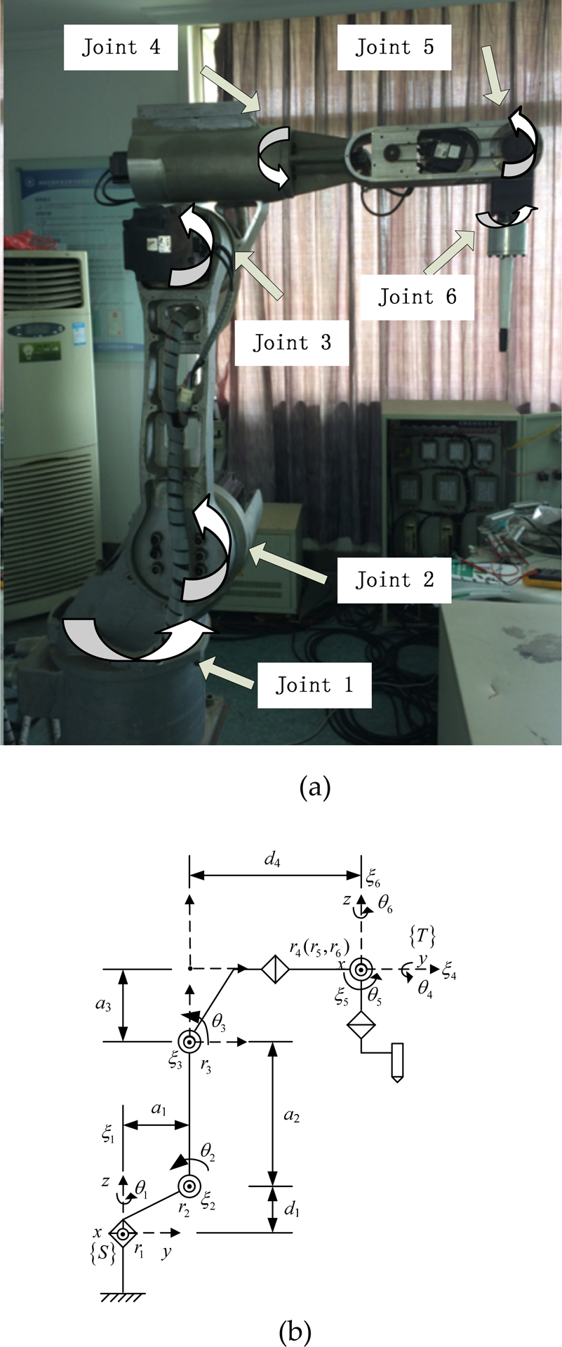
(a) “Qianjiang I”. (b) Structure coordinates.

Firstly, we construct the twist of each joint:

\begin{matrix} ω_{1} = [\begin{matrix} 0 \\ 0 \\ 1 \end{matrix}] ω_{2} = [\begin{matrix} 1 \\ 0 \\ 0 \end{matrix}] ω_{3} = [\begin{matrix} 1 \\ 0 \\ 0 \end{matrix}] ω_{4} = [\begin{matrix} 0 \\ 1 \\ 0 \end{matrix}] ω_{5} = [\begin{matrix} 1 \\ 0 \\ 0 \end{matrix}] ω_{6} = [\begin{matrix} 0 \\ 0 \\ 1 \end{matrix}] \\ r_{1} = [\begin{matrix} 0 \\ 0 \\ 0 \end{matrix}] r_{2} = [\begin{matrix} 0 \\ a_{1} \\ d_{1} \end{matrix}] r_{3} = [\begin{matrix} 0 \\ a_{1} \\ d_{1} + a_{2} \end{matrix}] r_{4} = r_{5} = r_{6} = [\begin{matrix} 0 \\ a_{1} + d_{4} \\ d_{1} + a_{2} + a_{3} \end{matrix}] \\ ξ_{1} = [\begin{matrix} 0 \\ 0 \\ 1 \\ 0 \\ 0 \\ 0 \end{matrix}] ξ_{2} = [\begin{matrix} 1 \\ 0 \\ 0 \\ 0 \\ d_{1} \\ - a_{1} \end{matrix}] ξ_{3} = [\begin{matrix} 1 \\ 0 \\ 0 \\ 0 \\ a_{2} + d_{1} \\ - a_{1} \end{matrix}] \\ ξ_{4} = [\begin{matrix} 0 \\ 1 \\ 0 \\ - a_{2} - d_{1} - a_{3} \\ 0 \\ 0 \end{matrix}] ξ_{5} = [\begin{matrix} 1 \\ 0 \\ 0 \\ a_{1} + d_{4} \\ 0 \\ 0 \end{matrix}] ξ_{6} = [\begin{matrix} 0 \\ 0 \\ 1 \\ 0 \\ a_{2} + a_{3} + d_{1} \\ - a_{1} - d_{4} \end{matrix}] \end{matrix}

(15)

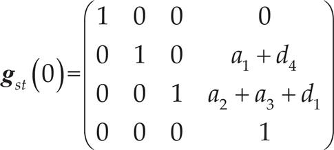
The initial configuration of Figure 4(b) is

g_{s t} (0) = (\begin{matrix} 1 & 0 & 0 & 0 \\ 0 & 1 & 0 & a_{1} + d_{4} \\ 0 & 0 & 1 & a_{2} + a_{3} + d_{1} \\ 0 & 0 & 0 & 1 \end{matrix})

(16)

Then, the forward kinematics of the six-DOF industrial welding robot is

g_{s t} (θ) = e^{{\hat{ξ}}_{1} θ_{1}} e^{{\hat{ξ}}_{2} θ_{2}} \dots e^{{\hat{ξ}}_{6} θ_{6}} g_{s t} (0) = (\begin{matrix} n_{x} & o_{x} & a_{x} & p_{x} \\ n_{y} & o_{y} & a_{y} & p_{y} \\ n_{z} & o_{z} & a_{z} & p_{z} \\ 0 & 0 & 0 & 1 \end{matrix})

(17)

4.2 Solving for the inverse kinematics

Step 1 Solving θ₁, θ₂, θ₃

When given the pose position and orientation of end-effectors in Eq.(17), we can solve the first three joints, θ₁, θ₂, θ₃, by applying the proposed sub-problem in Section 3. In this case, we can set the known parameters as follows:

q = [\begin{matrix} q_{x} \\ q_{y} \\ q_{z} \end{matrix}] and q_{a} = [\begin{matrix} 0 \\ a_{1} + d_{4} \\ d_{1} + a_{2} + a_{3} \end{matrix}]

(18)

Finally, we substitute these parameters into Eq.(4), and solve θ₁, θ₂, θ₃ accordingly.

Step 2 Solving θ₄ and θ₅

From Eq.(17) and the known θ₁, θ₂, θ₃, we have

e^{{\hat{ξ}}_{4} θ_{4}} e^{{\hat{ξ}}_{5} θ_{5}} e^{{\hat{ξ}}_{6} θ_{6}} = e^{- {\hat{ξ}}_{3} θ_{3}} e^{- {\hat{ξ}}_{2} θ_{2}} e^{- {\hat{ξ}}_{1} θ_{1}} g_{s t} (θ) = g_{1}

(19)

The simple point q₆ is chosen on the ξ₆ axis, but not on the axis of ξ₄, ξ₅ as

q_{6} = [\begin{matrix} 0 \\ a_{1} + d_{4} \\ 0 \end{matrix}]

(20)

Then, the q₆ on both sides of Eq.(19) is multiplied, giving

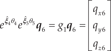
e^{{\hat{ξ}}_{4} θ_{4}} e^{{\hat{ξ}}_{5} θ_{5}} q_{6} = g_{1} q_{6} = [\begin{matrix} q_{x 6} \\ q_{y 6} \\ q_{z 6} \end{matrix}]

(21)

Thus, we can solve this case directly by applying the Paden-Kahan sub-problem 2 in [15], from which we have:

\begin{matrix} α = \frac{(ω_{4}^{T} ω_{5})(ω_{5}^{T} u)- ω_{4}^{T} v}{{(ω_{4}^{T} ω_{5})}^{5} - 1} = q_{y 6} - a_{1} - d_{4} \\ β = \frac{(ω_{4}^{T} ω_{5})(ω_{5}^{T} v)- ω_{5}^{T} u}{{(ω_{4}^{T} ω_{5})}^{5} - 1} = 0 \\ γ = \pm \sqrt{\frac{∥ u ∥^{2} - α^{2} - β^{2} - 2 α β (ω_{4}^{T} ω_{5})}{∥ ω_{4}^{} \times ω_{5} ∥}} \\ = \pm \sqrt{{(d_{1} + a_{2} + a_{3})}^{2} - {(q_{y 6} - a_{1} - d_{4})}^{2}} \\ z = α ω_{4} + β ω_{5} + γ (ω_{4} \times ω_{5}) = [\begin{matrix} 0 \\ α \\ - γ \end{matrix}] \\ c = z + q_{w} = [\begin{matrix} 0 \\ q_{y 6} \\ - γ + d_{1} + a_{2} + a_{3} \end{matrix}] \end{matrix}

(22)

Finally, this yields:

\begin{matrix} e^{{\hat{ξ}}_{5} θ_{5}} q_{6} = c \\ e^{{\hat{ξ}}_{4} θ_{4}} c = q \end{matrix}

(23)

Then, in this case we employ the Paden-Kahan sub-problem 1 in [15], giving

\begin{array}{l} θ_{5} = a \tan 2 (ω^{T} (u^{'} \times v^{'}), {u^{'}}^{T} v^{'}) = a \tan 2 ((q_{y 6} - a_{1} - d_{4}), γ) \\ θ_{4} = a \tan 2 (ω^{T} (u^{'} \times v^{'}), {u^{'}}^{T} v^{'}) \\ = a \tan 2 (- γ q_{x 6}, {(q_{y 6} - a_{1} - d_{4})}^{2} + γ (d_{1} + a_{2} + a_{3} - q_{z 6})) \end{array}

(24)

Eq. (24) has two solutions corresponding to the results of γ in Eq. (22).

Step 3 Solving θ₆

From Eq.(19), we get

e^{{\hat{ξ}}_{6} θ_{6}} = e^{- {\hat{ξ}}_{5} θ_{5}} e^{- {\hat{ξ}}_{4} θ_{4}} e^{- {\hat{ξ}}_{3} θ_{3}} e^{- {\hat{ξ}}_{2} θ_{2}} e^{- {\hat{ξ}}_{1} θ_{1}} g_{s t} (θ) = g_{2}

(25)

The reference point q_t is chosen, though not on the ξ₆ axis, as

q_{t} = [\begin{matrix} 0 \\ a_{1}^{} \\ d_{1} + a_{2} + a_{3} \end{matrix}]

(26)

Then, the q_t is multiplied on both sides of Eq.(25), giving

e^{{\hat{ξ}}_{6} θ_{6}} q_{t} = g_{2} q_{t} = [\begin{matrix} q_{t x 6} \\ q_{t y 6} \\ q_{t z 6} \end{matrix}]

(27)

Then, in this case we employ the Paden-Kahan sub-problem 1 in [15], giving

\begin{array}{l} θ_{6} = a \tan 2 (ω^{T} (u^{'} \times v^{'}), {u^{'}}^{T} v^{'}) \\ = a \tan 2 (d_{4} q_{t x}, - d_{4} (q_{t y} - a_{1} - d_{4})) \end{array}

(28)

In sum, the full inverse-kinematic closed solutions are solved by applying the new sub-problem and basic Paden-Kahan problems. In the process of solving, we can choose the most suitable and simple reference points, such as (6), (20) and (26), resulting in a simplification of the calculating process and an improvement of the computation efficiency. Additionally, the obvious geometric meaning allows us to select the desired and reasonable solutions easily.

5. Example and experiment

To verify the correctness of the inverse kinematics algorithm, we choose an arbitrary group of joint angles within the bounds of workspace range (−π, π]:

θ_{1} = \frac{π}{4}, θ_{2} = 0, θ_{3} = \frac{π}{2}, θ_{4} = π, θ_{5} = \frac{π}{4}, θ_{6} = - \frac{π}{8}

(29)

with the structure parameters

\begin{array}{l} d_{1} = 250 m m, a_{1} = 150 m m, a_{2} = 550 m m, \\ a_{3} = 160 m m, d_{4} = 594 m m \end{array}

(30)

Applying the forward kinematics gives the pose position and orientation of the end-effectors:

g_{s t} (θ) = [\begin{matrix} - 0.46196 & - 0.73254 & - 0.50000 & 7.07100 \\ - 0.84464 & 0.19134 & 0.50000 & - 7.07100 \\ - 0.27060 & 0.65330 & - 0.70710 & 1400 \\ 0 & 0 & 0 & 1 \end{matrix}]

(31)

Then, taking Eq.(31) as a known condition, we solve the inverse kinematics by applying the new sub-problem and the basic Paden-Kahan sub-problems. The solutions are shown in Table 1, and the configuration simulation model of each solution are shown in Figure 5.

Table 1.

Eight solutions of the inverse kinematics

No.	Joint	θ[°]	Joint	θ[°]
1	1	45.00000001	4	180.00000000
	2	0.00000012	5	44.99999145
	3	90.00000002	6	−22.49999885
2	1	45.00000001	4	0
	2	0.00000012	5	135.00000855
	3	90.00000002	6	157.50000115
3	1	45.00000001	4	180.00000000
	2	15.84111248	5	30.97777657
	3	60.13711126	6	−22.49999694
4	1	45.00000001	4	0
	2	15.84111248	5	149.02222343
	3	60.13711126	6	157.50000306
5	1	−134.99999998	4	0
	2	−1.95792331	5	45.11668894
	3	91.84000059	6	−22.49699928
6	1	−134.99999998	4	180.00000000
	2	−1.95792331	5	134.88331106
	3	91.84000059	6	157.50300072
7	1	−134.99999998	4	0
	2	15.83992123	5	60.86405665
	3	58.2963389	6	−22.496155618
8	1	−134.99999998	4	180.00000000
	2	15.83992123	5	119.13594335
	3	58.2963389	6	157.50384438

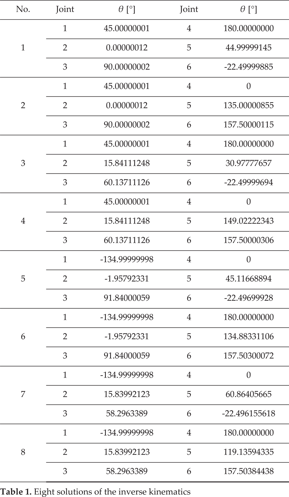
From the result above, there are eight solutions of the inverse kinematics, and the first solution is perfect with the given joint in Eq.(29), which verifies the correctness and high accuracy of the presented inverse kinematics algorithm. Furthermore, in real mechanisms when considering the caging device and the actual workspace of the robot, a series of position bounds for every joint need be set. This additional geometrical information may help select the desired and reasonable solution during the inverse kinematic computing process using the proposed method. In real robot operation, we should also adopt optimization strategies such as the minimum energy method or minimum joint-displacement method, and choose a suitable solution for robot control without collision.

Figure 5.

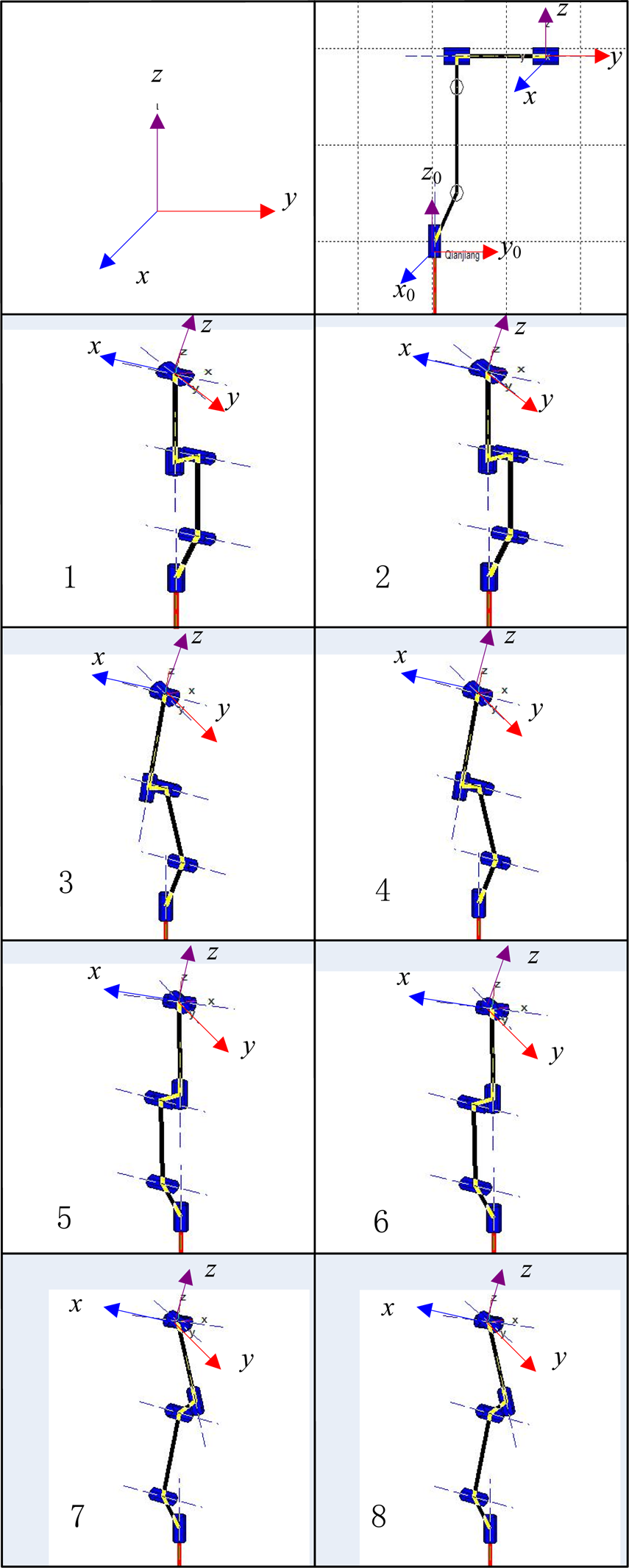
Configuration simulation models

To verify the efficiency and reliability performance in real control of the proposed algorithm, we choose a closed-curve irregular trajectory to track in Figure 6(a). Before applying the inverse kinematic algorithm, we sampled 681 discrete points from the curve in Figure 6(b) and calculated the Cartesian coordinate of each point as the desired pose matrix of the end-effector. The inverse kinematics of these poses needed be solved for the next step of trajectory planning in joint space.

Figure 6.

(a) Closed-curve irregular trajectory. (b) Sampled discrete points.

To show the correctness and efficiency of our proposed method, we compare our screw theory method (“STM”) in this paper with the traditional inverse transformation method (“TIT”) in [17] and the vector-dot-product method (“VDP”) in [18]. Then, we implement these different algorithms to solve the inverse kinematics of the closed-curve irregular trajectory in Figure 6, respectively, in VC++ software (Windows XP 32-bit, Intel Core i5, 2.57GHz CPU, 4GB DDR3), and record the computation time of each given pose matrix respectively 1000 times. The performance comparison results are shown in Table 2.

Table 2.

Performance comparisons of different algorithms

	Mean time (us)	Max time (us)
TIT	11.683	12.579
VDP	6.457	8.191
STM	4.151	4.913

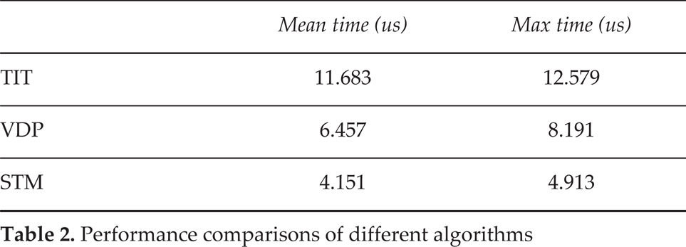
As shown in Table 2, our proposed STM method with the geometric characteristic is more effective in determining kinematics solutions than the other two methods. To be more specific, it only requires just under 4.151 μs to figure out the inverse kinematics solutions for one sample pose based on mean time with our STM. Comparatively, the TTM and VDP take almost 11.683 μs and 6.457 μs, respectively, due to their complicated matrix computation. The max time results show the performance of our proposed algorithm is better than others.

6. Conclusion

Concentrating on simplifying the calculation of inverse kinematics problems for serial robots, this paper has presented a new sub-problem solution, which extends the application of sub-problem solutions in the inverse kinematics of general configuration robots. The proposed method can avoid complex matrix inverse operation and make the choice among multiple solutions easier and faster due to the obvious geometric meaning. Further, the case of the six-DOF “Qianjiang I” inverse kinematics problem has been studied by reducing the full inverse kinematics into some sub-problems, namely, our novel sub-problem and the other Paden-Kahan sub-problems, which makes the formula calculation simple and the geometric meaning clear. The results verify the correctness and completeness of the novel screw-theory-based inverse kinematics algorithm. Finally, the efficiency and reliability performance of our method (STM) has been compared in a closed-curve irregular trajectory tracking experiment with other two inverse kinematics algorithms, revealing that the STM algorithm is more practical and can meet the high-performance requirements of real-time operation. In future work, the inverse algorithm for other general structural six-DOF serial robots can be studied based on the approach presented in this paper.

Footnotes

7.

The authors express sincere thanks to the editors, reviewers and all the members of our research group for their beneficial comments. The research work is jointly supported by the Science Fund for Creative Research Groups of the National Natural Science Foundation of China (No. 51221004) and Zhejiang Provincial Natural Science Foundation of China (No. LY13E050001), and Hangzhou Civic Significant Technological Innovation Project of China (No. 20132111A04).

References

Spong

Hutchinson

Vidyasagar

(2006) Robot modelling and control. New York: John Wiley & Sons.

Kucuk

Bingul

(2004) The inverse kinematics solutions of industrial robot manipulators. International Conference on Mechatronics, 3–5 June, Tunis, Tunisia, IEEE: 274–279.

Kucuk

Bingul

(2006) Robot kinematics: forward and inverse kinematics. Industrial Robotics Theory Modelling & Control. Germany: 117–148.

Matsuda

Tsukamoto

Matsumoto

(2014) Remote Operation System of Robot Arm with Visual Servo Mechanism by Target Selection. International Journal of Innovative Computing, Information & Control. 10 (4): 1381–1390.

Chen

Mei

(2014) Robust Adaptive Inverse Dynamics Control for Uncertain Robot Manipulator. International Journal of Innovative Computing, Information & Control. 10 (2): 575–587.

Crane

Rico

Duffy

(2006) Screw theory and its application to spatial robot manipulators. London: Cambridge University Press.

Sariyildiz

Temeltas

(2009) Solution of inverse kinematic problem for serial robot using quaterninons. International Conference on Mechatronics and Automation (ICMA), 9–12 Aug, Changchun, China, IEEE: 26–31.

Frisoli

Solazzi

Pellegrinetti

(2011) A new screw theory method for the estimation of position accuracy in spatial parallel manipulators with revolute joint clearances. Mechanism and Machine Theory. 46: 1929–1949.

Gallardo-Alvarado

Aguilar-Nájera

C.R

Casique-Rosas

(2008) Kinematics and dynamics of 2 (3-RPS) manipulators by means of screw theory and the principle of virtual work. Mechanism and Machine Theory. 43(10): 1281–1294.

10.

Sariyildiz

Cakiray

Temeltas

(2011) A comparative study of three inverse kinematic methods of serial industrial robot manipulators in the screw theory framework. International Journal of Advanced Robotic Systems. 8: 9–24.

11.

Rocha

Tonetto

Dias

(2011) A comparison between the Denavit–Hartenberg and the screw-based methods used in kinematic modelling of robot manipulators. Robotics and Computer-Integrated Manufacturing. 27(4): 723–728.

12.

Selig

(2000) Geometrical foundations of robotics. NJ, USA: World Scientific Publishing Co., Inc.

13.

S.Z.

Zhang

D.W.

Liu

H.N.

(2010) Solution of screw equation for inverse kinematics of 6R robot based on Wu's method. Journal of Mechanical Engineering. 46(17): 35–41.

14.

Simaan

(2008) An investigation of the intrinsic force sensing capabilities of continuum robots. IEEE Transactions on Robotics. 24(3): 576–587.

15.

Murray

R.M

Sastry

S.S.

(1994) A mathematical introduction to robotic manipulation. Boca Raton, FL: CRC Press.

16.

Tan

Y.S

Xiao

A.P.

(2008) Extension of the second paden-kahan sub-problem and its application in the inverse kinematics of a manipulator. International Conference on Robotics, Automation and Mechatronics. 21–24 Sept, Chengdu, China, IEEE: 379–381.

17.

Lenarcic

Husty

(2012) Latest Advances in Robot Kinematics. Springer Netherlands.

18.

Liu

H.S

Zhu

S.Q

J.B

(2008) Real-time inverse kinematics algorithm based on vector dot product. Transactions of the Chinese Society for Agricultural Machinery. 6: 212–216.