Inverse Kinematic Analysis of a Redundant Hybrid Climbing Robot

Abstract

This paper presents the complete inverse kinematic analysis of a novel redundant truss-climbing robot with 10 degrees of freedom. The robot is bipedal and has a hybrid serial-parallel architecture, where each leg consists of two parallel mechanisms connected in series. By separating the equation for inverse kinematics into two parts - with each part associated with a different leg - an analytic solution to the inverse kinematics is derived. In the obtained solution, all the joint coordinates are calculated in terms of four or five decision variables (depending on the desired orientation) whose values can be freely decided due to the redundancy of the robot. Next, the constrained inverse kinematic problem is also solved, which consists of finding the values of the decision variables that yield a desired position and orientation satisfying the joint limits. Taking the joint limits into consideration, it is shown that all the feasible solutions that yield a given desired position and orientation can be represented as 2D and 3D sets in the space of the decision variables. These sets provide a compact and complete solution to the inverse kinematics, with applications for motion planning.

1. Introduction

During the last two decades, there has been increasing interest in using climbing robots to perform dangerous tasks on vertical structures. Working on tall structures is very dangerous for human operators, who are exposed to the risk of falling from height, among others. Examples of such tasks include the periodic cleaning and inspection of glass façades in tall buildings [1], the periodic inspection and maintenance of metallic bridges [2] and power transmission lines [3], the inspection of welded unions in the construction industry [4], and tree climbing for branch trimming or fumigation [5]. Other applications of climbing robots can be found in [6], which also presents a comprehensive review of their main locomotion methods and adhesion technologies.

Truss structures are a particular type of vertical structure present in constructions such as metallic bridges, airports, telecommunications towers and power transmission lines. To achieve the high degree of mobility needed to explore these structures, truss-climbing robots typically have two grippers connected through a kinematic chain with some degrees of freedom (DOF). The locomotion method of these robots consists of grasping the structure with one of the grippers and using the kinematic chain to place the other gripper in the following attachment point of the structure. Next, the free gripper is fixed to the structure, acting as the new supporting point, and the previously fixed gripper is released, becoming the free gripper. This cycle is repeated again, and the robot advances through the structure swapping the roles of the fixed and free grippers.

Truss-climbing robots can be classified into three types [7]: serial, parallel and hybrid. Serial climbing robots have larger workspaces than parallel ones, but they are less rigid and have a limited payload. For example, [4] and [7] present serial climbing robots with six and four DOF, respectively. Other serial architectures inspired by inch worms, with five and eight DOF, are presented in [8, 9]. Other authors propose inchworm-like robots driven by flexible actuators which can climb poles [10] or travel inside pipelines [11]. A modular climbing robot is presented in [12], whose number of DOF can be modified by adding new modules. Finally, [13] presents three-DOF robots that can individually explore trusses or can be combined with other robots to form more complex robots with higher manoeuvrability.

Parallel climbing robots have a higher payload-to-weight ratio than serial robots but their workspace is more limited. A Gough-Stewart platform for climbing truss structures, pipelines and palm trees is proposed in [5].

Finally, hybrid climbing robots are composed of some serially connected parallel mechanisms. Reference [14] presents a hybrid climbing robot that combines a 3-RPR parallel mechanism with a rotation module connected in series. Another 12-DOF hybrid robot is proposed in [15]. In this case, the robot is bipedal and each leg is the serial combination of two 3-RPS parallel robots.

As these examples show, many truss-climbing robots have been proposed, mainly with a serial architecture. Nevertheless, the features of hybrid architectures make them specially interesting for climbing truss structures. On the one hand, hybrid robots have the high manoeuvrability and large workspace of serial robots, which is beneficial for exploring complex 3D structures. On the other hand, they also have the high rigidity and load-to-weight ratio of parallel robots, which is useful for climbing robots since they must support their own weight [16].

Considering these benefits of hybrid architectures, a new truss-climbing hybrid robot has been designed. The robot, shown in Figure 1, has two legs which are composed of two parallel mechanisms connected in series. The design of its legs permits the robot to easily execute the movements necessary to explore 3D trusses, such as convex and concave transitions between different planes, transitions between beams with different orientations, and the negotiation of obstacles. The robot has 10 DOF between the feet (grippers), which makes it redundant.

This paper is focused on the inverse kinematic analysis of this robot, which is a prerequisite for planning trajectories. When the robot has one gripper attached to the structure, we must calculate the values of the joint coordinates that yield a desired position and orientation for the other gripper, e.g., to grasp the structure or to perform some manipulation tasks. The inverse kinematics of redundant robots has infinitely many solutions: there are infinitely many different values of the joint coordinates that yield the same position and orientation. In this paper, all these solutions are obtained in closed form for the studied robot.

First, instead of considering the joint coordinates of the parallel mechanisms as the unknowns of the inverse kinematics problem (which are the actual controlled variables), some intermediate joint coordinates are defined to facilitate the analysis. This is equivalent to working only with the serial structure of the hybrid robot, ignoring the parallel mechanisms. Next, the equation of the inverse kinematics is split into two parts, each part depending on the kinematic variables of a different leg. This “decoupling” of the legs yields simple equations from which the intermediate joint coordinates can be analytically solved in terms of four or five (depending on the desired orientation) decision variables, whose values can be freely decided due to the redundancy of the robot.

After solving the general inverse kinematics problem, the constrained problem that considers the joint limits is analysed. This problem consists of determining which values of the decision variables yield solutions that satisfy the joint limits. Noting that two of the decision variables are not crucial - since they do not affect the overall posture of the robot - an algorithm is proposed to compute all the feasible combinations of the remaining decision variables that permit the robot to reach a desired position and orientation satisfying the joint limits. These combinations constitute 2D or 3D compact sets (areas or volumes) that provide intuitive and complete representations of all the solutions to the inverse kinematics of the proposed robot.

This paper is organized as follows. The proposed robot is described in Section 2. Next, the workspace of the parallel mechanisms is analysed in Section 3. Section 4 presents the solution to the inverse kinematics of the complete robot. Next, Section 5 analyses the constrained problem and presents an algorithm that computes the 2D and 3D sets that represent all the solutions that satisfy the joint limits. Section 6 presents some numeric examples that validate the previous analyses, using the proposed algorithm to find all the feasible solutions that permit the robot to reach typical configurations needed to explore 3D structures. Finally, conclusions are presented in Section 7.

2. Robot design

Figure 1 shows a CAD model of the proposed climbing robot. The robot has two legs A and B and a hip H. Each leg j ∊ {A,B} has a core link C_j and two U-shaped platforms P_1j and P_2j. Each platform is connected to the core link through two linear actuators placed in parallel and a passive slider, constituting a two-DOF parallel mechanism.

Thus, the robot is hybrid because each leg is the serial combination of two parallel mechanisms.

The platforms P_1A and P_1B are the feet and carry the grippers (which are not considered in the analysis presented in this paper). The platforms P_1A and P_2B are connected to the hip through the revolute joints θ _A and θ _B .

Figure 1.

CAD model of the proposed hybrid climbing robot

Figure 1 also shows four coordinate frames attached to different links of the robot. The X, Y and Z axes of the coordinate frames are indicated in red, green and blue, respectively. The coordinate frames H _A and H _B are attached to the hip (although they are physically out of the hip). The coordinate frames E_A and E_B are attached to the feet A and B, respectively. The origins of the coordinate frames H_j and E_j lie in the middle plane of the leg j, as indicated in Figure 1 (right).

The kinematic chain between the feet of the robot has 10 DOF: the lengths of the eight linear actuators of the legs and the two rotations of the hip. Hence, the robot is redundant because six DOF are sufficient to position and orient one foot with respect to the other. Actually, it has been shown that a climbing robot needs only four DOF to explore 3D structures [7, 14]. Thus, the proposed robot has six redundant DOF to perform this task. It is important to note that this redundancy was not a design criterion to be fulfilled when designing the robot, but rather a consequence of the proposed serial-parallel architecture, which facilitates the execution of the most typical movements necessary to explore 3D structures.

Kinematic redundancy offers some advantages for climbing 3D structures. A higher number of DOF allows a robot to travel from one point of the structure to another using fewer and simpler movements than another robot with fewer DOF [16]. Moreover, the kinematic redundancy can be exploited to execute other secondary tasks in addition to the primary task of exploring the structure. For example, the redundancy can be used to avoid the singularities that hinder the movements of climbing robots [17], or to avoid joint limits and obstacles present in the workspace of the robot (e.g., other beams of the explored structure). The redundancy can also be used to minimize the torques in the actuators or the energy consumption of the robot, which is useful to increase the autonomy of climbing robots powered by batteries [4]. Furthermore, a kinematically redundant design allows for the use of closed-loop techniques to calibrate the robot [18] which avoid the measurement of the relative pose between the feet of the robot. Robot calibration is necessary to increase the precision of climbing robots and guarantee that they can properly grasp the structure [19]. Other advantages of kinematic redundancy can be found in [20].

3. Workspace of the parallel mechanisms

This section analyses the inverse kinematics and the workspace of the parallel mechanisms that comprise the legs of the climbing robot. Figure 2 shows the i -th parallel mechanism of the leg j (i ∊ {1,2}, j ∊ {A,B}), which is composed of a core link C_j and a U-shaped platform P_ij. A passive slider constrains the motion of the platform, which can only translate along the core link and rotate. The position y_ij and orientation φ _ij of the platform can be controlled through two linear actuators with lengths u_ij and v_ij. In the proposed design, the linear actuators of each parallel mechanism lie on opposite sides of the core link.

Figure 2.

The two-DOF planar parallel mechanisms that form the legs of the climbing robot

This parallel mechanism has been studied in the past. For example, [21] proposed using this mechanism as a high-stiffness joint for articulated robots. Later, an in-depth analysis of the forward kinematics of a more general version of this mechanism was presented in [22]. In the present paper, we are more interested in the inverse kinematics and workspace analysis of this parallel mechanism. The inverse kinematics consists of calculating the values of the joint coordinates u _ij and v _ij that yield a desired position y _ij and orientation φ _ij . The solution to this problem can be easily obtained analysing Figure 2:

$$u_{ij}=\sqrt{{(p\cos {\phi }_{ij}-b)}^2+{(y_{ij}-p\sin {\phi }_{ij})}^2}$$

(1)

$$v_{ij}=\sqrt{{(p\cos {\phi }_{ij}-b)}^2+{(y_{ij}+p\sin {\phi }_{ij})}^2}$$

(2)

In practice, the joint coordinates have limits: both u_ij and v_ij must be in [ρ₀,ρ₀ + Δρ], where ρ₀ > 0 is the minimum length of the linear actuators and Δρ > 0 is the stroke. Thus, the workspace of this parallel mechanism can be defined as the set of pairs (φ _ij ,y_ij) for which the right-hand side of both Eqs. (1) and (2) is between ρ₀ and ρ₀ + Δρ.

For example, Figure 3 shows the workspace of this parallel mechanism for the following parameters: b = p = 4 cm, ρ₀ = 19 cm and Δρ = 6 cm, which are the parameters of the CAD design of Figures 1 and 2. For this geometry, the workspace is divided into four diamond-shaped regions R₁, R₂, R₃ and R₄, which are enclosed by the curves in which the joint coordinates equal ρ₀ or ρ₀ + Δρ.

Figure 3.

Workspace of the parallel mechanism

Any point of these four regions satisfies the joint limits. However, not all the points are feasible configurations. Figure 4 shows typical configurations of the mechanism in each region. Note that the configurations of the regions R₂, R₃ and R₄ are incompatible with the proposed design because of mechanical interference between the linear actuators and the passive slider or the platform of the mechanism. Moreover, the configurations in R₃ and R₄ (where y_ij < 0) invade the operational area of the other platform of the same leg. Thus, in practice, the workspace is reduced to the region R₁ in which the linear actuators remain almost parallel. In that case, the workspace can be defined as follows,

$$Workspace=\left\{\left({\phi }_{ij},y_{ij}\right)\in {葷}^2:{\phi }_{min}\le {\phi }_{ij}\le {\phi }_{max},\underset{\_}{y_{ij}}({\phi }_{ij})\le y_{ij}\le \overline{y_{ij}}({\phi }_{ij})\right\}$$

(3)

where $\underset{\_}{y_{ij}}({\phi }^{\ast })$ and $\overline{y_{ij}}({\phi }^{\ast })$ are the lower and upper bounds of the variable y_ij for φ _ij = φ^∗, respectively (see Figure 3). In the following, it will be assumed that the valid combinations of the variables φ _ij and y_ij of the parallel mechanisms lie in regions defined by Eq. (3). Note that although Eq. (3) has been introduced using the example region R₁ of Figure 3, it defines a more general region in ℝ². In particular, Eq. (3) will still be a valid definition of the feasible workspace of the parallel mechanisms if the geometric parameters are perturbed from the values used inthe example, provided that these perturbations are sufficiently small.

Figure 4.

Configuration of the parallel mechanism in different regions of the workspace

4. Inverse kinematics of the climbing robot

This section presents the solution to the inverse kinematics problem of the complete climbing robot, which is necessary for planning the movements of the robot. This problem consists of computing the values of the 10 joint coordinates [u_1A,v_1A,u_2A,v_2A,u_1B,v_1B,u_2B,v_2B,θ _A ,θ _B } necessary to achieve a desired relative position and orientation between the feet of the robot.

Instead of calculating the lengths of the linear actuators of the parallel mechanisms (variables u_ij and p_ij), it will be more convenient to consider the following variables as the unknowns, which will be called the intermediate joint coordinates: {φ_1A,φ_2A,φ_1B,φ_2B,y_1A,y_A,y_1B,y_B,θ _A ,θ _B }. As shown in the previous section, most of these variables are the positions and orientations of the platforms of the parallel mechanisms. The new variables y_A and y_B are defined as follows,

$$y_j=y_{1j}+y_{2j}-h\mathrm{,}j\in \left\{A\mathrm{,}B\right\}$$

(4)

where h > 0 is a geometric parameter of the core links of the legs (see Figure 5). The variable y_j can be seen as the length of the leg j. Note that for the inverse kinematics, working with the intermediate joint coordinates, is equivalent to working with the joint coordinates. Indeed, if we can calculate the intermediate joint coordinates we can use Eq. (4) to compute y_2j. Next, the positions and orientations {y_ij,φ _ij } are known for all the parallel mechanisms. Using the solutions to the inverse kinematics of the parallel mechanisms [Eqs. (1) and (2)], we can compute {u_ij,v_ij} from {y_ij,φ _ij }, obtaining a unique solution.

4.1 Obtaining the equations of the inverse kinematics

First, it is necessary to obtain the equations that relate the intermediate joint coordinates and the relative position and orientation between the feet. These equations will be obtained using homogeneous transformation matrices. In this paper, T_m/n will denote the homogeneous transformation matrix that encodes the position and orientation of a given coordinate frame m with respect to another coordinate frame n.

Consider a generic leg j ∊ {A,B}, represented in Figure 5. This figure also shows three coordinate frames E_j, F_j and G_j, which are attached to the platform P_1j, the core link C_j and the platform P_2j, respectively (the frames E _j are the same as in Figure 1). The XY planes of all these coordinate frames coincide with the middle plane of the leg (see Figure 1).

According to Figure 5, the position and orientation of the coordinate frame F_j with respect to the frame E_j can be written as follows:

$$T_{F_j/E_j}=\left[\begin{array}{cccc}\cos {\phi }_{1j}& \sin {\phi }_{1j}& 0& y_{1j}\sin {\phi }_{1j}\\ -\sin {\phi }_{1j}& \cos {\phi }_{1j}& 0& y_{1j}\cos {\phi }_{1j}\\ 0& 0& 1& 0\\ 0& 0& 0& 1\end{array}\right]$$

(5)

Figure 5.

Kinematics of a generic

Similarly, the position and orientation of the frame G_j relative to the frame F _j can be written as follows:

$$T_{G_j/F_j}=\left[\begin{array}{cccc}\cos {\phi }_{2j}& -\sin {\phi }_{2j}& 0& 0\\ \sin {\phi }_{2j}& \cos {\phi }_{2j}& 0& y_{2j}-h\\ 0& 0& 1& 0\\ 0& 0& 0& 1\end{array}\right]$$

(6)

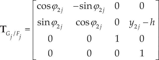
Finally, the position and orientation of the frame H_j (which is attached to the hip as shown in Figure 1) relative to the frame G_j is,

$$T_{H_j/G_j}=\left[\begin{array}{cccc}\cos {\theta }_j& 0& \sin {\theta }_j& 0\\ 0& 1& 0& 0\\ -\sin {\theta }_j& 0& \cos {\theta }_j& 0\\ 0& 0& 0& 1\end{array}\right]$$

(7)

where θ _j is the angle that the frame G_j must be rotated about its Y axis to align the axes of the coordinate frames G_j and H_j. The position and orientation of the hip relative to the foot j can be obtained multiplying the previous three matrices:

$$T_{H_j/E_j}=T_{F_j/E_j}{T}_{G_j/F_j}{T}_{H_j/G_j}$$

(8)

The matrix T_{H j /E j} has the following expression,

$$T_{H_j/E_j}=\left[\begin{array}{cccc}{c}_{{\theta }_j}{c}_j& s_j& s_{{\theta }_j}{c}_j& y_j{s}_{{\phi }_{1j}}\\ -c_{{\theta }_j}{s}_j& c_j& -s_{{\theta }_j}{s}_j& y_j{c}_{{\phi }_{1j}}\\ -s_{{\theta }_j}& 0& c_{{\theta }_j}& 0\\ 0& 0& 0& 1\end{array}\right]$$

(9)

where y _j is defined in Eq. (4) and the following variables have been used to abbreviate the trigonometric functions: $s_{{\theta }_j}=\sin {\theta }_j$ , $c_{{\theta }_j}=\cos {\theta }_j$ , $s_{{\phi }_{1j}}=\sin {\phi }_{1j}$ , $c_{{\phi }_{1j}}=\cos {\phi }_{1j}$ , $s_j=\sin ({\phi }_{1j}-{\phi }_{2j})$ , $c_j=\cos ({\phi }_{1j}-{\phi }_{2j})$ .

Particularizing the matrix T_{H j /E j} for the two legs (j = A and j = B), the relative position and orientation between the frames attached to the feet can be obtained performing the following product,

$$T_{E_B/E_A}=T_{H_A/E_A}{T}_{H_B/H_A}{T}_{E_B/H_B}$$

(10)

where $T_{E_B/H_B}={\left(T_{H_B/E_B}\right)}^{-1}$ and $T_{H_B/H_A}$ is the matrix that encodes the position and orientation of the frame H_B with respect to the frame H_A,

$$T_{H_B/H_A}=\left[\begin{array}{cccc}1& 0& 0& t\\ 0& 1& 0& 0\\ 0& 0& 1& 0\\ 0& 0& 0& 1\end{array}\right]$$

(11)

which is constant because both coordinate frames are attached to the same link (the hip). t > 0 is the distance between the parallel rotation axes of the hip (see Figure 1).

Equation (10) provides the solution to the forward kinematics of the complete robot. If the 10 joint coordinates are known, the solution to the forward kinematics of the parallel mechanisms (which can be found in [21, 22]) yields the values of the intermediate joint coordinates. Substituting the intermediate joint coordinates into Eq. (10) gives the matrix T_{E B /E A} , which encodes the relative position and orientation between the feet of the robot.

The inverse problem is necessary to plan the movements of the robot: finding the values of the intermediate joint coordinates necessary to achieve a desired position and orientation T_{E B /E A} . This problem is addressed next.

4.2 Solution to the inverse kinematics

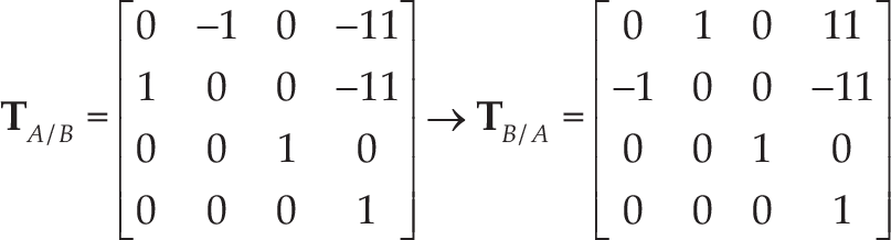
In this section, we will calculate the values of the 10 intermediate joint coordinates necessary to reach a desired position and orientation between the feet of the robot. Without loss of generality, it will be assumed that the input to the inverse kinematics is the matrix T_{E B /E A} , which encodes the position and orientation of the foot B relative to the foot A. If the input is T_{E A /E B} , one only needs to invert this matrix to obtain T_{E B /E A} , which can be directly used in the equations that will be derived in this section. It will be assumed that the input matrix has the following form:

$$T_{E_B/E_A}=\left[\begin{array}{cccc}{r}_{11}& r_{12}& r_{13}& p_x\\ r_{21}& r_{22}& r_{23}& p_y\\ r_{31}& r_{32}& r_{33}& p_z\\ 0& 0& 0& 1\end{array}\right]$$

(12)

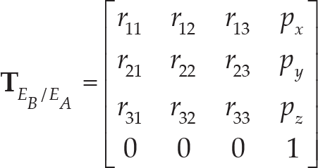
Inserting the previous matrix into Eq. (10) yields a system of equations from which the intermediate joint coordinates, which appear on the right-hand side of Eq. (10), must be solved. Trying to solve Eq. (10) directly can be difficult because all the unknowns are coupled on its right-hand side, and the resulting equations are quite large and difficult to handle. However, if Eq. (10) is post-multiplied by $T_{H_B/E_B}={\left(T_{E_B/H_B}\right)}^{-1}$ , it becomes:

$$T_{E_B/E_A}{T}_{H_B/E_B}=T_{H_A/E_A}{T}_{H_B/H_A}$$

(13)

Thus, the problem becomes easier, since the unknowns associated with each leg have been decoupled and appear on different sides of the equation. Indeed, the matrix on the left-hand side of Eq. (13) only depends on the variables of the leg B{y_B,φ_1B,φ_2B,θ _B }, whereas the right-hand side only depends on the variables of the leg A{y_A,φ_1A,φ_2A,θ _A }. In what follows, the left-hand side of Eq. (13) will be denoted by B, whereas the right-hand side will be denoted by A. The expressions of these matrices, which involve much simpler terms than the right-hand side of Eq. (10), can be found in Eqs. (14) and (15).

$$B=\left[\begin{array}{cccc}{c}_{{\theta }_B}(c_B{r}_{11}-s_B{r}_{12})-r_{13}{s}_{{\theta }_B}& s_B{r}_{11}+c_B{r}_{12}& s_{{\theta }_B}(c_B{r}_{11}-s_B{r}_{12})+r_{13}{c}_{{\theta }_B}& r_{11}{y}_B{s}_{{\phi }_{1B}}+r_{12}{y}_B{c}_{{\phi }_{1B}}+p_x\\ c_{{\theta }_B}(c_B{r}_{21}-s_B{r}_{22})-r_{23}{s}_{{\theta }_B}& s_B{r}_{21}+c_B{r}_{22}& s_{{\theta }_B}(c_B{r}_{21}-s_B{r}_{22})+r_{23}{c}_{{\theta }_B}& r_{21}{y}_B{s}_{{\phi }_{1B}}+r_{22}{y}_B{c}_{{\phi }_{1B}}+p_y\\ c_{{\theta }_B}(c_B{r}_{31}-s_B{r}_{32})-r_{33}{s}_{{\theta }_B}& s_B{r}_{31}+c_B{r}_{32}& s_{{\theta }_B}(c_B{r}_{31}-s_B{r}_{32})+r_{33}{c}_{{\theta }_B}& r_{31}{y}_B{s}_{{\phi }_{1B}}+r_{32}{y}_B{c}_{{\phi }_{1B}}+p_z\\ 0& 0& 0& 1\end{array}\right]$$

(14)

$$A=\left[\begin{array}{cccc}{c}_{{\theta }_A}{c}_A& s_A& s_{{\theta }_A}{c}_A& y_A{s}_{{\phi }_{1A}}+t{c}_{{\theta }_A}{c}_A\\ -c_{{\theta }_A}{s}_A& c_A& -s_{{\theta }_A}{s}_A& y_A{c}_{{\phi }_{1A}}-t{c}_{{\theta }_A}{s}_A\\ -s_{{\theta }_A}& 0& c_{{\theta }_A}& -t{s}_{{\theta }_A}\\ 0& 0& 0& 1\end{array}\right]$$

(15)

To solve the inverse kinematics, we must solve the equations that are obtained when all the elements of the matrix A are equated to the respective elements of the matrix B. Equating the elements (1,4), (2,4) and (3,4) of both matrices yields the following equations:

$$y_A{s}_{{\phi }_{1A}}+t{c}_{{\theta }_A}{c}_A=r_{11}{y}_B{s}_{{\phi }_{1B}}+r_{12}{y}_B{c}_{{\phi }_{1B}}+p_x$$

(16)

$$y_A{c}_{{\phi }_{1A}}-t{c}_{{\theta }_A}{s}_A=r_{21}{y}_B{s}_{{\phi }_{1B}}+r_{22}{y}_B{c}_{{\phi }_{1B}}+p_y$$

(17)

$$-t{s}_{{\theta }_A}=r_{31}{y}_B{s}_{{\phi }_{1B}}+r_{32}{y}_B{c}_{{\phi }_{1B}}+p_z$$

(18)

Equating the elements (1,2), (2,2), (3,1), (3,3) and (3,2) gives the following equations:

$$s_A=s_B{r}_{11}+c_B{r}_{12}$$

(19)

$$c_A=s_B{r}_{21}+c_B{r}_{22}$$

(20)

$$s_{{\theta }_A}=r_{33}{s}_{{\theta }_B}-c_{{\theta }_B}(c_B{r}_{31}-s_B{r}_{32})$$

(21)

$$c_{{\theta }_A}=r_{33}{c}_{{\theta }_B}+s_{{\theta }_B}(c_B{r}_{31}-s_B{r}_{32})$$

(22)

$$0=s_B{r}_{31}+c_B{r}_{32}$$

(23)

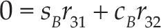
It can be shown (see Appendix A) that, if Eqs. (19) to (23) are satisfied, the elements (1,1), (1,3), (2,1) and (2,3) of A and B are equal. Hence, the equations that are obtained equating these elements of both matrices must not be included since they depend on Eqs. (19) to (23), and we only need to solve Eqs. (16) to (23). These equations are solved next, distinguishing two cases.

4.3 Case 1: (r₃₁, r₃₂)≠(0,0)

In this case, r₃₁² + r₃₂² ≠ 0 and Eq. (23) can be solved together with the condition s_B² + c_B² = 1, obtaining two solutions for s_B and c_B,

$$s_B=\sin ({\phi }_{1B}-{\phi }_{2B})={\sigma }_1\frac{r_{32}}{\sqrt{r_{31}^2+r_{32}^2}}$$

(24)

$$c_B=\cos ({\phi }_{1B}-{\phi }_{2B})={\sigma }_1\frac{-r_{31}}{\sqrt{r_{31}^2+r_{32}^2}}$$

(25)

where σ₁ ∊ {−1,1}. Since s_B and c_B are known, the difference φ_1B − φ_2B can be calculated as follows:

$${\phi }_{1B}-{\phi }_{2B}=atan2(s_B\mathrm{,}{c}_B)$$

(26)

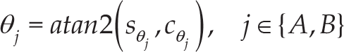
where atan2 is the well-known inverse tangent function that considers the signs of the sine and the cosine and computes the angle in the correct quadrant. Equation (26) gives φ_2B in terms of φ_1B. After calculating s_B and c_B, s_A and c_A are calculated from Eqs. (19) and (20), respectively. Next, the difference φ_1A − φ_2A is obtained as follows,

$${\phi }_{1A}-{\phi }_{2A}=\mathrm{atan}2\left(s_A\mathrm{,}{c}_A\right)$$

(27)

which provides φ_2A in terms of φ_1A. Once s_A and c_A are known, Eqs. (16) to (18) constitute a system of three equations with five unknowns: {φ_1B,φ_1A,y _B ,y _A ,θ _A }. Hence, three unknowns must be solved in terms of the other two, which must be assumed to be known. From the form of these equations, it is evident that the solution is straightforward if y_B and φ_1B are chosen as the known variables, since in this case the right-hand side of the equations is known. Particularly, Eq. (18) yields sinθ _A :

$$s_{{\theta }_A}=-\frac{r_{31}{y}_B{s}_{{\phi }_{1B}}+r_{32}{y}_B{c}_{{\phi }_{1B}}+p_z}{t}$$

(28)

Note that the right-hand side of Eq. (28) must be in [−1,1] in order to obtain a real value for θ _A . Knowing the value of s_{θ A} , two solutions are obtained for cosθ _A ,

$$c_{{\theta }_A}={\sigma }_2\sqrt{1-s_{{\theta }_A}^2}$$

(29)

where σ₂ ∊ {−1,1}. Once s_{θ A} and c_{θ A} are known, s_{θ B} and c_{θ B} are calculated inverting Eqs. (21) and (22), which can always be inverted (see Appendix B). The solution for s_{θ B} and c_{θ B} is:

$$s_{{\theta }_B}=r_{33}{s}_{{\theta }_A}+c_{{\theta }_A}(c_B{r}_{31}-s_B{r}_{32})$$

(30)

$$c_{{\theta }_B}=r_{33}{c}_{{\theta }_A}-s_{{\theta }_A}(c_B{r}_{31}-s_B{r}_{32})$$

(31)

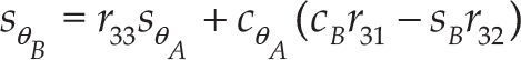
As such, θ _A and θ _B are obtained as follows:

$${\theta }_j=atan2\left(s_{{\theta }_j}\mathrm{,}{c}_{{\theta }_j}\right)\mathrm{,}j\in \left\{A\mathrm{,}B\right\}$$

(32)

After c_θA has been calculated, Eqs. (16) and (17) can be rewritten as follows,

$$y_A{s}_{{\phi }_{1A}}={\mathrm{\Omega }}_x$$

(33)

$$y_A{c}_{{\phi }_{1A}}={\mathrm{\Omega }}_y$$

(34)

where the terms Ω _x and Ω _y , on the right-hand side of the equations, are known quantities:

$${\mathrm{\Omega }}_x=r_{11}{y}_B{s}_{{\phi }_{1B}}+r_{12}{y}_B{c}_{{\phi }_{1B}}+p_x-t{c}_{{\theta }_A}{c}_A$$

(35)

$${\mathrm{\Omega }}_y=r_{21}{y}_B{s}_{{\phi }_{1B}}+r_{22}{y}_B{c}_{{\phi }_{1B}}+p_y+t{c}_{{\theta }_A}{s}_A$$

(36)

Squaring Eqs. (33) and (34) and adding them together eliminates φ_1A and yields the following solution for y_A:

$$y_A=\pm \sqrt{{\mathrm{\Omega }}_x^2+{\mathrm{\Omega }}_y^2}$$

(37)

After calculating y_A, φ_1A is obtained as follows,

$${\phi }_{1A}=atan2\left({\mathrm{\Omega }}_x/y_A\mathrm{,}{\mathrm{\Omega }}_y/y_A\right)$$

(38)

which is valid only if y_A ≠ 0. Note, however, that the case y_A ≤ 0 will be impossible in practice due to mechanical interference between different links of the leg A. Hence, we will be interested only in strictly positive solutions of y_A, given by the positive sign in Eq. (37). In that case, y_A can be removed from Eq. (38) because an angle is not affected if its sine and cosine are multiplied by the same positive constant (whereas multiplying them by a negative constant is equivalent to adding π rad to the angle). Hence, φ_1A can be directly obtained as follows:

$${\phi }_{1A}=atan2\left({\mathrm{\Omega }}_x\mathrm{,}{\mathrm{\Omega }}_y\right)$$

(39)

With the obtained value of φ_1A, φ_2A is calculated using Eq. (27). Finally, φ_2B is calculated from φ_1B (which is assumed to be known) using Eq. (26).

Note that the variables y_1A and y_1B remain undetermined after solving all the equations. Hence, the values of these intermediate joint coordinates must also be fixed in order to complete the solution to the inverse kinematics. Assuming that the values of these variables are known, the solution to the inverse kinematics can be summarized as follows,

$$\begin{array}{l}\left\{y_A\mathrm{,}{\phi }_{1A}\mathrm{,}{\phi }_{2A}\mathrm{,}{\phi }_{2B}\mathrm{,}{\theta }_A\mathrm{,}{\theta }_B\right\}=f_1\left({\phi }_{1B}\mathrm{,}{y}_B\right)\\ \left\{{\phi }_{1B}\mathrm{,}{y}_B\mathrm{,}{y}_{1A}\mathrm{,}{y}_{1B}\right\}=\text{\hspace{0.05em}free parameters\hspace{0.05em}}\end{array}$$

(40)

where the symbol f₁ indicates that the variables on the left-hand side of Eq. (40) are obtained from {φ_1B,y_B}, as described in this section.

4.4 Case 2: r₃₁=r₃₂=0

Since r₃₁² + r₃₂² + r₃₃² = 1, the condition r₃₁ = r₃₂ = 0 is equivalent to r₃₃² = 1, which means that the Z axes of the coordinate frames attached to the feet are parallel. This situation appears in many simple movements of the robot when exploring a structure, such as in concave and convex transitions between different planes (see Section 6).

This case admits a similar analysis to the previous one: some unknowns must be solved in terms of the others and, in particular, we can choose to solve all the unknowns in terms of the variables φ_1B and y_B to deal with simpler equations. However, since r₃₁ = r₃₂ = 0, a restriction is lost because Eq. (23) is identically satisfied. Thus, the difference φ_1B − φ_2B is no longer fixed and can adopt any value, which means that the value of the variable φ_2B must also be decided. Except for this difference, the resolution procedure is exactly as described in the previous section: we fix the values of {y_B,φ_1B,φ_2B}, compute s_B = sin(φ_1B − φ_2B) and c_B = cos(φ_1B − φ_2B), and use Eqs. (27) to (39) to calculate the rest of the variables.

As in Case 1, the values of the variables y_1A and y_1B must be fixed since they remain undetermined after solving the equations. Thus, in this case, the solution to the inverse kinematics can be summarized as follows,

$$\begin{array}{l}\left\{y_A\mathrm{,}{\phi }_{1A}\mathrm{,}{\phi }_{2A}\mathrm{,}{\theta }_A\mathrm{,}{\theta }_B\right\}=f_2\left({\phi }_{1B}\mathrm{,}{\phi }_{2B}\mathrm{,}{y}_B\right)\\ \left\{{\phi }_{1B}\mathrm{,}{\phi }_{2B}\mathrm{,}{y}_B\mathrm{,}{y}_{1A}\mathrm{,}{y}_{1B}\right\}=\text{\hspace{0.05em}free parameters\hspace{0.05em}}\end{array}$$

(41)

where the symbol f₂ indicates that the variables on the left-hand side of Eq. (41) are obtained from {φ_1B,φ_2B,y_B}, as described in this section.

4.5 Geometric interpretation: self-motion sets

For non-redundant robots, the solution to the inverse kinematics for a desired position and orientation is a set of isolated points in the space of the joint coordinates (the joint space). However, for redundant robots, the values of the joint coordinates that permit the robot to reach a desired position and orientation lie in positive-dimensional sets (curves, surfaces, etc.) in the joint space. These sets are called self-motion sets because varying the joint coordinates along them modifies the posture of the robot without affecting the position and orientation of its end-effector, which remains motionless [23, 24].

For this robot, the solutions to the inverse kinematics can be interpreted as self-motion sets in the 10D space of the intermediate joint coordinates. In Case 1, the solutions lie in a 4D set because the solution is parameterized in terms of four parameters, and Eq. (40) provides a possible parametrization of the self-motion set. In Case 2, the dimension of the self-motion set is five, since five parameters must be fixed in order to determine all the intermediate joint coordinates. In this case, a possible parametrization of the self-motion set is given by Eq. (41).

Note that Eqs. (40) and (41) are not the only valid parametrizations of the self-motion sets. There are many other parametrizations, depending on the redundant variables that are assumed to be known when solving the equations for the inverse kinematics. For example, instead of choosing {y_B,φ_1B}, we could have chosen {φ_1A,φ_1B} or {y_A,y_B} as the known variables to solve three unknowns from Eqs. (16) to (18). In these cases, however, it is evident that the solution to the equations is not as straightforward as when {y_B,φ_1B} are chosen as the known variables.

Although the self-motion sets encode all the information regarding the solution to the inverse kinematics of redundant robots, the self-motion sets obtained for this robot are not practical due to their high dimensionality. In the next section, we propose a more useful representation of the solutions to the inverse kinematics of the studied climbing robot.

5. Inverse kinematics: Regions of feasible solutions

In the previous section, it was shown that the solution to the inverse kinematics can be written in terms of some free parameters or decision variables whose values must be decided: {φ_1B,y_B,y_1A,y_1B} (and also φ_2B, in Case 2). This section discusses how to choose appropriate values for these decision variables.

First, note that the chosen values should satisfy the joint limits of the parallel mechanisms. As shown in Section 3, these joint limits impose restrictions on the variables (φ _ij ,y_ij) of the parallel mechanisms. In this regard, it will be assumed that the valid pairs (φ _ij ,y_ij) of each parallel mechanism belong to a region of the form of Eq. (3).

Taking the joint limits into consideration, the best representation of the solutions to the inverse kinematics of this robot would be the combinations of the decision variables {φ_1B,y_B,y_1A,y_1B} (and also φ_2B, in Case 2) that yield a desired position and orientation between the feet while satisfying the joint limits of the parallel mechanisms. This representation would consist of the regions of feasible combinations of these variables in a 4D or 5D space. However, as is shown next, it is possible to encode the most relevant information of these feasible regions using only two or three dimensions.

Note that the posture of the robot is not affected by all the decision variables equally. According to Eqs. (40) and (41), fixing all the decision variables except {y_1A,y_1B} fixes the remaining intermediate joint coordinates which determine the posture of the robot. Once y _j has been fixed, varying y_1j only modifies the position of the core link C _j along the leg j, without affecting the posture of the robot. This is because a variation in y_1j will be compensated by the opposite variation in the variable y_2j to conserve the value of y_j, which has already been fixed (see Figure 5).

Since the variables {y_1A, y_1B} do not affect the overall posture of the robot (except for the position of the core links along the legs), their concrete values are not important as long as they satisfy the joint limits of the parallel mechanisms. Thus, it suffices to focus only on the decision variables {φ_1B,φ_2B,y_B}, which determine the overall posture of the robot and are important for planning its movements (e.g., for choosing the postures that yield a desired position and orientation avoiding some obstacles).

For Case 1, we are interested in the regions (areas) R_f of the (φ_1B,y_B) plane for which we can find values for the other decision variables (y_1A and y_1B) that permit the robot to reach a desired position and orientation satisfying the joint limits. A discrete approximation of these areas can be obtained using Algorithm 1. This algorithm picks N_p random points in the (φ_1B,y_B) plane, computes the intermediate joint coordinates {y_A,φ_1A,φ_2A,φ_2B,θ _A ,θ _B } for each point using the equations of Section 4.3, and discards all the points for which the intermediate joint coordinates do not satisfy the joint limits of the parallel mechanisms. According to Section 3, it is necessary that the angles {φ_1B,φ_2B,φ_1A,φ_2A} be in [φ _min ,φ _max ] for a point to satisfy the joint limits. Moreover, y_j (j ∊ {A,B}) must be in $[\underset{\_}{y_j}\mathrm{,}\overline{y_j}]$ , where the bounds $\underset{\_}{y_j}$ and $\overline{y_j}$ are calculated using Eq. (4) and the bounds of the variables y_1j and y_2j, which depend on φ_1j and φ_2j, respectively.

Algorithm 1.

Algorithm to compute the set R_f of feasible solutions to the inverse kinematics which satisfy the joint limits of the parallel mechanisms.

For Case 2, we are interested in the regions (volumes) R_f of the (φ_1B,φ_2B,y_B) space for which we can find values of the decision variables {y_1A,y_1B} that permit the robot to reach a desired position and orientation satisfying the joint limits. Algorithm 1 can also be used to compute a discrete approximation of these volumes. The only difference is in Line 4 of the algorithm: instead of calculating φ_2B from Eq. (26), the value of φ_2B must be sampled uniformly on [φ _min ,φ _max ] because φ_2B cannot be calculated in terms of φ_1B in Case 2. Moreover, the points that are stored in R_f at Line 17 have three coordinates instead of two: (φ_1B,φ_2B,y_B).

Note that the solution to the inverse kinematics in Case 1 involves two binary variables σ₁,σ₂ ∊ {−1,1}. The solution in Case 2 involves only the binary variable σ₂. Thus, the regions R_f computed by Algorithm 1 will be different for different choices of these binary variables. In both Cases 1 and 2, it is necessary to execute the algorithm for all the combinations of the binary variables to avoid missing feasible solutions to the inverse kinematics.

All the points calculated by Algorithm 1 guarantee the existence of values for the decision variables y_1A and y_1B that satisfy the joint limits, as demonstrated in the next subsection 5.1.

As an alternative to the numerical algorithm presented in this section, one might try to compute the regions R_f or redundant solutions analytically. To obtain analytic representations of these regions, it suffices to obtain analytically the curves (or surfaces, in Case 2) that enclose these regions. This can be done solving Eqs. (27) to (39) to find analytic expressions of all the intermediate joint coordinates in terms of φ_1B and y_B (and also φ_2B, in Case 2). Next, equating each intermediate joint coordinate to either its upper or lower limit yields an equation that defines a curve in the (φ_1B, y _B ) plane or a surface in the (φ_1B,φ_2B,y_B) space, and these curves/surfaces constitute the limits of the regions R_f. Note that the lower and upper limits of φ _ij are constants, φ _min and φ _max , respectively. However, according to Algorithm 1, the bounds of y_j depend on φ _ij , which, in turn, must be written in terms of {φ_1B,φ_2B,y_B}.

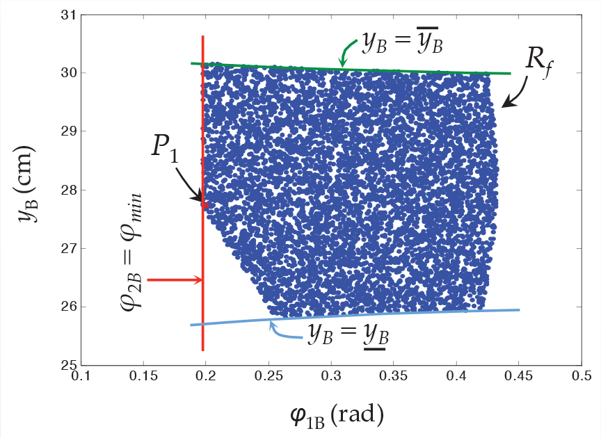
Unfortunately, obtaining analytically all the intermediate joint coordinates and the bounds of y_j in terms of {φ_1B,φ_2B,y_B} can be very difficult or even not feasible - even using computer algebra systems - due to the large size and complexity of the analytic expressions that must be handled in the calculations. For instance, Figure 7 shows an example of the region R_f computed using Algorithm 1, and it also shows some of the curves that delimit this region. Only the boundaries that could be obtained analytically are shown; the analytic expressions of the remaining boundaries of R_f could not be obtained due to the complexity and large size of the terms involved in their calculation. Thus, for this robot, an analytic approach to compute the sets of redundant solutions for the inverse kinematics is intractable, and a numerical algorithm like the one proposed in this section stands as the best choice.

5.1 Choosing the values of y_1A and y_1B

The regions R_f of the feasible solutions computed by Algorithm 1 only reflect the valid combinations of the variables φ_1B and y_B (and φ_2B, in Case 2). However, the values of the variables y_1A and y_1B must also be decided in order to complete the solution for the inverse kinematics.

As discussed in the previous section, since the variables {y_1A,y_1B} do not affect the posture of the robot once {y _A ,y _B } are fixed, their values are not crucial as long as they satisfy the joint limits. Next, it will be shown that, for every point in R_f, we can always find non-empty intervals for the variables y_1A and y_1B that satisfy the joint limits of the parallel mechanisms. This will be demonstrated for a generic variable y_1j (j ∊ {A,B}).

According to Eq. (3), for a given φ_1j ∊ [φ _min ,φ _max ] y_1j must be in $[\underset{\_}{y_{1j}}({\phi }_{1j})\mathrm{,}\overline{y_{1j}}({\phi }_{1j})]$ . Additionally, y_1j must also satisfy Eq. (4):

$$y_{2j}=y_j+h-y_{1j}$$

(42)

Similarly, for a given φ_2j ∊ [φ _min ,φ _max ], y_2j must satisfy:

$$\underset{\_}{y_{2j}}({\phi }_{2j})\le y_{2j}\le \overline{y_{2j}}({\phi }_{2j})$$

(43)

Combining the conditions given in Eqs. (42) and (43) yields the following additional bounds for y_1j:

$$y_j+h-\overline{y_{2j}}({\phi }_{2j})\le y_{1j}\le y_j+h-\underset{\_}{y_{2j}}({\phi }_{2j})$$

(44)

Hence, the valid values of y_1j lie in the intersection of the two intervals $I_1=[\underset{\_}{y_{1j}}({\phi }_{1j})\mathrm{,}\overline{y_{1j}}({\phi }_{1j})]$ and $I_2=[y_j+h-\overline{y_{2j}}({\phi }_{2j})\mathrm{,}{y}_j+h-\underset{\_}{y_{2j}}({\phi }_{2j})]$ . Denoting the limits of these intervals by $I_1=[a_0\mathrm{,}{a}_1]$ and $I_2=[b_0\mathrm{,}{b}_1]$ , their intersection will be empty if, and only if, [25]:

$$b_1-a_0<0\text{\hspace{1em}\hspace{0.05em}OR\hspace{0.05em}\hspace{1em}}{b}_0-a_1>0$$

(45)

Next, applying De Morgan's laws to the previous condition, the intersection I₁ ∩ I₂ will be non-empty if, and only if:

$$b_1-a_0\ge 0\text{\hspace{1em}\hspace{0.05em}AND\hspace{0.05em}\hspace{1em}}{b}_0-a_1\le 0$$

(46)

First, we check the first condition of Eq. (46),

$$\begin{array}{l}{b}_1-a_0=y_j+h-\underset{\_}{y_{2j}}({\phi }_{2j})-\underset{\_}{y_{1j}}({\phi }_{1j})\ge \\ \underset{\_}{y_{1j}}({\phi }_{1j})+\underset{\_}{y_{2j}}({\phi }_{2j})-h+h-\underset{\_}{y_{2j}}({\phi }_{2j})-\underset{\_}{y_{1j}}({\phi }_{1j})=0\end{array}$$

(47)

where it has been considered that $y_j\ge \underset{\_}{y_{1j}}({\phi }_{1j})+\underset{\_}{y_{2j}}({\phi }_{2j})-h$ , which is guaranteed by Algorithm 1. Next, we check the second condition of Eq. (46),

$$\begin{array}{l}{b}_0-a_1=y_j+h-\overline{y_{2j}}({\phi }_{2j})-\overline{y_{1j}}({\phi }_{1j})\le \\ \overline{y_{1j}}({\phi }_{1j})+\overline{y_{2j}}({\phi }_{2j})-h+h-\overline{y_{2j}}({\phi }_{2j})-\overline{y_{1j}}({\phi }_{1j})=0\end{array}$$

(48)

where it has been considered that $y_j\le \overline{y_{1j}}({\phi }_{1j})+\overline{y_{2j}}({\phi }_{2j})-h$ , which is also guaranteed by Algorithm 1. Thus, it is guaranteed that, for every point of the sets R_f computed by the proposed algorithm, we can always find ranges of the variables y_1A and y_1B that satisfy the joint limits of the parallel mechanisms.

6. Examples

This section presents some examples of the application of Algorithm 1 to obtain the region R_f of the valid solutions to the inverse kinematics. Algorithm 1 was implemented in MATLAB R2011b and the examples were tested on a laptop Acer Travelmate 5720, with an Intel(R) Core(TM)2 Duo T7300 CPU @ 2 GHz, 2 GB of RAM, and a 32-bit Operating System (Windows 7 Professional).

For the geometric parameters of the parallel mechanisms {b,p,ρ₀,Δρ}, the values indicated in Section 3 were used. For the parameters {h,t}, the following values were used: h = 16 cm and t = 15.6 cm, which correspond to the design shown in Figure 1.

Example 1. It is assumed that the foot A is fixed, and the following position and orientation are desired for the foot B:

$$T_{B/A}=\left[\begin{array}{cccc}0& 0& -1& -20cm\\ \sin (\pi /3)& \cos (\pi /3)& 0& 5cm\\ \cos (\pi /3)& -\sin (\pi /3)& 0& 30cm\\ 0& 0& 0& 1\end{array}\right]$$

(49)

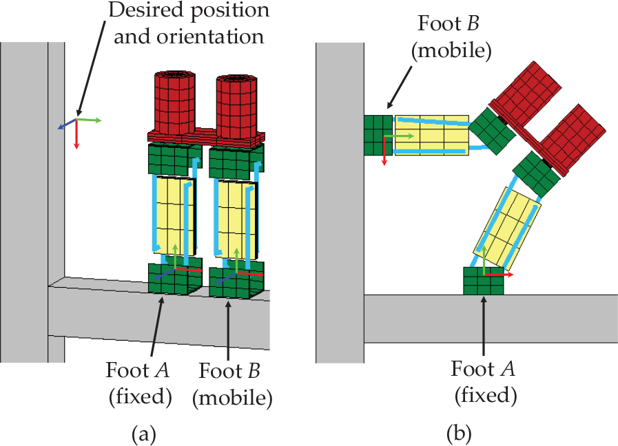
This example is represented in Figure 6a. Since (r₃₁,r₃₂)≠(0,0), two binary variables σ₁,σ₂ ∊ {−1,1} are involved in the calculation of the intermediate joint coordinates, as explained in Section 4.3. Hence, in order to obtain all the feasible solutions, Algorithm 1 must be executed four times, once for each combination of these binary variables. The set R_f of feasible solutions depends on the choice of the binary variables.

For this example, Algorithm 1 was run using N_p = 10⁴ and N_p = 5 ⋅ 10⁴ random points. In the first case, the average time of execution of the algorithm was 0.455 s, with a standard deviation (SD) of 0.022 s. For N_p = 5 ⋅ 10⁴, the average execution time was 2.35 s, with an SD of 0.12 s. In each case, 20 experiments were performed.

In both cases, these are the times necessary to run the algorithm four times, once for each combination of σ₁ and σ₂. The only combination of σ₁ and σ₂ that yields a non-empty set of feasible solutions for this example is σ₁ = σ₂ = − 1. The set R_f corresponding to this combination is shown in Figure 7. Figure 7 represents only the solution obtained for N = 5 ⋅ 10⁴ since the density of the points is higher, providing a better approximation of the shape of the region of feasible solutions.

Figure 6.

Desired position and orientation in Example 1

Figure 7.

Discrete approximation of the set R_f of feasible solutions to the inverse kinematics in Example 1 for N_p=5⋅10⁴ points

As shown in the previous section, any point of the region R_f guarantees the existence of ranges for y_1A and y_1B that allow the robot to reach the position and orientation of Eq. (49), satisfying the joint limits of the parallel mechanisms. For example, the point P₁ = (0.2,27.75) indicated in Figure 7 yields θ _A = −2.51 rad and θ _B = −0.94 rad. For this point, the valid ranges of y_1A and y_1B are [20.21,20.31] cm and 121.79,21.80] cm, respectively (the values are rounded to two decimal places). These ranges are very narrow because P₁ is close to the boundary of R_f. Choosing y_1A=20.21 cm and y_1B = 21.79 cm gives the following values for the joint coordinates of the parallel mechanisms,

$$\begin{array}{l}{u}_{1A}=\mathrm{21.42,}{v}_{1A}=\mathrm{19.00,}{u}_{2A}=\mathrm{21.52,}{v}_{2A}=19.10\\ u_{1B}=\mathrm{21.00,}{v}_{1B}=\mathrm{22.59,}{u}_{2B}=\mathrm{24.99,}{v}_{2B}=19.01\end{array}$$

(50)

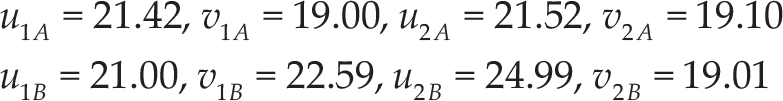
where the values are in cm and rounded to two decimal places. Note that some lengths are close to the joint limits (19 and 25 cm), which agrees with the fact that P₁ is close to the boundary of R_f. This solution yields the posture shown in Figure 6b.

Example 2. In this example, the foot A is fixed and the foot B must reach the following position and orientation to perform a concave transition between two planes (see Figure 8):

$$T_{B/A}=\left[\begin{array}{cccc}0& 1& 0& -25cm\\ -1& 0& 0& 35cm\\ 0& 0& 1& 0cm\\ 0& 0& 0& 1\end{array}\right]$$

(51)

According to Section 4.4, since r₃₁ = r₃₂ = 0, only the binary variable σ₂ is involved in the calculation of the intermediate joint coordinates. Thus, Algorithm 1 must be executed twice to obtain all the feasible solutions, once for each value of σ₂ ∊ {−1,1}.

For this example, Algorithm 1 was run for N _p = 10⁴ and N_p = 5 ⋅ 10⁴ random points, obtaining the following average execution times: 1.04 s (SD =0.05 s) and 5.19 s (SD = 0.24 s) (20 experiments were performed in both cases). These are the times necessary to run the algorithm twice (once for each value of σ₂) in order to find all the feasible solutions.

In this example, only σ₂ = −1 yields a non-empty set of feasible solutions, which is shown in Figure 9. The set represented in Figure 9 is the one obtained for N_p = 5 ⋅ 10⁴ points, which provides a better approximation of the solution set. The projections of the solution set onto the coordinate planes have also been represented, so that its 3D shape can be observed more easily.

Figure 8.

Desired position and orientation in Example 2, where the robot performs a concave transition between two planes

For example, choosing the point P₂=(0,0.8,26), which is represented in Figure 9 (along with its projections onto the coordinate planes), yields the following ranges for y_1A and y_1B: [20.80,22.84] cm and [19.90,20.16] cm, respectively. Choosing y_1A = 21 cm and y_1B = 20 cm yields the following joint coordinates (values in cm),

$$\begin{array}{l}{u}_{1A}=\mathrm{19.20,}{v}_{1A}=\mathrm{22.81,}{u}_{2A}=\mathrm{23.23,}{v}_{2A}=20.84\\ u_{1B}=\mathrm{20.00,}{v}_{1B}=\mathrm{20.00,}{u}_{2B}=\mathrm{19.17,}{v}_{2B}=24.90\end{array}$$

(52)

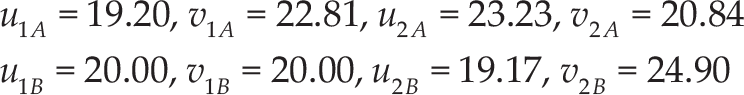
where some joint coordinates are close to the joint limits because the range of valid values of y_1B for the chosen point P₂ is very narrow. This solution yields the posture shown in Figure 8b. For this example, the rotations of the hip are: θ _A = θ _B = π rad. Note that the rotations of the hip do not depend on the decision variables when r₃₁ = r₃₂ = 0, as can be observed in Eqs. (28) to (31).

Figure 9.

Figure 9. Set R_f of feasible solutions for the inverse kinematics in Example 2, for N_p = 5⋅10⁴ points

Example 3. In this case, the foot B is fixed and the foot A must reach the following position and orientation to perform a convex transition between two planes (see Figure 10),

$$T_{A/B}=\left[\begin{array}{cccc}0& -1& 0& -11\\ 1& 0& 0& -11\\ 0& 0& 1& 0\\ 0& 0& 0& 1\end{array}\right]\to T_{B/A}=\left[\begin{array}{cccc}0& 1& 0& 11\\ -1& 0& 0& -11\\ 0& 0& 1& 0\\ 0& 0& 0& 1\end{array}\right]$$

(53)

where the position is given in cm. The matrix T_A/B must be inverted to obtain T_B/A, which is the input to the inverse kinematic problem as formulated in Section 4.2.

As in Example 2, since r₃₁ = r₃₂ = 0, Algorithm 1 must be run twice. In this example, the algorithm was also tested for N_p = 10⁴ and N_p = 5⋅10⁴ random points, obtaining the following average execution times for 20 experiments in each case: 0.919 s (SD = 0.003 s) and 4.47 s (SD = 0.20 s), respectively. Again, these are the times necessary to run the algorithm twice: for σ₂ = −1 and σ₂ = 1. In this example, only σ₂ = l yields a non-empty set of feasible solutions, which is shown in Figure 11 for N_p = 5 ⋅ 10⁴ points. As in the previous example, the projections of the solution set onto the coordinate planes are also shown to facilitate the 3D visualization of the shape of R_f.

Figure 10.

Desired position and orientation in Example 3, where the robot performs a convex transition between two planes

Figure 11.

Set R_f of feasible solutions for the inverse kinematics in Example 3, for N_p=5⋅10⁴ points

For example, choosing the point P₃ = (−0.8, −0.2, 26), shown in Figure 11, yields the following ranges for y_1A and y_1B: [21.78,22.16] cm and [21.84,22.10] cm, respectively. Choosing y_1A = y_1B = 22 cm gives the following lengths,

$$\begin{array}{l}{u}_{1A}=\mathrm{19.22,}{v}_{1A}=\mathrm{24.84,}{u}_{2A}=\mathrm{23.63,}{v}_{2A}=22.11\\ u_{1B}=\mathrm{24.90,}{v}_{1B}=\mathrm{19.17,}{u}_{2B}=\mathrm{20.80,}{v}_{2B}=19.21\end{array}$$

(54)

where the values are in cm. For this solution, the robot has the posture shown in Figure 10b. For this example, the rotations of the hip are: θ _A = θ _B = 0 (independently of the decision variables because r₃₁ = r₃₂ = 0).

7. Conclusions and future work

This paper has presented the inverse kinematics analysis of a new hybrid truss-climbing robot. Despite the large number of DOF of the robot and its hybrid architecture, it has been possible to obtain an analytic solution to the inverse kinematics by decoupling the inverse kinematics equation into two parts that depend on the kinematics variables of different legs. In the obtained solution, the intermediate joint coordinates are calculated in closed form in terms of four or five decision variables whose values can be freely decided due to the redundancy of the robot.

The constrained problem, which consists of finding the feasible values of the decision variables that yield solutions that satisfy the joint limits, has also been solved. In this case, an algorithm to find these feasible values of the decision variables has been presented. The outcome of the presented algorithm consists of 2D or 3D regions that contain all the postures of the robot that yield a desired position and orientation. Although the execution time of the algorithm is not low enough for use in real-time control, it is suitable for trajectory planning, especially considering that the algorithm computes all the possibilities to reach a desired position and orientation.

The presented analysis is also useful to optimize the design of the robot. For example, the geometric parameters can be adjusted to obtain a larger region R_f of solutions for the most typical movements needed when exploring a 3D structure, such as concave or convex transitions, or the negotiation of structural nodes and other obstacles. This will be used in the optimal design of the prototype of the robot that is being developed to explore real structures.

In future, we will also study the selection of one solution for the inverse kinematics among all the redundant solutions contained in the calculated sets R_f. The best method to choose a solution consists of defining a merit function (e.g., the torques necessary to keep the robot attached to a beam) and finding which point of R_f optimizes this merit function (e.g., which posture of the robot minimizes these torques). An advantage of the proposed Algorithm 1 is that the merit function to be optimized can be tested in all the points of R_f at the same time as these points are randomly generated. Thus, after finishing the calculation of R_f, the algorithm would provide the optimal solution.

Finally, the solution to the inverse kinematics developed in this paper will be used in the future to compute and study the workspace of the robot as well as the distribution of singularities in the workspace. Note that a point (position and orientation) belongs to the workspace of the robot only if that point is reachable, i.e., if the set R_f of solutions for the inverse kinematics for that point is non-empty.