
Abstract
This paper introduces the pseudo-bacterial potential field (PBPF) as a new path planning method for autonomous mobile robot navigation. The PBPF allows us to obtain an optimal and safe path, in contrast to the classical potential field approach which is not suitable for path planning because it lacks a means of obtaining the optimal proportional gains. The PBPF uses the pseudo-bacterial genetic algorithm (PBGA) and a fitness function based on the potential field concepts to construct viable paths in dynamical environments to mostly result in the optimal path being obtained. Comparative experiments of sequential and parallel implementations of the PBPF for off-line and online in structured and unstructured conditions are presented; the results are contrasted with the artificial potential field (APF) method to demonstrate how the PBPF proposal overcomes the traditional method.
Keywords
Introduction
This work is involved in the field of the autonomous navigation of a mobile robot, where the objective is to conduct an autonomous mobile robot (AMR) from one (start) position to the goal (final) position in an optimal and safe manner. In general, the problem of AMR navigation includes two complementary tasks: path planning and trajectory planning and following. The aim of path planning is to obtain an optimal set of continuous positions qopt = (q0, ···, qf) on the landscape that may conduct the AMR in a safe manner, whereas trajectory planning focuses on how to drive the AMR to follow the solution provided by the path planning algorithm where the time t is an explicit parameter, the trajectory planning depends on the robot architecture, and the idea is to approximate to the desired path and generate a sequence of time-based control set-points; therefore, once the trajectory T is obtained, most of the times Topt ≈ qopt; hence Topt = (q0(to), ···, qf(tf)). The conventional method is to handle these two tasks separately; however, it is common to find that both tasks have been integrated.
The classification of the current research in robot motion planning can be divided into two main lines: classical, and heuristic [1]. The classical line is dominated by approaches such as the artificial potential field (APF) [2], roadmap [3], cell decomposition [4], and mathematical programming [5]. On the other hand we have the heuristic approaches divided into probabilistic, heuristic and meta-heuristic [6]. The probabilistic approach is composed by rapidly-exploring random trees [7], probabilistic roadmaps [8], level set and linguistic geometry. The heuristic and meta-heuristic approaches are composed of neural networks [9], genetic algorithms [10], simulated annealing [11], ant colony optimization [12], particle swarm optimization [13], stigmergy [14], wavelets [15], tabu search and fuzzy logic [16].
In on-line applications, the APF is one of the most commonly used methods to avoid collisions. The basic idea of the APF is to represent the robot by a point in the configuration space, where the robot is treated like a particle under the influence of potential function Utot(·). This is constructed to reflect the structure of the free configuration space where the particle is operated upon by a force equal to the negative gradient of the Utot(·), pushing the AMR away from obstacles and pulling it at the same time to the target [1].
The literature has stated that classical approaches suffer from numerous disadvantages, such as trapping in local minima as well as high time complexity in large two- and three-dimensional search spaces. With the intention to overcome such disadvantages, many proposals have emerged that combine one or several heuristic approaches, and they have their own strengths and drawbacks [1].
The pseudo-bacterial potential field (PBPF)-based path planner for AMR navigation proposal has the aim of providing safe and optimal paths for off-line and on-line systems. In the off-line mode, the environment is structured, all the objects on it are in known positions, in the online mode, the environment is unstructured since it may be unknown or partially unknown because the objects on it may change. The essential objective of the PBPF is to provide an optimal set of configurations to conform the optimal or nearly optimal safe path; the proposal uses a mobile robot model that considers the physical robot size on the plane and its orientation. A simulation platform was implemented to demonstrate the effectiveness and advantages of the PBPF over other state of the art methods that are in the same working line. However, it is important to note that this is a generic path planning proposal for AMR that may serve for different mobile robot architectures; therefore, the trajectory planning and following was not considered in this work since it depends on the robot architecture.
The PBPF proposal makes use of the classical potential field approach and mathematical programming, where a meta-heuristic for efficiently solving the path planning problem in AMR navigation is applied. This proposal is a high-performance hybrid path planner that employs a parallel version of a pseudo-bacterial genetic algorithm (PBGA) as a global optimization method, since it is a particular kind or derivation of genetic algorithm (GA) that has shown to be a robust method that is easy to understand and implement. Therefore, the PBGA has most of the advantages of the GAs and includes other features that help to improve computational performance. The core of PBGA contains the bacterium, which is able to carry a copy of a gene from a host cell and insert it into an infected cell. By this process, called bacterial mutation, the characteristics of a single bacterium can spread to the rest of the population, so this method mimics the process of microbial evolution [17]. The PBGA offers a very simple but powerful way to obtain the optimal proportional gains through the PBPF proposal, and is therefore an efficient and safe path for autonomous mobile robot navigation.
The organization of this work is as follows: Section 2 describes the theoretical fundamentals of this work, which are based on a recent kind of evolutionary algorithm called the pseudo-bacterial genetic algorithm (PBGA), which includes the bacterial mutation operator that distinguished this method from classical genetic algorithms; moreover, the potential field fundamentals are provided. In section 3 a novel proposal, the pseudo-bacterial potential field (PBPF), is presented; first, the method is explained using pseudocode followed by an outline of how the potential field approach is integrated as a fitness function of the parallel PBGA to obtain a PBPF intelligent path planning method for AMR navigation. Section 4 describes the experimental simulation platform that shows the PBPF performance in uniprocessor systems, and it is demonstrated how the proposal can exploit multiprocessor systems for highly demanding real-time navigation problems where dynamic obstacles exist; this section consists of several experiments that face the PBPF proposal to limitations of the classical APF method [18]. Finally, the conclusions are presented in Section 5.
Theoretical Fundamentals of the Pseudo-Bacterial Potential Field Method
This work presents a novel proposal to find optimal parameter values using an intelligent method based on the PBGA and the potential field approach. In contrast to the state of the art proposals, this methodology is not only as able to find such parameter values for the APF as previous works [19, 20, 21], but is also capable of maintaining the optimal values dynamically in an efficient way to be used in complex real-world environments with unknown objects. In the next two subsections, the PBGA and APF methods are explained.
Pseudo-Bacterial Genetic Algorithms
Nawa, Hashiyama, Furuhashi and Uchikawa [22] proposed a novel kind of evolutionary algorithm called the pseudo-bacterial genetic algorithm, which was successfully applied to extract rules on a set of input and output data. This algorithm introduced a genetic operator called
In algorithm 1, the parallel PBGA is shown. The algorithm 1 uses a master-slave approach to achieve faster processes. For the particular case where the input parameter value (Np) is one, we have an implementation in sequential form. Other input parameters include an array of variables [var1,…,varn that make up the chromosomes, and the PBGA parameters are content in PBGAparam Where the information on the bacterial mutatation is found, such as the crossover information, selection methods, and the fitness function FitFunc. The algorithm returns an array with the optimized variables, and the best fitness value is found fitValue.
Bacterial Mutation Operator
The PBGA is a particular type of GA in which the bacterial mutation operator is incorporated. This operator is inspired by the biological model of bacterial cells, which mimics the phenomenon of microbial evolution [23]. To find the global optimum, it is necessary to explore different regions in the search space that have not been covered with the current population. This is achieved by adding new information to the bacteria; the information is generated randomly by the bacterial mutation operator applied to all the bacteria, one by one. First, Nclones copies (clones) of the bacteria are created. Then, one segment with length ιbm randomly selected undergoes a mutation in each clone, but one clone is left unmutated. After mutation, the clones are evaluated using a fitness function. The resulting clone with the best evaluation transfers the undergone mutation segment to the other clones. These three operations (mutation clones, selection of the best clone, and transfer of the segment subjected to mutation) are repeated until each segment of the bacterium has been subjected to mutation [24], for a graphic visualization of the bacterial mutation process [25] see the Figure 1. The mutation can change not only the content but also the length. The length of the new elements is chosen at random by ιbm∊{ιbm−ι*,…,ιbm + ι*}, where ι* ≥0 is a parameter that specifies the maximum change in length. When replacing a segment of a bacterium, beware that the new segment is unique within the selected bacteria. In the end, the best bacteria are maintained, and the clones are removed [26].

Bacterial mutation process
The APF method was proposed in 1986 by Khatib for local planning [2]. In the beginning, this method was used for obstacle avoidance in path planning for robot manipulators and obstacle avoidance in real time [27]. The main idea of the APF method is to establish an attractive potential field force around the target point, as well as to establish a repulsive potential field force around obstacles [28]. In an attractive potential, the energy is usually shaped like a bowl around the target position, and this leads the robot to its goal. The repulsive potential energy has a form of a hill on the obstacle, and this repels the robot; see Figure 2(a). The two potential fields acting together (attractive + repulsive) form the total potential field, called APF. It searches the falling direction of the potential function to find a collision-free path, which is built from the start position to the target position [27]. The approach of the APF is basically operated by the gradient descent search method; see Figure 2(b). The method is directed toward minimizing the total potential function in a position of the robot, in this case an AMR. The total potential function can be obtained by the sum of the attractive potential and repulsive potential.

Simulation of the Artificial Potential Field
The total APF Utotal(qp) comprises two terms: the attractive potential function Uatt(qp) that represents an attractive pole and the repulsive potential function Urep(qp) which represents the repulsive surfaces in a force field where the robot will perform its moves. The total APF Utotal(qp) is then the sum of these two potential functions, and is described by (1),

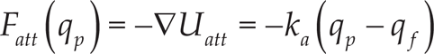
The attractive potential function is described by (2),

where qp represents the robot position vector in a workspace of two dimensions qp = [x,y] T . The vector qf represents the point of the goal position and ka is a positive scalar-constant that represents the proportional gain of the function. The expression (| qp − qf |) is the distance da existing between the robot position and the target position; in other words, the length of the line segment connecting them to obtain the Euclidean distance, which is a position function.
The attractive force Fatt(qp) is obtained by the negative gradient of the attractive potential function, as is described by (3),
The repulsive potential function has a limited range of influence; this prevents the movement of the robot from being affected by a distant obstacle. The repulsive potential function is described in (4), and was given by Khatib [2].

where ρ0 represents the limit distance of influence of the potential field, and ρ is the shortest distance to the obstacle; the constant kr is the repulsive proportional gain.
The repulsive force Frep(qp) described in (5) keeps the robot away from the obstacles, hence its name: Force Inducing an Artificial Repulsion from the Surface (FIRAS, from French) [2],

where
The APF is widely used in path planning for mobile robots because of its simplicity, mathematical elegance and effectiveness in providing smooth and safe planning; unfortunately, it has limitations in many real-world applications where the environment is dynamic, and therefore classical APF becomes impractical, producing inefficient path planning [20]. For the above reasons, the APF method is complemented by various techniques with the aim of mitigating or avoiding these limitations. In particular, this paper presents a novel and flexible algorithm based on the PBGA to obtain the optimal values for the APF, such as step size, ka(opt), and kr(opt). The algorithm is able to work with one or several processors, which is important because nowadays there are many AMRs with a uniprocessor on-board computer system. On the other hand, new AMRs have multiprocessor on-board computer systems.
The PBPF proposal effectively combines the PBGA and the APF methods to obtain an efficient path planning method for AMRs that can provide optimal paths, whether they exist, in complex real-world sceneries. In algorithm 2, the pseudocode of the PBPF proposal is shown, where the proportional gains are evolved with the PBGA (algorithm 1); the PBGA uses as the fitness function (FitFunc) the APF method explained in algorithm 3. In particular, the prototype function of PBGA is

on the right side of the function, [var1,…,varn] are the parameters that will be optimized (ka, krN, and the step size (η)) using a specific rate of bacterial mutation, a crossover type, and a selection method (all of them contained in PBGAparam) in order to meet an optimization criterion based on the fitness function FitFunc; finally, the parameter Np is the number of processors to be used. The return values var1,…,varn are the optimized variables ka, krN, the step size (η), number of configuration (m), goal, and da, which is the AMR distance to the target and is directly related to the fitness value (fitValue).
The input parameters for the PBPF path planner are those required by the algorithms: PBGA (algorithm 1) and APF (algorithm 3). A point to consider is that the sequential implementation of PBPF is when Np (number of processors) is equal to one, otherwise the values of Np ∊ ℕ larger than one allow the parallel implementation of PBPF. In line 2 of algorithm 2, a function handler FitFunc is used to facilitate the writing of the pseudocode; this is equivalent to writing the APF fitness function including all its parameters. In line 3, the PBGA evolves the parameters ka, and krN =[kr1,…,krn] to obtain the corresponding optimal values if the destination point (goal) is reached. For example, if goal = 1, by using the value da the user can verify if the AMR has reached the destination point, given that when the goal is reached da≤ε. Otherwise, if goal =0 is returned, it means that the target point is not reached; in this case, the PBGA returns the values found, although these values are not optimal. Furthermore, the distance da is a returned value which is used to know how far the destination point is from the AMR.
Fitness function
The fitness function is based on the APF method shown in algorithm 3. It requires the next set of values: a starting position (q(0)←q0), a target position (qf), the proportional gains (ka and krN) which are the gains of attractive and repulsive potential, respectively, the position of the obstacles (ON = [O1,…,On]), the step size (η) used in the iterative calculation of the next position q (step 7), the maximal approximation error (ε) that can also be given by the user as an input to the algorithm, and the number of the maximum number of iterations M. The parameters ε and M are the algorithm stop conditions, as shown in step 4.
The algorithm starts calculating the Euclidean distance (da), to determine the distance between the AMR position and the target position. Next, the algorithm enters into a loop to move the AMR step by step. Inside the loop, the total potential field Utotal (q(m)) is calculated using equation of step 5 based on (2) and (4), where n is the number of obstacles. Step 6 consists of calculating the negative gradient of Utotal(q(m)) to obtain the generalized force F(q(m)), which is used in step 7 to iteratively calculate the new position of AMR. In step 8, the new existing distance da between the actual AMR position and the target position is calculated. The loop iterates until the stop conditions are presented, from steps 11 to 15, and the algorithm verifies whether the AMR reached the target or not. For the success case da≤ε the algorithm returns a flag goal ← 1 indicating that the AMR reached the goal, and returns the configuration set (path) q and the parameters da and m. For the failure case the target position has not been achieved, and the AMR was probably in a trap situation due to local minima, or the goal position is located very close to an obstacle presenting the GNRON problem (Goal Non-Reachable with Obstacles Nearby), one more possibility of failure can be the impossibility of the AMR to pass between two obstacles located very close i.e., narrow corridors [29].
Experiments and Results
To evaluate the PBPF proposal, we developed an experimental simulation platform with the aim of demonstrating the scalability characteristic and high-performance of the PBPF proposal. The platform has the following characteristics:
To compare the performance of the PBPF with regard to other software language and implementation, three modules were developed. One module of the platform was developed in Matlab working in sequential form, and a second one was programmed in C/C++ also working in sequential form; the third module of the platform is a parallel version programmed in C/C++. It is possible to compare the PBPF in sequential or parallel forms against the APF for off-line and on-line dynamic applications.
The software has the best of Matlab and C/C++ languages, so we have used the friendly user interface of Matlab as well as the computational advantages of programming with C/C++ through the use of the Matlab MEX-file tool. The graphic interface of the experimental simulation the PBPF platform is shown in Figure 3.

Experimental simulation PBPF platform
Five experiments were carefully selected to contrast the advantages of using the PBPF proposal against the classical APF method. The experiments are organized as follows. First, the path prediction problem is presented; this experiment shows how the PBPF proposal tackles the inherent extents of the original APF. The second experiment shows the problem when a target (goal) is close to an obstacle. The third experiment regards the local minima problem, which is the most common problem in APF. These first three problems illustrate the inherent limitations of the original APF method, and have been documented in [30, 19, 31, 32, 20, 27], based on mathematical analysis, and in [31, 33, 6]. The fourth experiment is a special case to demonstrate the collision avoidance capability of the PBPF method; the collision problem occurs when the proportional gains are not well selected in the APF method. In the fifth experiment, the feature to work on-line in unknown environments of the PBPF proposal is tested.
To achieve the comparisons between the PBPF proposal and the classical APF method, we used the next criteria. For the PBPF path planner we have:
The AMR model is given by qp = (c,r,θ); which means that it has a physical size representation given by its radius r = 0.175 with the centre at the point c = (x,y), and its orientation is given by θ. To avoid wrong comparisons, in all cases we have considered that the robot is oriented to the first point to visit. Algorithms 2 and 3 allow the use of different values for repulsive gains kr's; however, the common practice in the classical APF is to use only one value of kr for all obstacles to reduce problem complexity at the decision time, and hence to make fair comparisons we have also used just one kr value for testing the PBPF method as well as its parallel version. All the experiments were achieved on a computer with the Intel Core i7–4770, which is a fast quad core processor, and it offers hyperthreading to handle eight threads at once. The base clock speed is 3.40 GHz, but due to Turbo Boost it can reach 3.90 GHz. The parameters of the PBGA algorithm are the same in all the experiments for consistency between them, so we used:
The population size consists of 16 chromosomes (individuals); each individual contains the gain parameters ka and kr, and the step size; each parameter is codified using eight bits. The gain parameters are constrained, so ka and kr≤49. Single point crossover is used, and a random point in two chromosomes (parents) is chosen. Offspring are formed by joining the genetic material to the right of the crossover point of one parent with the genetic material to the left of the cross over point of the other parent. The elitist selection method was used, and the selection rate of 0.5 (50%) performed adequately. For the APF and PBPF methods we set M = 2,500 to indicate the maximum number of steps (robot configuration position) allowed. The convergence radius ε was set to 0.175. In all the experiments, the execution time refers to the time required to find and optimize the resulting path.
Considering that 'trajectory planning and following' is a complementary task of path planning, and is not part of this work, some particular considerations to illustrate the proposal were made. They are:
The path planner experimental platform considers an AMR qp = (c,r,θ) that will follow the optimal path found by the PBPF point to point. It is supposed that the obtained trajectory plan for our AMR will couple perfectly with the optimal positions obtained by the path planner. Because it is important in path following (navigation) to consider the required time that the robot lasts to go from one position to another one, in order to make fair comparisons the following assumptions were made:
The time to orientate at each position is constant. The AMR navigation speed is constant. The time to get the next point depends on the distance.
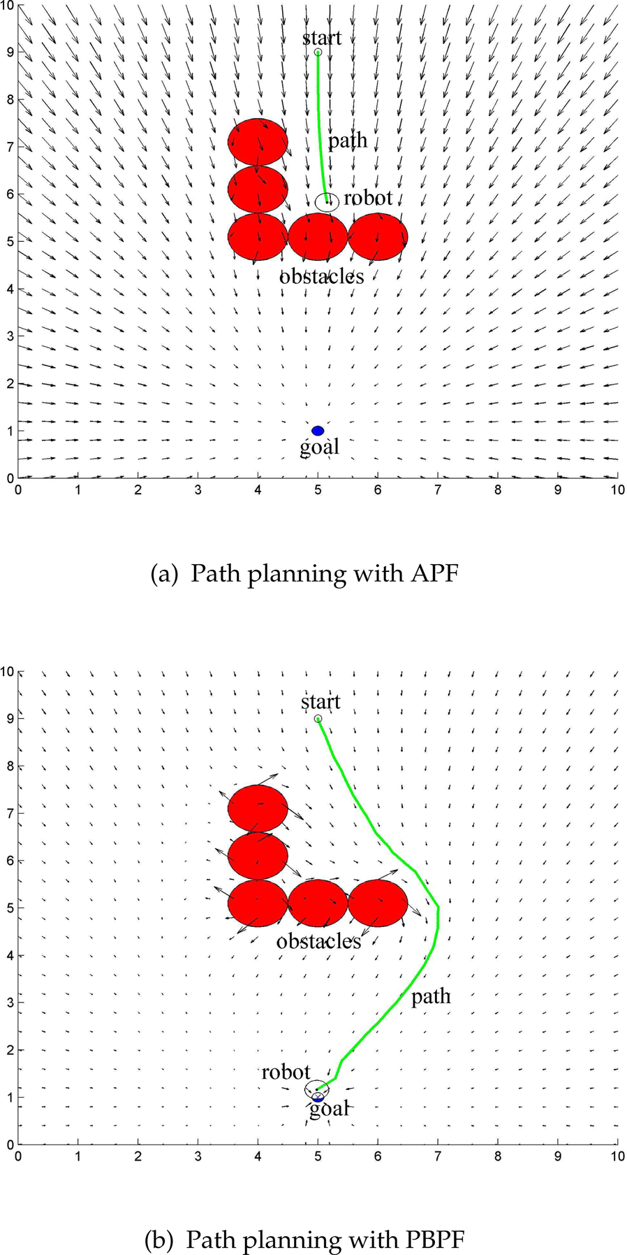
A disadvantage of the APF is the difficulty in predicting the path when the APF is not provided with the right proportional gains. In [30, 27], some examples with complex environments making path planning difficult for the APF are presented. In practice, the proportional gains of attractive and repulsive potential functions must be carefully chosen to ensure the avoidance of obstacles, since oscillation sometimes occurs in the presence of obstacles [6]. In addition to the above, the paths generated are usually far from the optimum, or in the best case are inefficient, as shown in Figure 4(a).

Experiment 1: Path prediction problem
The conditions of this experiment are: the starting point is at (5.00, 9.00), the target point is at (5.00, 1.00), and five obstacles with a radius of 0.50 and centre position are at (4.00, 6.50), (2.50, 6.50), (5.00, 3.50), (6.50, 3.50), and (8.00, 3.50). In Figure 4(a) the path prediction problem exposed by this experiment can be seen graphically, in which the AMR stopped at point (3.81, 0.00) when it should have reached the destination point (5.00, 1.00). Figure 4(b) shows the right path planned, obtained with the PBPF proposal. The time to obtain the appropriate proportional gains to solve the path prediction problem is shown in Table 1. A comparison between different platforms of implementation, and a summary of the results for the navigation simulation for this experiment, are presented in Table 2.
Experiment 1 – Execution time for different platforms

Experiment 1 – Summary of results using the APF and the PBPF proposal

When working in sequential mode, a great advantage of programming the PBPF method in the C/C++ can be observed; the computation only lasts 3.95 seconds, contrasting with the Matlab platform that last 8.98 seconds, as is shown in Table 1. On the other hand, in parallel mode (parallel execution of the algorithm using the CPU cores) the computation lasts 1.11 seconds to find and optimize the resulting values. The parallel version of the PBPF outperforms the sequential version approximately by a factor of 3.56 (i.e., 255%); this computation time for path planning is very appealing for real-world applications.
Figure 4(a) shows a wrong path achieved by the APF; here, heuristic proportional gains (ka = 2.00 and kr = 45.00) were used. In this experiment with APF, path planning was incorrect because the path does not lead the AMR to its target point, and the robot stops at point (3.81, 0.00) when it leaves the workspace. The AMR navigates 12.60 units off the workspace, and a set of 2281 configurations was needed without finding the target point. Quantifying the error of this experiment, we found that the AMR was located 1.6 units from the target point; this situation is unsatisfactory b because in this work the design requirements consider a maximum error of 0.175 units.
Figure 4(b) shows an optimal path calculated by the PBPF proposal. Path planning was made with the optimal proportional gains (ka = 11.16 and kr = 35.44). This path meets the objectives of an efficient and secure navigation to reach the target point. The path is efficient because the AMR navigates 8.69 units, and a set of 734 configurations to reach the target point (5.00, 1.17) were necessary; the AMR stopped 0.174 units from the target, which fulfils the design requirements.
A problem with most potential field-based methods was identified by Ge, Cui, Volpe, and Khosla, which consists of goals (destination points) non-reachable with obstacles nearby (GNRON) [34, 35, 36].
In this experiment we have the following conditions: start point at (5.00, 9.00), target point at (5.00, 4.00), three obstacles with radius of 0.30 each, and centre position at (5.00, 5.00), (4.00, 5.00), and (6.00, 5.00) respectively. Figure 5(a) illustrates the GNRON problem using the above values. In this experiment the AMR was stopped at point (5.19, 6.63), because if the robot continues with the movement it will be spinning around obstacles without ever being able to reach the target point at (5.00, 4.00), due to a repulsion field caused by the obstacles nearby.

Experiment 2: Goals non-reachable problem
The wrong path planning obtained with the APF method is shown in Figure 5(a); the heuristic proportional gains that were used are (ka = 2.00 y kr = 25.00). In this example, the path planning is incorrect because it does not lead the mobile robot to its target; the robot stops at the point (5.19, 6.63) because it exceeded the maximum number of iterations allowed to reach the target point. The results of this experiment are shown in Table 4; the AMR navigated through 16.35 units, and needed a set of 2500 configurations without finding the target point. The approximation error was 2.64 units, which is out of the range allowed in this work.
Similarly to the APF case, with the PBPF the AMR must navigate from the start to the goal position. Considering that one of the main problems in APF is the GNRON problem, which happens as the direction of the sum of the repulsive forces points increases and the attractive force decreases, this situation can be solved successfully by the PBPF proposal. In Table 4 the results are shown. Figure 5(b) illustrates the optimal path that allows the AMR to reach the target after 623 steps (configuration set) of the AMR. Table 3 shows the execution time of experiment 2 with the PBPF proposal, consistently to the aforementioned example; the parallel version of the PBPF outperforms the sequential version by a factor of 4.05 (i.e., 305%) since the former takes 12.72 seconds to find the optimal gain values (kr = 15.49, ka = 2.31), whereas parallel PBPF lasts only 3.14 seconds.
Experiment 2 – Execution time for different platforms

Experiment 2 – Summary of results using the APF and PBPF proposal
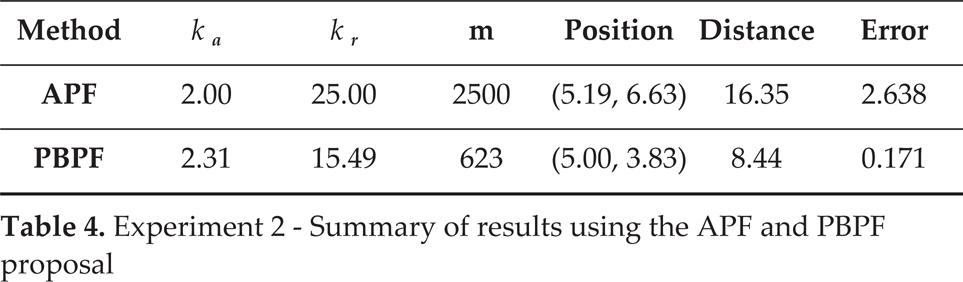
Figure 6(a) shows the case of having a local minima trap, regardless of the fact t that a valid path to the goal might exist. For this experiment, the parameters are: start position at (5.00, 8.00), goal position at (5.00, 2.00), and two overlapped obstacles with radius of 0.9 and centre at (4.25, 5.00), and (5.75, 5.00).

Experiment 3: local minima problem
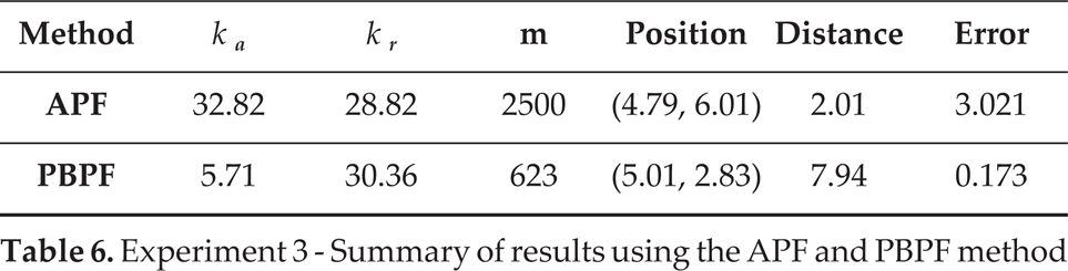
In the APF case, the user sets the gain parameters ka and kr using heuristic knowledge; however, to obtain a valid successful path, it is necessary to provide the adequate combination of gains, being common to give unappropriated values, falling in local minima traps. This is the best known situation and most cited problematic situation in APF [6, 31, 27]. Local minima can be caused by either one obstacle or a combination of them. Figure 6(a) illustrates this case well; here, the classical APF method was used to obtain the path for AMR navigation. In this experiment the AMR did not reach the target, although the algorithm iterated for an M value equal to 2500 (see line 4 of algorithm 3), which means that the AMR calculates 2500 different q positions to try to reach the target (see line 7). The results of this unsuccessful test are identified with the tag 'APF' in Table 6.
Now in the PBPF case, using the same parameters, the AMR must navigate from the start to the target position. The difference is that the gain parameters are optimized using a PBGA in the PBPF proposal. Figure 6(b) illustrates the optimal path that allows the AMR to reach the target after 623 steps (m=623) of the AMR; the PBPF results are shown in Table 6. In this case, since we are using algorithm 2 to obtain the optimal parameters, the AMR is able to reach the target fulfilling the requirement of da≤∊ it is worthwhile mentioning that the AMR used fewer steps than in the APF case. In algorithm 2 the parameter Np is equal to one, since sequential programming is used. Table 5 also shows the amount of time that the PBPF lasts to calculate the optimal gain values; hence, using sequential programming with the C/C++ platform, the algorithm lasts 4.36 seconds to find the optimal gain values. With the parallel version of the PBPF, the time that the algorithm lasts to calculate the optimal gain value is 1.15 seconds.
Experiment 3 – Execution time for different platforms

Experiment 3 – Summary of results using the APF and PBPF method
In this section, a particular case of collision avoidance is presented since it is a desirable condition to avoid for all motion planning systems. It might be tackled adequately with the APF method, as long as it has the appropriate proportional gains for the application; otherwise, it might be incurred in a path that takes the AMR to a collision in the navigation. In particular, it is known that the repulsion proportional gain is responsible for avoiding collision paths with obstacles. We present an experiment with the APF where the appropriate value of each of the proportional gains was incorrect, and collision unavoidable. To solve this scenario, the PBPF provides the adequate proportional gains to achieve the optimal path free of collisions and is capable of taking the AMR through a safe route to its destination.
The collision problem exposed by this experiment can be seen graphically in Figure 7(a). The right path that was planned with the PBPF proposal is shown in Figure 7(b). Working in the sequential mode and programming the PBPF using the C/C++ platform, the computation of the optimal path only lasts 3.35 seconds; in contrast with the above, the results obtained with the Matlab platform last 7.72 seconds, and using the CPU cores and parallel mode the computation time was 0.95 seconds, as shown in Table 7.
Experiment 4 – Execution time for different platforms
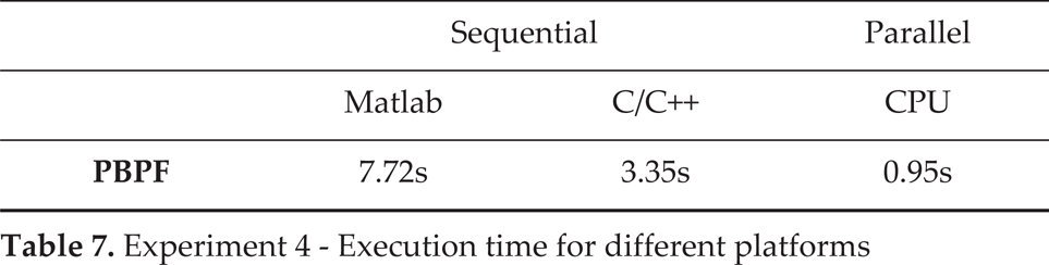
Experiment 4 – Execution time for different platforms
Experiment 4 – Summary of results using the APF and PBPF proposal

Experiment 4: Collision problem
Figure 7(a) shows a truncated path that was achieved with the APF method; the proportional gains (ka = 25.00 and kr = 10.00) were provided heuristically. The path planning was incorrect because this path did not lead the AMR to its target point; the robot stopped at point (5.15, 5.82), before a crash could occur. The robot navigated without finding the target point; 3.18 workspace units and a set of 164 configurations were needed, leaving the robot 4.288 units far from the goal; this situation is unsatisfactory and unsafe.
Figure 7(b) shows an optimal path obtained with the PBPF, the calculated proportional gains were ka = 10.60 and kr = 41.09. This path meets the objectives of an optimal and safe navigation to reach the target point. The path is optimal because it is the best; the AMR navigates 8.99 units, and a set of 654 configurations was needed to reach the target point (5.00, 1.17); the final approximation error was 0.172 workspace units, fulfilling the design requirements of this set of experiments.
An advantage of the off-line mode is that the environment is known; however, real-world applications frequently face the AMR to unknown or partially known environments, where the already planned path needs to be adjusted for reaching the goal. This operating mode is referred to as online [37].
The APF cannot work well in the on-line mode of path planning, where random positioning of obstacles as well as moving obstacles (dynamic obstacles) exist, because the APF requires that the parameters are set in the 'manual' form of operation. The existence of a non-static world configuration requires the use of the 'Automatic' form for updating the parameters.
In this experiment, we tested the PBPF method by placing an obstacle at random in such a way that it blocked the optimal path already found, interfering with the AMR previously planned path. In this case, the random obstacle remained static once it was placed.
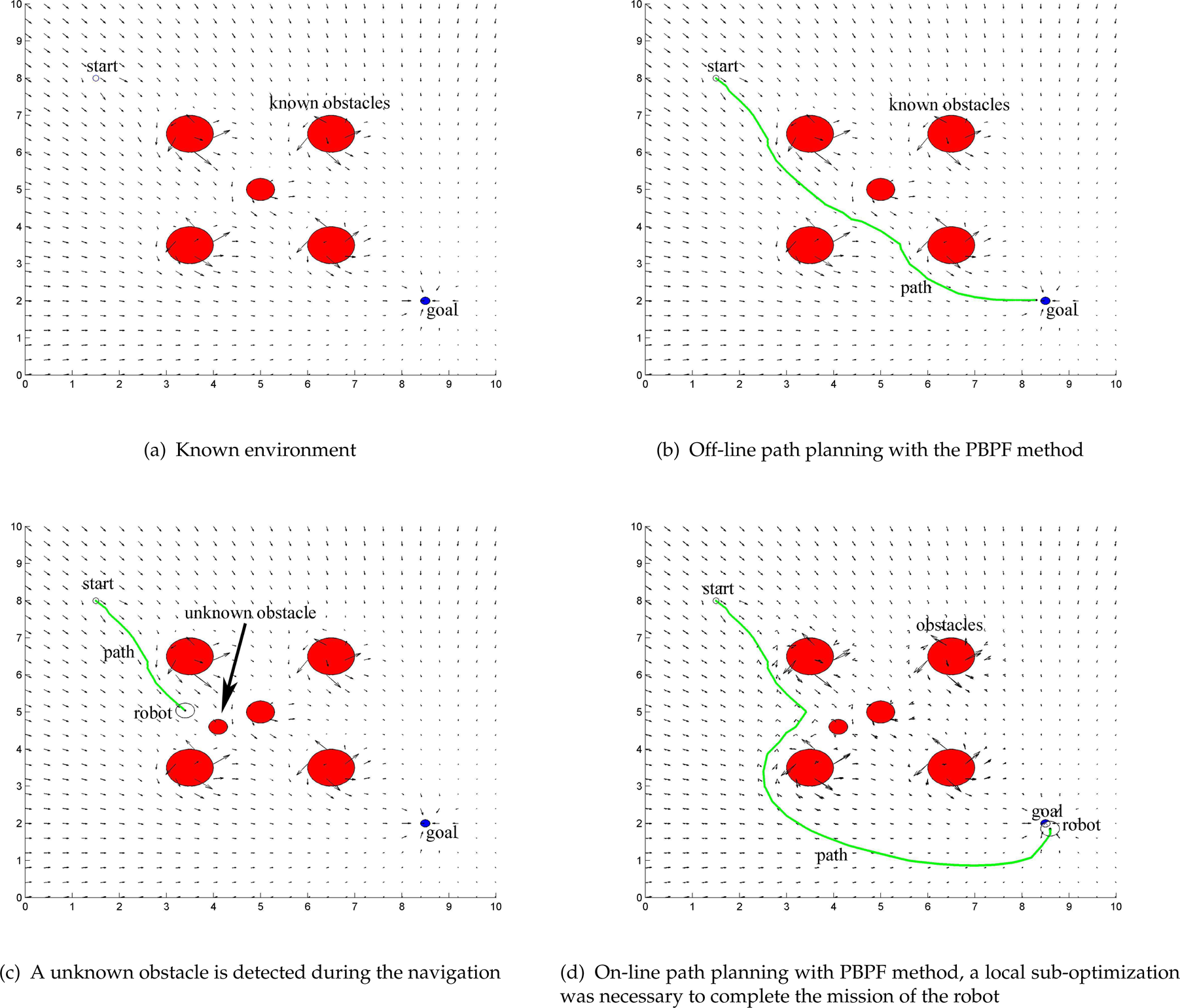
In this experiment, for the above reasons only the PBPF method was used. At the beginning of the experiment the environment was known, the start point was at (2.00, 8.00), the goal point was at (8.00, 2.00), and there were five obstacles placed at positions (5.00, 5.00), (3.50, 3.50), (3.50, 6.50), (6.50, 3.50), and (6.50, 6.50); the PBPF method was tested using the above world configuration, see Figure 8(a). The experiment was conducted as follows:
Path planning is achieved in the off-line mode because the environment is known; see Figure 8(b). We switched to the on-line mode, the navigation started, and the AMR followed the path plan showed in Figure 8(b). Afterwards, an obstacle is added at position (4.10, 4.60) to make a change in the environment (world configuration) for the AMR; see Figure 8(c). The AMR at the position (3.40, 5.04) senses the obstacle, and it calculates the obstacle position to update the world configuration. The path planner of the AMR now has a different world configuration; hence, it is necessary to update the path by recalculating the set of parameters needed by the PBPF method. The AMR follows the new path to reach the goal; see Figure 8(d).
Table 10 shows that the PBPF was capable of obtaining the optimal parameters to reach the goal in the two operating modes: off-line and on-line. However, there exists a substantial difference in the computational time to obtain the solutions; the parallel version of the PBPF outperforms the sequential version of the PBPF approximately by a factor of 3.6 (i.e., ≈ 260%) in both cases, see Table 9. Therefore, the parallel version of the PBPF is the most suitable for on-line applications.
Experiment 5: On-line path planning for unknown environments
Experiment 5 – Execution time for different platforms for the PBPF1 in off-line mode, and for the PBPF2 in on-line mode

Experiment 5 – Summary of results using the PBPF1 in off-line mode, and the PBPF2 in on-line mode

A path planning proposal, the PBPF method, for off-line and on-line applications with unknown obstacles was presented. Simulation results demonstrate the effectiveness of the PBPF proposal in contrast with the APF method. The PBPF path planning method for AMR navigation is based on the traditional potential field approach enhanced with the pseudo-bacterial genetic algorithm to tune the parameters. It provides a feasible, safe, and optimal path for real-world complex environments. The PBPF method uses evolutionary computation to provide a reachable set of optimal configurations qopt = [q0,q1,…,qf] ∊ ℝn, which are the positions of the AMR that connect the starting position q0 to the final position qf. This is in contrast to the APF method, which does not guarantee finding a reachable set even though it may exist.
A simulation platform using a mobile robot model with physical size in the plane, position, and orientation was used to achieve the experiments. The results show that the APF can fail in scenarios where a reachable configuration set exists because the proportional gains are mainly based on heuristics. Additionally, the APF did not work well with dynamic scenarios because the APF uses fix gains, and dynamic scenarios require us to recalculate the gains to adjust the AMR to the new situation. The PBPF proposal method worked adequately in all experiments; however, the parallel version of the PBPF method outperforms the sequential version in finding the optimal paths. The parallel version of the PBPF method provides lower computation times, making the method suitable for on-line applications in complex real-world scenarios for complex missions, where dynamic environments with obstacles changing its position may exist, and to recalculate the optimal path (configuration set) is mandatory.
The PBPF method can be used in sequential mode for low-cost on-board computers, or in parallel mode, to take advantage of novel computing architectures that provide more than one CPU in the same board. The parallel mode might be critical, since although the AMR may have efficient machines on-line path planning is a complex task that might require most of the CPU time. Hence, by using multiple CPUs units, the AMR will be able to achieve other important tasks such as trajectory planning and following, sensing, and other navigation functions.