Large and Dense Swarms: Simulation of a Shortest Path Alarm Propagation

Abstract

This paper deals with the transmission of alarm messages in large and dense underwater swarms of Autonomous Underwater Vehicles (AUVs) and describes the verification process of the derived algorithm results by means of two simulation tools realized by the authors. A collision-free communication protocol has been developed, tailored to a case where a single AUV needs to send a message to a specific subset of swarm members regarding a perceived danger. The protocol includes a handshaking procedure that creates a silence region before the transmission of the message obtained through specific acoustic tones out of the normal transmission frequencies or through optical signals. This region will include all members of the swarm involved in the alarm message and their neighbours, preventing collisions between them. The AUV sending messages to a target area computes a delay function on appropriate arcs and runs a Dijkstra-like algorithm obtaining a multicast tree. After an explanation of the whole building of this collision-free multicast tree, a simulation has been carried out assuming different scenarios relevant to swarm density, signal power of the modem and the geometrical configuration of the nodes.

1. Introduction

The communication of robotic swarms and the consequent behaviour of the system [1], its stability [2, 3] and the capability of making shared decisions to pursue an established mission [4, 5, 6] are a well-consolidated field of investigation in modern robotics. Less debated are some classes of problems that can happen in difficult and peculiar environments, such as underwater and space. In particular, the propagation of alarms or other important actions needed in underwater swarms must usually deal with important protocol exceptions [7, 8], suspending the normal management of communication [9, 10] to speed up the alarm transmission times as much as possible. The scenario that we considered is based on a different case that represents the final target of our research: the realization of a dense mobile network characterized by a short range (typically 3–10 m. of internodal distance), multihop and high-speed communication capabilities.

In our work we have proven that this kind of network can be physically realized, maintaining the cost of the whole system compatible with practical applications. The use of a large number of very low cost vessels can have significant advantages for the few, far more sophisticated and expensive vehicles that serve as the current market reference in all of the cases where the monitoring/surveillance of a wide area in short times is the main target of the mission, and when a significant interaction between surface and submerged agents is important. In fact, apart from the advantages and disadvantages relevant to specific functionalities, one of the most important issues is that the availability of a high-speed communication network, distributed in a large volume, can allow real-time communication with the multibody system and therefore direct control 'during' the mission.

Such a kind of mobile network can exhibit significant problems when absolute priority messages must be sent to distant areas of the network. The reasons for this are mostly relevant to the limitations of the physical channel that imply very long times for each hop because of the high competition caused by the 'swarm' networking operation.

This study, carried out with the purpose of coping with this specific problem, is part of a larger research activity started within the 'Harness' project, funded by the Italian Institute of Technology (IIT), and which has the objective of defining how far and at which length of time information can arrive in a large, multihop network to still allow a real-time response. We called this locus the 'knowledge horizon'.

In the paper we will not discuss the knowledge horizon problem (see a preliminary discussion in [11]) but we will focus on alarm transmission. This often represents a tradeoff between the mission success and the failure of the system, so an efficient solution has been proven to be mandatory. To this aim we took advantage of other software tools developed within Harness, such as simulation software, based on the open source 'GAZEBO' framework [12] that allows us to visualize and measure the physical behaviour of a swarm under realistic conditions. Moreover, in the current work we also exploited the results given by the Harness network simulator, based on the OMNET framework simulation machine.

We intend to present how the choices carried out within the research job led to credible results giving numerical information in terms of propagation times of the alarm messages. A physical demonstration of these algorithms is expected over a year from now, in a project currently under preparation that aims at security purposes and which will see the operation of a swarm larger than ten vessels.

We give a short outline of the paper: in section 2 we present a static network model of the problem, in section 3 we describe in detail the physical layer of our underwater communication network, in section 4 we present our alarm spreading collision-free protocol, in section 5 we give details of the delay function that we use in the arcs of our model's network, finally in section 6 we present the simulation results, and in section 7 we sum up with conclusions and next steps.

2. Modelling the Problem

Suppose that an AUV perceives a threat for a target subset of the swarm that is far from it (i.e. it cannot directly send a message to all members of the subset avoiding forwarding). Clearly this AUV, which we will call the source (denoted with 's'), has to send an alarm message to the subset in such a way that:

The message arrives to all members of the target set.

The message arrives as fast as possible to all members of the target set.

We also assume that the message is sent through an acoustic channel. Requirement 1, in our experience, usually implies the need for a deterministic communication protocol (and in particular a deterministic medium access control (MAC) protocol). We underline that in most practical cases deterministic MAC protocols in the framework of large underwater swarms of AUVs are not a good solution if associated with every kind of message, mostly for the long delay introduced by approaches like TDMA (Time Division Multiple Access) or the technical challenges introduced by CDMA (Code Division Multiple Access) approaches with narrow bandwidth and Doppler effect [13].

In what follows we are going to propose a model to tackle requirement 2. Firstly, we need to specify the assumptions under which we develop our model. We will assume that we can treat our set of embodied agents and the communication network between them as a static network. However, the mobility of the AUVs (and their specific dynamics) is considered when a node perceiving a threat has to determine a subset of nodes that will be affected by the threat.

Every agent is identified with a node of the network, and two nodes, u and v, are connected by a directed edge uv, or more simply an arc uv, if u can communicate with v. In order to maintain maximal flexibility we maintain directions, because it may be possible that u can communicate with v but v cannot communicate with u.

The assumption of a static network is justified by the fact that in dense networks of AUVs the mobility of the agents is not very relevant with respect to the transmission speed (time of flight, duration of the data transmission) in the selected channel.

Finally, we assume that each node of the network knows the positions of all of the other members of the swarm, the approximate amount of delay (introduced by noisy transmission of data, by the MAC protocol and by the chosen modulation scheme), the average number of retransmissions required for a packet of length L, and the capacity (i.e. the bit-rate) available on each connection of the network.

Given all the assumptions, we reasonably suppose that the source (and every other node) can associate to each arc e of the network a delay function τ(e). Moreover, each arc of the network has an associated capacity (or bit-rate), that we denote with c(e). Let us indicate with P=(v₀, a₁,v₁, …, a_k,v_k), with k≥0v₀, v₁, …, v_k∊V and distinct and a₁, …, a_k, ∊A, a directed path as defined in [14]: we associate with P its delay and its capacity $\text{τ}\left(\mathrm{P}\right)={\displaystyle \sum }_{\mathrm{e}\in \mathrm{P}}\text{τ}\left(\mathrm{e}\right)$ , $\mathrm{C}\left(\mathrm{P}\right)=\underset{\mathrm{e}\in \mathrm{P}}{\min }\mathrm{c}(\mathrm{e})$ . We observe that given a path P from a source to a member of the target set v the time necessary for a packet of length L to reach the destination can be expressed as τ(P) + L/C(P), where the second term C(P) accounts for direct transmission. Hence, in order to satisfy requirement 2, we may simply find a path P from s to v that minimizes τ(P) + L/C(P). This problem is known as finding the quickest path from s to v and was introduced by Chen and Chin in 1990 [15].

The problem is polinomially solvable in time O(|A|² + |A| |N| log |A| |N|) where A is the set of arcs of the network we are considering in the algorithm and N is the set of nodes) [15, 16] when we fix the packet length L, and the algorithm requires the transformation of the original network in an auxiliary network without capacities where Dijkstra's algorithm [17] is run. The quickest path problem was also analysed by Chen and Hung in 1993, where they solved the problem for every pair of vertices in the graph in time O (|A| |N|²) [18, 19], without requiring any graph transformation. We observe that even if one would like to solve the problem from a single source to multiple sinks, in the worst case he needs the same computations performed by the algorithm of Chen and Hung for the all pairs problem.

As Chen and Chin interestingly observe, the term L/C(P) prevents us from using a Dijkstra-like algorithm because it does not hold true that 'parts of a quickest path are quickest paths'. In particular, this means that when we find a set of paths from a source to multiple destinations, in general this set cannot be reduced to a tree, as happens for the shortest paths.

In a first approach, for the sake of simplicity we assume that every arc e has the same bit-rate or capacity that we denote with C. This assumption can be realistic when the packet length L is small compared to the bit-rate of every arc, and also in every practical framework where the only reliable bit-rate information is the peak bit-rate (which is uniform in a network where every AUV has the same modem).

In this case we want to minimize τ(P) + L/C where L/C is a constant, that is we can find a shortest path (in terms of delays) from s to v. As all the transit times are nonnegative, we can use for shortest path computation the algorithm of Dijkstra. Doing this for every source-destination pair, we end up finding a shortest path tree via Dijkstra's algorithm, where s is the root, and the set of nodes considered could be the entire network or a subset of it, selected by the source through its sensing of the threat.

We finally recall some basics about Dijkstra's algorithm. First of all, in this case we can use it because our weight function is nonnegative. Dijkstra's algorithm visits the vertices of a network according to a potential function built during its execution. This potential function is associated to every node, and at the beginning of the algorithm is 0 for the source and a very high value (ideally infinity) for every other node. At run time, the potential function associated with a node represents the currently shortest time to reach that node. At the end of Dijkstra execution, when every node has been visited, the potential function of a node v, which we will further indicate with p(v), will represent the shortest time to reach v with the alarm message.

3. Physical Layer Communication

In section 2 we have described a simple model for the quickest delivery problem. In order to give appropriate weights to the edges, and in order to treat the problem deterministically, we have to describe a physical layer technology and tailor a specific MAC and routing protocol in the same framework. In this section we describe the physical layer communication protocol that relies on the technological solutions developed in the framework of the IIT-financed Harness project.

The mobile network is a swarm of underwater robot-nodes that uses exchange of data and control information for working as a single multi-body agent. Underwater Wireless Sensor Networks (U-WSN) have different factors influencing performance requirements [20] with respect to terrestrial ones. Therefore, key challenges in underwater communications are needed and give motivations for different choices in the architecture protocol and algorithm design. For physical layer technology, as in [8], a system based on an underwater acoustic modem is considered. With respect to a traditional underwater wireless sensor network and to usual AUV teams, in a dense swarm network, like that which our group is developing, the distance between robots can be very short, ranging from a minimum secure distance of 3m to a maximum of several tens of metres. In these conditions it is possible to achieve a greater bandwidth, as shown in [9], where, to obtain a good tradeoff between bandwidth and efficiency, an isotropic transducer operating at hundreds of kHz was considered. This value for signal frequency is higher than those used in traditional underwater acoustic networks, with an increase in bandwidth and less harmful multipath effects. The network typically works in coastal or shallow water, where the multipath effect is stronger. The modulation format adopted for an acoustic shallow water channel is M-Frequency Shift Keying (M-FSK), which is more prone to contrasting the multipath effects and allows the design and realization of a low-cost modem. The communication modem used is designed for the M-FSK signal, and the modulation parameters can be set in terms of number of frequency used, symbol time duration, time guard duration, transmission power and other settings. In this primary version, the acoustic modem does not allow an adaptive modulation, but after simulations and previous measures in the working environment the modem parameters can be set and remain constant for all nodes in the network. This modem represents a suitable tool for communications testing in these peculiar conditions, and allows the off-line setting of communications parameters. The acoustic channel has been assumed as affected by Rayleigh fading (RFC, Rayleigh Fading Channel). Thus, the error probability per symbol, P_M, can be expressed as [21, 22]:

$${\mathrm{P}}_{\mathrm{M}}={\displaystyle \sum }_{\mathrm{n}=1}^{\mathrm{M}-1}\left(\begin{array}{c}\mathrm{M}-1\\ \mathrm{n}\end{array}\right)\frac{1}{1+\mathrm{n}+\text{nk}\cdot \text{SNR}}$$

(1)

where M is the levels number, k the bits per symbol, SNR the signal-to-noise ratio, related to the ratio E_b/N₀ (where E _b is energy-per-bit and N₀ is the noise power spectral density) by:

$$\frac{{\mathrm{E}}_{\mathrm{b}}}{{\mathrm{N}}_0}=\text{SNR}\cdot \frac{\text{BW}}{\text{BR}}$$

(2)

where BW is the bandwidth and BR is the bit-rate. The bit-rate depends on the modulation format adopted and symbol time associated as a:

$$\text{BR}=\frac{{\mathrm{N}}_{\mathrm{C}}\cdot {\text{log}}_2\left(\mathrm{M}\right)}{{\mathrm{T}}_{\mathrm{S}}+{\mathrm{T}}_{\mathrm{g}}}$$

(3)

where T_S is the symbol time duration, T_g is the time guard used for reducing the multipath effect, N_C is the number of carriers used simultaneously. Symbol time duration can be set by modem but depends on frequency space, in order to ensure the orthogonality between the carriers. Time guard duration allows us to reduce the multipath effect that depends on the acoustical channel parameters; an increase in the time guard obviously reduces the communication capacity.

We would like to point out that the SNR adopted in the simulation results presented in this paper has been derived by standard noise level generally accepted for coastal environments. These values are subjected to considerable variations, depending on the specific area considered, the relevant wave features, the noise generated by human activities, streams, temperatures and many other factors, but we assume that for most of the practical conditions they represent a reasonable approximation.

What is still lacking is the portion of SNR relevant to possible multipath disturbances generated by the reflections on the same AUV-nodes of the swarm. According to preliminary calculations, the AUV-nodes have been modelled as simple cylinders of about 160mm in diameter. Thus, the power that is backscattered should be negligible in terms of the contribution to the SNR adopted into the algorithm (1–3). Nevertheless, this assumption must be proven for the final vessels. In fact, the continuous improvement of the first very basic vessels adopted in the Harness project caused the introduction of several scattering areas/volumes with convex shapes and the possible generation of strong reflected waves along specific directions.

Additional investigations and tests have been planned to validate current assumptions or to modify the SNR value accordingly in the algorithm that gives the BR value. As far as this concerns the aims of the current paper, the values adopted hereinafter are suitable starting points for the original AUV vessels.

4. Building a Collision-free Multicast Tree

In this section we describe how we can aim at the fast delivery of an alarm message on a large underwater swarm relying on the model described in section 2. We remind here that we want to build a collision-free protocol because, in a slow channel, collision and retransmission modes are time consuming and impractical.

4.1 Signalling Procedure

When an underwater swarm of vessels is in a normal cruising mode, all members exchange each other various kinds of messages, mostly on their positions, velocities and data from internal and external sensors, but also commands and long sensing datasets. When an external threat is perceived by the source, the first thing the source should do is to silence its first and second neighbourhoods in order to avoid collisions with its neighbours.

In this paper we describe a simple signalling procedure that aims at creating a silence area around the transmitter(s). The main feature of this procedure is that it has to be performed on a different channel than that used to transmit messages, it does not interfere with messages transmission and reception, and two signalling messages do not collide each other (i.e. who receives can still distinguish that it has received a signalling message of a certain type). As an example we can think of optical signals, i.e. 'coloured' light flashes generated by suitable LEDs. Two different signalling signals will have two different colours. Note that colour is simply a practical scheme to think about: we could use two different flash sequences or more suitable markers. Note also that light signals can only be adopted in 'dense' swarms; in less strict distance requirements only low frequency pure acoustical tones could be adopted. Optical transmission in a 'dense' swarm network is currently constrained by several limits. The signal must be emitted with a radiation pattern covering an almost 4τ solid angle (so laser sources are therefore generally inadequate), the source and the relevant electronics must be cheap because of the large number of nodes, and the source has to be very intense to cover a distance range comparable to the acoustical one which is also not in perfectly clean waters. Note that in any case a fully functional acoustical network must be available, to cope with the case of dirty water, which is a very common situation close to the coasts. We are working on this, and the technology is in a very fast advancement phase, but currently the most practical sources are high power and high efficiency LEDs, and their modulation capability is limited to short OOK (On Off Keying) modulation in order to achieve the maximum light intensity and fit with all of the above-mentioned requirements.

We start describing the procedure for the source:

s sends a first Ready To Send (RTS) signal and waits an appropriate time before starting the transmission of the alarm message.

All neighbours of s receiving the RTS will not start transmission of new messages (but they finish their ongoing transmissions if present).

All neighbours of s receiving the RTS send a Clear To Send (CTS) signal after finishing any ongoing transmission.

Upon reception of the CTS signal, the second neighbourhood of s acts like the neighbours of s in step 2.

In step 1 the source indicates that it has the need to start transmission of the alarm message, and warns its neighbours. In step 2 the neighbours of s silence themselves in order to properly receive the alarm message, and in step 3 they warn their neighbours in order to avoid collisions upon multiple reception. In step 4 the second neighbourhood of s silences upon reception of the CTS signal in order to avoid collision for multiple reception at the first neighbourhood of s.

A final note about how much s has to wait: suppose the maximum packet length admitted on the network is P₁, then s has to wait:

$$2\tau +2{\mathrm{d}}_{\text{max}}^1/\mathrm{c}+2{\mathrm{d}}_{\text{max}}^2/\mathrm{c}+2{\mathrm{P}}_1/\text{BR}$$

where τ is the transmission time of the RTS and CTS signal, ${\mathrm{d}}_{\text{max}}^1$ and ${\mathrm{d}}_{\text{max}}^2$ are the distance between s and the most far first neighbour and s and the most far second neighbour respectively, c is the speed of sound in water and BR is the bit-rate.

For what concerns the first neighbourhood of s, every node has to wait until it receives the alarm message, whilst the second neighbourhood has to wait until it receives a new RTS signal or a timeout.

Once s has completed this signalling procedure, it sends the alarm message, which will not collide with any other message due to the signalling procedure. The neighbours of s that are in the shortest path tree (which is sent together with the alarm message) have to forward the message. Before doing this, each of them starts the signalling procedure, with the only difference being that they have to wait before transmitting the alarm message for a shorter time, because their neighbours are already silent due to step 4. In particular, they have to wait a time:

$$2\tau +{\mathrm{d}}_{\text{max}}^1/\mathrm{c}+2{\mathrm{d}}_{\text{max}}^2/\mathrm{c}+{\mathrm{P}}_1/\text{BR}$$

4.2 Communication Protocol

Suppose s has to send an alarm message to a target area. The steps it must perform are:

Select an appropriate region where the message must go in order to arrive at the target area (mainly using simple geometrical criteria).

Using the last available data and the number of AUV in the selected region, compute the length of the alarm message and the delay function on the edges of the network; the delay function will include the time spent by each node running the signalling procedure.

Run a Dijkstra-like algorithm on the network.

Append the computed shortest path tree and the potentials of each node to the alarm message; this step is crucial for 'smart forwarding'.

Start the signalling procedure.

Send the message.

Next we must specify the protocol rules for every other node different to s in the region selected by s. In the following we will indicate with leaf a node of the tree that has indegree 1 and outdegree 0 (alternatively there is only an arc uv entering in the leaf v). In other words, a leaf should be a node in the target set that does not have to further forward the alarm message. When we say that two nodes are at the same level of the tree, it means that they have the same distance in the tree from the source s in terms of number of hops. Finally, we will indicate with $\mathrm{p}:\mathrm{N}\to {ℝ}^{+}$ the output potential function from the Dijkstra-like algorithm.

The base protocol rule describes what should be the behaviour of a node v receiving an alarm message:

If v does not have any neighbour at the same level in the tree then it must forward the alarm message.

If there exists a node u in the same level of the tree and p(v)>p(u), then v has to wait for u to transmit (i.e. it has to wait the time that waits u and the transmission and propagation time of u). The procedure has to be made for every other neighbour of u with p(v)>p(u) in an ordered way (from smaller to bigger potential).

If v has a neighbour at the same level, say u, and p(v)<p(u), and this holds for all the other neighbours at the same level if any other, then v must immediately forward the alarm message.

If v has a neighbour at the same level, say u, and p(v) = p(u), then the node with a smaller third position coordinate will transmit first; the other will wait an appropriate time (see next subsection).

Every node forwarding an alarm message must start the signalling procedure and indicate itself as the source of the message it is sending.

From the signalling procedure we obtain collision avoidance for each node with respect to its predecessor and successors (both at the transmitter and at the receiver). Nevertheless, with this rule only, collision could still be possible for nodes at the same level of the tree. In order to avoid this, we have designed rules 1, 2 and 3 that describe what we call a turnation rule. In next subsection we explain in detail how this rule must be correctly integrated inside the Dijkstra-like algorithm. Finally, rule 4 is simply a parity-breaking rule; any other parity-breaking rule could be implemented.

4.3 Turnation Rule

We recall that the algorithm of Dijkstra selects the next node to visit as that with the smallest potential. This means that, if we fix a level of the network section determined by source s, the first node that will receive the alarm message is exactly the first node of that level selected by Dijkstra's algorithm.

We can exploit this property in the following way. First, we append our network from s, and we run a Breadth-First Search (BFS); in this way we know the distance for each node from s, i.e. its level. When a node v is visited during Dijkstra's algorithm, we check if there are any neighbours and second neighbours of v, at the same level of the tree of v, that have already been visited; if this is the case we modify the weight of all the edges going out from v. The rationale behind this is that v has to wait for all nodes to transmit, and we include this waiting time in the weight function on the edges.

Let us indicate with t_w(v) the delay introduced by the transmission of the node v:

$${\mathrm{t}}_{\mathrm{w}}\left(\mathrm{v}\right)=\raisebox{1ex}{${\mathrm{d}}_{\text{max}}\left(\mathrm{v}\right)$}\!\left/ \!\raisebox{-1ex}{$\mathrm{c}$}\right.+\raisebox{1ex}{$\mathrm{A}$}\!\left/ \!\raisebox{-1ex}{$\text{BR}$}\right.+\delta$$

where d_max(v) is the distance between v and its furthest second neighbour at its level, A is the length in terms of bits of the alarm message, while δ is a small quantity of choice. We visit the nodes of a level from the smallest to the biggest potential. To the arcs going out from the node we are visiting, we add the waiting time already assigned to the first and second neighbours already visited and t_w(v) (avoiding repetitions). Finally, when the tree is built, we remove from the delay assigned to nodes in the tree the delays ${{\displaystyle \sum }}^{\text{}}{\mathrm{t}}_{\mathrm{w}}(\mathrm{v})$ of the nodes v outside the tree.

The standard Dijkstra's algorithm visits each node once, but in our approach we propose changing the edge weights during execution so that we need to perform a small amount of pre-processing after the BFS. In particular, we remove all edges going back to source s; that is, we remove for every 2≤k≤K, all the edges going from level k to level k−1. We underline that this procedure could delete some paths, but reasonably these paths are not interesting as they do not promote the forward propagation of the alarm.

Finally, we observe that this weight augmenting procedure is coherent with rules 1, 2, 3 and 4 (as the parity must be broken in the same way).

4.4 Pruning

After the running of the Dijkstra-like algorithm, we obtain a tree that includes all of the nodes selected at the beginning by s. If some of the leaves of this tree are not included in the target area, we may delete them from the tree and iterate this procedure until all the leaves of the tree are in the target area. This pruning could be effective if, for example, s makes a very rough selection of the area by the transmission of the alarm.

As a consequence of deleting all of these nodes, we can save bytes in the length of the alarm packet A because it contains all of the names and potentials of the nodes in the tree. On the other hand, all of the components of the delay function are computed considering the original number of nodes, so we are not going faster than in the case where the pruning is omitted, but we know that the waiting times are safer and that we might also benefit in terms of mobility (i.e. if two nodes are further than we thought we may still be safe because they are waiting slightly longer than necessary).

5. Assigning the Delay Function

Before showing the simulation results of our algorithm, in this section we briefly describe our choices for the computation of the delay function τ(e) of each arc and for every other relevant numerical quantity listed in the previous sections.

First of all, we decided to assign to every arc uv the most simple transit time (flight time and transmission time), that is:

$$\frac{\mathrm{P}}{\text{BR}}+\frac{\mathrm{d}\left(\mathrm{u},\mathrm{v}\right)}{\mathrm{c}}$$

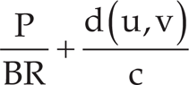
where P is the packet length, d(u, v) is the distance between u and v and c is the speed of sound in water.

The bit-rate BR was determined through the fixing of the BER (Bit Error Rate) to the value 10⁻⁵ which corresponds to a reasonable E_b/N₀ of about 47dB for 16-FSK. Fixing a BER could bring to an increasing transmission power when the distances between the nodes become larger, maintaining the same bit-rate. Instead, if we fix the transmission power the bit-rate is also affected by the necessity for an increasing time guard w.r.t. the distance between nodes (in order to avoid a more severe multi path effect). By simulations we have found a good tradeoff in terms of transmission power and time guard that allows the performance illustrated in table 1, which will be our reference scenario for the simulation of the whole system.

Table 1.

Parameters used for the three reference scenarios

	Scenario 1	Scenario 2	Scenario 3
Average node distance	7,5 m	10 m	20 m
Transceiver frequency	400 kHz	400 kHz	400kHz
Power max	35 mW	50 mW	250 mW
Modulation index M	16	16	16
Symbol time	1 ms	1 ms	1 ms
Time guard	10 μs	200 μs	0,4 ms
Bit-rate BR	3,9 kb/s	3,3 kb/s	2,8 kb/s

Another important issue is the length of the alarm packet A: the alarm packet, in fact, must contain the entire multicast tree computed by s in order to implement the smart forwarding scheme already described. In particular, this means that the length of the packet A with a standard header of 10 bytes could be fixed to 20 + 4n bytes, where n is the number of nodes in the subnetwork considered by s for the calculation of the multicast tree. Finally, the transmission time of the RTS and CTS signals τ has been set to 75μs, while the maximum packet length P₁ has been set to 40 bytes.

6. Simulations

In order to assess the efficacy of our algorithm we performed several simulations. We assume the source AUV s knows the positions of each element of the swarm, and we restrict our attention to the case where the target is a subset of the entire swarm and the source node is outside that target.

The target set consists of all the AUVs that belong to an ellipsoidal volume defined by s in the world reference frame. We now present and discuss the results collected during the execution of the following three categories of settings.

6.1 Ellipsoidal Configurations

In the first configuration a formation composed by 100 AUVs is arranged on a spherical flattened volume. The source node is located on the opposite side of the swarm with respect to the target set, which includes four nodes. On this geometrical distribution of AUVs we tried to set three different communication ranges: 7.5m, 10m, and 20m, respectively. In Figure 1 we show the result of the algorithm for the 7.5m setting.

Figure 1.

Algorithm run on the spherical flattened volume with .5m communication range

In green we can see the source node and the target set nodes, while the nodes highlighted in blue represent those involved in the signalling procedure. The arcs in red belong to the multicast tree, and the light red ellipsoid represents the target set.

In the next table we sum up the results we obtained for the three instances with a different communication range. In particular we show: the potential of the target set nodes (36, 53, 93, 94) at the end of the algorithm, which represents the time of reception of the alarm message in seconds, the number of nodes involved in the signalling procedure, the maximum number of hops between the source and the target set, and the distance (in metres) between the source and the furthest node in the target set.

Table 2.

Results for spherical flattened volume with 100 AUVs: the potential function for each node in the target set for the chosen communication ranges indicates the time of arrival (in seconds) of the alarm message

Potential function for target set	Range 7.5m	Range 10m	Range 20m nodes
p(36)	1.078 s	1.35 s	0.717 s
p(53)	1.435 s	2.508 s	1.148 s
p(93)	1.428 s	2.133 s	1.148 s
p(94)	1.296 s	1.454 s	0.931 s
Number of signalling nodes	59	73	100
Max. number of hops between source and target set	10	7	4
Max. distance between source and target set	40.06 m	40.06 m	40.06 m

We would expect that the time of reception of the alarm at the target set decreases with an increasing communication range. This should be mostly be in relation to the fact that when we increase the communication range, the number of hops between the source and the target set strictly decreases, and this effect is beneficial even if the bit-rate slows down (depending on the protocol parameters) with an increasing communication range. A more connected communication network should increase the number of nodes involved in the signalling procedure.

The simulation results in table 2 show that this intuitive behaviour is not always respected, but the protocol outcome is strongly affected by the geometrical configuration of the swarm. In particular, the intermediate range setting does not bring the expected benefits mainly because the number of hops in the tree from the source to the target set does not decrease significantly (see table 3).

Table 3.

Results for spherical flattened volume with 100 AUVs: number of hops in the tree from the source to the target set

Target set node ID	Number of hops in the tree for 7.5m	Number of hops in the tree for 10m
36	5	5
53	10	7
93	7	6
94	6	5

These outcomes suggest that it could be interesting to open a new approach, investigating the possibility of studying different topologies of the swarm that can quicken message transmission and implementing these topologies in flocking rules that try to conserve the optimal status.

We can observe that, if our alarm is critical for the life of the members of the target set, it might be worth involving all of the network and causing it to arrive as fast as possible (it would correspond to the 20m communication range). If, instead, our alarm contains a less critical message (for example if it signals important topics for the accomplishment of the swarm mission), it may be more important to preserve the communication channel for distant nodes. In this case our protocol seems effective, in the sense that the alarm transmission does not affect communications over the remaining part of the swarm.

In the second setting we used the same spherical flattened volume but with only 50 AUVs (i.e. the geometrical density of the swarm is halved). In this simulated instance of the problem the target set has cardinality two (nodes 18 and 47) and with a 7.5m communication range the network is not connected. In table 4 we sum up the results.

Table 4.

Results for spherical flattened volume with 50 AUVs: the potential function for each node in the target set for the chosen communication ranges indicates the time of arrival (in seconds) of the alarm message

Potential function for target set nodes	Range 10m	Range 20m
p(18)	1.208 s	0.441s
p(47)	1.332 s	0.719s
Number of signalling nodes	47	50
Maximum number of hops between source and target set	7	3
Maximum distance between source and target set	32.76 m	32.76 m

In the third setting a formation composed of 50 AUVs is located on an ellipsoidal volume. The source node is located in approximately the middle of the swarm. The paths computed by the algorithm running on the source node with a 10m communication range are shown in Fig. 2, with the same colour codes of Figure 1.

Figure 2.

Algorithm run on an ellipsoidal volume with 10m communication range

The target set includes seven nodes (21, 24, 32, 42, 44, 48, 49) and again with a 7.5m communication range we do not obtain a connected network. In table 5 we sum up the results.

In both settings with 50 AUVs we can see how we have fewer benefits with our procedure when the network is sparser and we have a smaller number of nodes. In fact, in both cases even with the smaller communication range a large fraction of the nodes is involved in the signalling procedure. Setting 2 is critical from this point of view, because the target set is very small and thus the ratio (#target set nodes)/(#signalling nodes) is less favourable (2/47 in setting 2 vs. 7/44 in setting 3).

Table 5.

Results for ellipsoidal volume with 50 AUVs: the potential function for each node in the target set for the chosen communication ranges indicates the time of arrival (in seconds) of the alarm message

Potential function for target set nodes	Range 10m	Range 20m
p(21)	0.516 s	0.154s
p(21)	0.516 s	0.152s
p(32)	0.503 s	0.513s
p(42)	0.523 s	0.153s
p(44)	0.5s	0.51s
p(48)	0.502s	0.512s
p(49)	0.415s	0.286s
Number of signalling nodes	44	50
Maximum number of hops between source and target set	5	3
Maximum distance between source and target set	26.13 m	26.13 m

Considering that in a real case of swarm navigation the density of nodes can change in relation to the environmental modifications, or to requests coming from the mission control, we considered evaluating how the efficiency of the algorithm is affected by such kinds of modifications.

The initial swarm configuration shown in Fig. 1 was scaled with a scaling factor varying between 0.5 and 3 (with a 0.1 step). In each simulation we considered the same three communication ranges as before: 7.5m, 10m and 20m.

Fig. 3 shows the potential of one node in the target set as a function of the scale factor. The relationship has a linear trend with random deviations. The slope of the linear trend depends on the communication range (higher for a smaller range), but it is always positive, as we would expect. Clearly for the two smaller communication ranges we could not analyse the entire scale factor interval due to a lack of connectivity across the swarm for large scaling factors.

Figure 3.

Potential of node 53 (in the target set) versus scale factor

Considering the relevance of the hop number in the potential of the target set, we presented the relationship between the scaling factor and the number of hops needed to reach the furthest node (in terms of hops) in the target set in Fig. 4.

Figure 4.

Maximum number of hops between the source and the target set versus scale factor

In Fig. 5 the amount of nodes involved in the algorithm as function of the scale factor is shown. In this case we can see that for small scaling factors (i.e. high physical density of the swarm), all of the nodes are involved in the alarm diffusion protocol. Clearly the higher the communication range, the higher the scaling factor required in order to involve less than 100 AUVs in the protocol.

Figure 5.

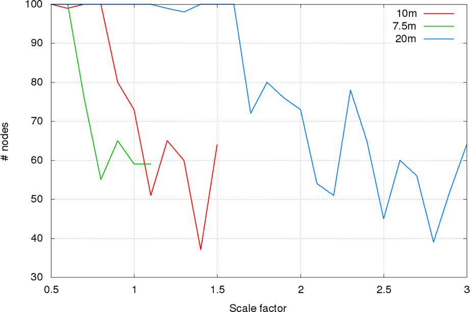
Number of nodes involved in communication versus scale factor

6.2 Ring Configuration

In practical scenarios we met situations in which the swarm reacted to external moving obstacles with an interruption of its continuity; the most common reaction is the creation of a hole inside the formation to avoid collisions. Therefore, an analysis of how the swarm density influences communication was carried out.

Unlike the previous scenario, the volume occupied by the swarm was kept constant, and we changed the density varying the amount of AUVs in it. AUVs are displaced on a planar annulus with a 10m inner radius and 50m outer radius (see Fig. 6).

Figure 6.

Algorithm run in a ring planar configuration with 294 AUVs and 7.5m communication range. The two nodes of the target set and the source are highlighted in green; red arcs belong to the alarm communication tree.

We randomly generated the instances varying the minimum allowed distance between two AUVs from 4.275m to 15m. In terms of the number of AUVs inside the ring this means a range from 30 to 294 AUVs.

Fig. 7 shows the relation between the minimum allowed distance between AUVs and the potential of a node in the target set. Again, when the minimum distance allowed is too large, we lose connectivity for small communication ranges.

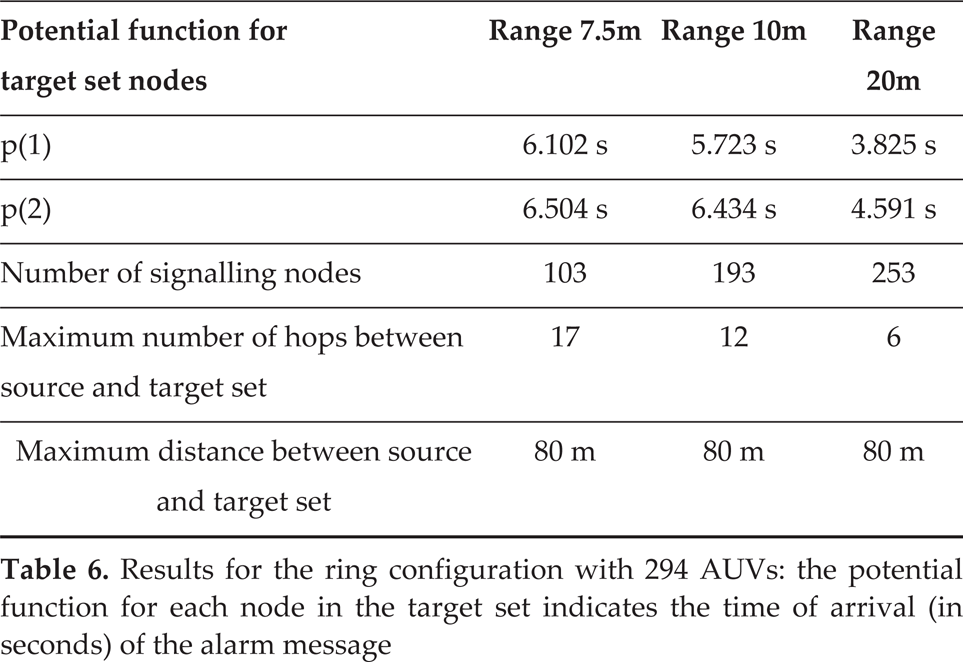
In table 6 we sum up the usual results for the combination of the densest instance, with 294 AUVs, and the smallest communication range, 7.5m. In this case we did not find any geometric anomaly at a 10m communication range.

Figure 7.

Potential of node 1 (in the target set) versus minimum allowed distance between two nodes of the swarm

Table 6.

Results for the ring configuration with 294 AUVs: the potential function for each node in the target set indicates the time of arrival (in seconds) of the alarm message

Potential function for target set nodes	Range 7.5m	Range 10m	Range 20m
p(1)	6.102 s	5.723 s	3.825 s
p(2)	6.504 s	6.434 s	4.591 s
Number of signalling nodes	103	193	253
Maximum number of hops between source and target set	17	12	6
Maximum number of hops between source and target set	80m	80m	80m

6.3 Concave Configuration

Among the many possible configurations we have considered we found of particular interest the case in which a large obstacle (i.e. a ship or a boat) creates anomalous situations where a recovery is immediately needed.

In such a case the spatial configuration determined by flocking rules results in a concave shape and the need for high priority messages (alarms) is perhaps of the outmost importance. Therefore we devoted some effort to understand which kind of anomalies could arise in these situations and possibly to define strategies to increase the robustness of the system.

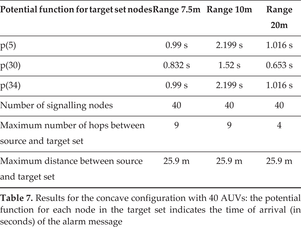
40 AUVs are displaced in a concave planar configuration that mimics the avoidance of a 15m diameter circular obstacle (see Fig. 8). Again we have run the algorithm on this configuration with the usual three communication ranges (all the instances were connected). We show the results in table 7. Again, as in our first instance as shown in Fig. 1, we have a substantial increment of the potential of the nodes in the target set for the 10m range, and again we suppose that this increment is mostly due to the fact that going from a 7.5m range to a 10m range does not change the number of hops needed to go from the source to the target set, as table 8 shows. We can also observe that the potential of nodes 5 and 34 is slightly bigger with the 20m range than with the 7.5m range; this is clearly due to the two long arcs connecting node 30 to 5 and 34.

Figure 8.

Algorithm run in a concave configuration with 40 AUVs and 7.5m communication range. The three nodes of the target set and the source node are highlighted in green; red arcs belong to the alarm communication tree.

Table 7.

Results for the concave configuration with 40 AUVs: the potential function for each node in the target set indicates the time of arrival (in seconds) of the alarm message

Potential function for target set nodes	Range 7.5m	Range 10m	Range 20m
p(5)	0.99 s	2.199 s	1.016 s
p(30)	0.832s	1.52s	0.653s
p(34)	0.99s	2.199s	1.016s
Number of signalling nodes	40	40	40
Maximum number of hops between source and target set	9	9	4
Maximum distance between source and target set	25.9m	25.9m	25.9m

Table 8.

Results for the concave configuration with 40 AUVs: number of hops in the tree from the source to the target set

Target set node ID	Number of hops in the tree for 7.5m	Number of hops in the tree for 10m
5	10	10
30	9	9
34	10	10

7. Conclusions and Next Steps

This work forms part of efforts by a single team composed by three RTOs (Research Technology Organization): namely ENEA, University of Tor Vergata, University of Perugia, besides the Italian Institute of Technology as the major funder. By means of the exploitation of the dynamic simulator, we achieved confidence that alarm management can be realized in efficient ways.

The research demonstrates the efficiency of self-adapting protocols that halt normal networking operations in alarm situations, and that are able to transmit priority information in a multihop network configuration, with overall transmission times that are compatible with the external event timing.

It is to point out the importance of the configuration control: in the intermediate communication range (10m) it can happen that for strongly irregular nodes distributions the potential of target set nodes can be affected by two different effects: the selection of long time guards and the down-grade of network connectivity. Following our analysis, both of them can be attributed to the lack of a suitable flocking rule that can ensure a topological isotropy beyond the more classical rules relevant to the distance and velocity homogeneity. This brings to local modification of the pattern regularity with severe effects on the network bandpass. In the research follow-up this point will be taken into account, introducing rules that not only refer to geometrical relationships with the closest neighbours, but also to the local density around the nodes. A potential-like function able to generate an attractor towards low-density regions could be a suitable correction.

The most convenient path for the alarm propagation was found in all of the simulations carried out. Apart from the inconvenient singularity case shown in table 2 for a 10m communication range already discussed, the alarm always reached the leaf nodes in times close not over two seconds and after not more than ten hops.

This delay is to be compared with the external event timing supposed in most of the cases to be in the order of around one minute, and that was derived by a real case. In fact, this work has given a preliminary answer to a practical problem that has been considered in the preparation of a large security project for the protection of critical infrastructures against possible asymmetric threats. The project (details are reserved) is still in its definition phase, but in this case the alarm signals could be originated not only by swarm nodes but also by external/surface sensors, able to transmit information to the most convenient node of the swarm that will operate as a gateway to other nodes of the network.

Because the test in the real underwater environment with such a number of nodes (100 or more) is beyond the possibilities of the research team, both in short and in medium terms, we intend to improve the algorithm and to test it under the conditions of the before-mentioned project using two types of approaches. First we want to increase the likeliness of the simulation with the enrichment of the navigation medium models with more environmental details (taken by the real marine environment of the project) and at the same time improve the fusion among the communication and physical simulators. Second we want to use the four vessels currently available to check the features of the physical channel and the performances of the modem realized by the team itself for swarm networks communication in real operating conditions.

The simulation refinement that will come from these tests is expected to enhance the operation of the network, especially for a fast reaction of the swarm to external conditions. A further step is represented by the introduction of the dynamic change of the configuration. The approximation of a frozen configuration to calculate the best tree is a risky approach, especially when some of the nodes on the path are close to the limit reaching range. Despite the relative slowness of the vessel navigation, some of them could become unavailable at the time the message would reach them so that the alarm-sending procedure could fail. To recover this situation we have planned a further step where the tree calculation will be made again at intermediate nodes. This could slow down the message transmission, depending on the computational power available on each node, so that some tradeoff will be needed to optimize this phase.

In addition the project is now studying and developing an integrated optical-acoustical communication network, also trying to overcome the optical limits that have been described. Depending on the performances and characteristics of the optical communication transceivers under realization, the acoustical alarm transmission time could be strongly improved up to the limit to obtain a complete optical alarm transmission in the most favourable cases (all hops within the range of an optical transmission) or to implement a partial acoustical optical transmission where the details of the protocol are still to be studied. First steps already under investigation are based on the use of an OOK modulation for optical transmission combined with a sophisticated acoustical protocol that uses the first to solve channel contents.

More advanced steps will be addressed, from the study of protocols suitable for knowledge propagation, as mentioned in [11], to the management of multizone simultaneous traffic in large networks and to the extension of the currently described protocol, and to different cases when the silence zone must be kept for a long times. This could be the case for intense, high-speed communication from a large source (like a camera) to a final target (like a gateway to a control console outside of the sea).