Indoor Slope and Edge Detection by Using Two-Dimensional EKF-SLAM with Orthogonal Assumption

Abstract

In an indoor environment, slope and edge detection is an important problem in simultaneous localization and mapping (SLAM), which is a basic requirement for mobile robot autonomous navigation. Slope detection allows the robot to find areas that are more traversable while the edge detection can prevent robot from falling. Three-dimensional (3D) solutions usually require a large memory and high computational costs. This study proposes an efficient two-dimensional (2D) solution to combine slope and edge detection with a line-segment-based extended Kalman filter SLAM (EKF-SLAM) in a structured indoor area. The robot is designed to use two fixed 2D laser range finders (LRFs) to perform horizontal and vertical scans. With local area orthogonal assumption, the slope and edge are modelled into line segments swiftly from each vertical scan, and then are merged into the EKF-SLAM framework. The EKF-SLAM framework features an optional prediction model that can automatically decide whether the application of iterative closest point (ICP) is necessary to compensate for the dead reckoning error. The experimental results demonstrate that the proposed algorithm is capable of building an accurate 2D map swiftly, which contains crucial information of the edge and slope.

1. Introduction

To perform autonomous navigation, a robot that enters an unknown environment needs to incrementally reconstruct a consistent map of the environment and simultaneously estimate its position with respect to the map so that it can continue navigating without collision or falling. In most cases, the dead reckoning method is executed to estimate the displacement of the robot, which is equipped with proprioceptive sensors, such as wheel encoders and inertial sensors. However, dead reckoning suffers from unbounded error accumulation. Therefore, external sensors (typically LRF, ultrasonic sensors, cameras, and 3D sensors) are essential not only for mapping the environment but also for the localization correction. It is noted that the data gathered from external sensors while exploring the environment are also noisy. To achieve localization and mapping simultaneously and accurately, the data from the sensors must be precisely fused to get the optimal estimation. This problem is well-known as the SLAM problem, which has attracted a lot of interest from researchers in the past decade. In [1], a brief history of the SLAM research and two influential solutions to the SLAM problem, i.e., EKF-SLAM and Rao-Blackwellized particle filters (FastSLAM), are presented. The major issues in the SLAM research, such as computational complexity, data association, and environment representation, are discussed in [2]. A general overview and detailed analysis of SLAM can also be found in [3] and [4].

Occupancy grid maps and feature-based maps are two widely adopted methods to represent the environment. Occupancy grid maps can represent arbitrary forms of the environment by dividing it into grids, where each cell of the grid is either occupied or free. However, it requires a huge amount of memory for the divided grids, and it is computationally expensive during the update process. Feature-based maps are popular in various SLAM studies due to their compactness. Points, line segments, and planes are typical features that are employed in the feature maps. Line-segment-based maps, which can represent structured environments adequately, are often employed in indoor environment applications [5, 6] due to their small memory requirement and low computational cost.

With regard to the sensors, 2D LRFs are popular in the SLAM research due to their high speed and accuracy. Another merit of using LRFs is that they are robust to variations of lighting and temperature conditions. A fixed LRF takes measurements in one plane and thus only a 2D map can be built. To acquire a 3D point cloud of the environment, some continuing or reciprocating rotation mechanisms to drive LRF have been developed by researchers in [7] and [8]. An alternative method is to fix two LRFs orthogonally to realize horizontal and vertical scans [9]. Compared with rotating mechanisms, the latter solution has some merits, such as saving energy, reducing noise, and avoiding extra vibration.

EKF and ICP, which refer to the probabilistic method and scan matching method, respectively, are the most popular algorithms employed in the SLAM research. EKF is the extended nonlinear version of the Kalman filter after linearizing the state and measurement equation via Taylor expansion. Usually, EKF-SLAM is based on features, such as points, line segments, and planes. Various successful applications or analysis of EKF-SLAM have been reported by researchers in [10] and [11]. ICP addresses the problem of estimating the optimal transformation that aligns two sets of points that partially overlap [12]. There are many variants of ICP, such as iterative dual correspondence [13] and metric-based ICP [14]. A fast 2D version of ICP has been proposed for motion estimation in [15] and is adopted in this study because of its straightforward usability.

In the case of SLAM application in indoor environments, the orthogonal assumption is a sound constraint especially for the structured buildings that feature many planes that are parallel or perpendicular to each other. By utilizing the features (typically line segments and constrained planes) scanned from these planes, a specific orientation that indicates the planes' alignment can be estimated. This assumption has been adopted in many studies to achieve good results with a limited use of sensors [16, 17] and lower computational cost [18].

As compared with a 3D map, a 2D map only carries planar information about the environment. Therefore, the memory, computational costs of manufacturing, updating, and consultation are dramatically reduced. It is mainly applied to represent indoor environments, especially neat interior corridors. However, in some buildings, even in the same floor, there are often stairs because of the height variation between different areas. Some of them are accompanied by slopes or elevators for the convenience of using wheel chairs. It is extremely important to detect these types of slopes and edges so that the robot can avoid falling and make a decision on whether it is possible to move along the slope. By using RGBD cameras or another 3D sensor, 3D SLAM technology [19, 20] is capable of mapping and updating these features with various increased costs. The cost not only increases in the mapping process but also rises in localization since the 3D feature has more parameters. To overcome it, an alternative option is to enrich the 2D map by introducing key information on the essential 3D features [21]. Using ultrasonic sensors, a slope detection system has been proposed in [22]. However, it only estimates the gradient of slope and the robot is still under the risk of falling. 2D maps that record all crucial information of slope and edge are reported in [23] and [24], by using a stereo camera and 3D LRF, respectively. These two works extract the features from 3D data and then transfer to the 2D map. The limitation is that they only generate the local map instead of integrating it into the SLAM algorithm to create the global map necessary for global path planning during autonomous navigation.

In this paper, we present an ICP-assisted line segment-based EKF-SLAM framework to construct 2D maps that record essential information on slopes and edges. The proposed algorithm uses an odometer and two fixed LRFs as the main sensors. The horizontally placed LRF is used for the traditional planar scanning that is parallel to the ground, whereas the vertically fixed LRF is used to monitor the ground in front of the robot to detect slopes and edges. There are three main contributions that result from this study. First, a 2D ICP algorithm is applied to evaluate the dead reckoning result and make the decision whether to step further to compensate for error. Second, the slopes and edges detected in the vertical scans are modelled into 2D line segments with the angular parameter estimated by local orthogonal assumption. Third, a method to integrate and update the extracted features (the line segments that represent the slope and edge) into the EKF-SLAM framework is proposed.

The rest of this paper is structured as follows. Section 2 describes the mobile robot and system architecture developed in this research. The algorithm of ICP-assisted line-segment-based EKF-SLAM is introduced in section 3; it consists of the line segments extraction, 2D EKF-SLAM,

and ICP application. Section 4 presents the method for extracting the features of the slope and edge and integrating them into the EKF-SLAM framework. The experiment that verifies the efficiency of the proposed algorithm is detailed in the section 5. Section 6 includes several conclusions and proposed future work.

2. Robot platform and system architecture

This section first introduces the mobile robot and its equipped sensors. Then, the system architecture is briefly explained.

2.1 Robot platform and sensors

Figure 1 shows the experimental mobile robot employed in this research. This robot is developed by assembling two LRFs (both manufactured by Hokuyo Co. Ltd) on the platform (Plat_F1, Japan Systems Design Co. Ltd). LRF1 (UHG-08LX) is attached on the front part of the bottom base to fulfil the horizontal scans. The second layer is placed above the base to support the PC. An aluminium frame is fixed on the forefront of the second layer to vertically sustain LRF2 (UBG-04LX-F01) at an appropriate height so that the ground can be detected well enough by the vertical scanning. The odometer, which consists of two encoders (RE20F_100_200, Copal Electronics), is installed next to the rear wheels to estimate the displacement of the robot.

Figure 1.

The mobile robot and sensors used for the experiments

2.2 System architecture

The whole system architecture can roughly be divided into three procedures with regard to the data read from three sensors, as shown in Figure 2.

Figure 2.

Overview of the system architecture

The dead reckoning process is executed to estimate the transformation of the robot during the time interval between step (t − 1) and step t. After transformation by utilizing the estimation result, a copy of the horizontal scan S_h (t) is applied to match the former horizontal scan S_h (t − 1) in order to evaluate the quality of the dead reckoning result. Based on this evaluation, the decision is made on whether ICP must be executed to compensate for the odometer error. Finally, the EKF prediction process is conducted by utilizing the original or compensated dead reckoning result.

Meanwhile, the line segments are extracted from the horizontal scan and then imported into the EKF-SLAM to execute the feature association and correction. In addition, the orthogonal angle is estimated based on the extracted line segments if any slope or edge has been detected in the vertical scan process.

Other than the horizontal procedure, the orthogonal estimation is conducted at every step of the vertical scan S_v(t) to ensure that the central axis of the scan plane is parallel to the ground. The vertical feature extraction is mainly utilized in the line segments scanned from the slope and the points that are next to the edge. With the angular parameter provided by horizontal orthogonal estimation, the vital information of vertical features can be estimated and then transported into the EKF-SLAM for feature association and correction.

3. ICP assisted line segments based EKF-SLAM

The first two parts of this section are brief reviews of our previous work on a 2D line segment-based EKF-SLAM algorithm [6]. The last subsection briefly introduces the ICP algorithm. Then, an ICP-based EKF-SLAM prediction model is detailed. Finally, a simple selection to pick a suitable prediction model is proposed.

3.1 Line segments extraction

A good line extraction algorithm is expected to extract the parameters of the straight line segments from noisy raw points scanned by LRF accurately and swiftly. There are many famous algorithms that have been proposed in the past including incremental, split and merge, Hough transform, line regression, RANSAC, and expectation maximization algorithm. Based on the comparison between these algorithms conducted in [25], the split and merge is employed in this study because of its superior speed and accuracy. As the name indicates, it first splits raw points into collinear clusters and then fits and merges the line segments.

3.2 Line segments based EKF-SLAM

EKF-SLAM algorithm utilizes a large state vector to record the localization (robot pose state P) and mapping result (feature state F). The state vector is modelled by a Gaussian variable and maintained by the EKF through prediction, feature association, correction, and new feature addition.

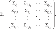
At time t, the state vector considering line segments as the features is expressed as follows:

${\mu }_t={\left(\begin{array}{cccc}{P}_t& F_1& \cdots & F_n\end{array}\right)}^{\mathrm{T}},$

(1)

where the subscript “n” stands for “feature number.” As shown in Figure 3, the robot pose and the parameters of the features with respect to the global frame O-X_GY_G are as follows:

Figure 3.

Geometrical relationship between the robot pose and feature parameters

$P_t=\left(\begin{array}{ccc}{x}_{p(t)}& y_{p(t)}& {\theta }_{p(t)}\end{array}\right),\hspace{0.17em}\hspace{0.17em}\hspace{0.17em}{F}_i=\left(\begin{array}{cc}{\rho }_{f(i)}& {\alpha }_{f(i)}\end{array}\right).$

(2)

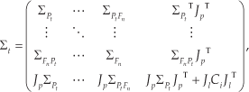
where the subscript “p” stands for “pose,” and “f” stands for “feature.” Moreover, the covariance matrix of state vector is expressed as follows:

${\Sigma }_t=\left(\begin{array}{cccc}{\Sigma }_{P_t}& {\Sigma }_{P_t{F}_1}& \cdots & {\Sigma }_{P_t{F}_n}\\ {\Sigma }_{F_1{P}_t}& {\Sigma }_{F_1}& \cdots & {\Sigma }_{F_1{F}_n}\\ ⋮& ⋮& \ddots & ⋮\\ {\Sigma }_{F_n{P}_t}& {\Sigma }_{F_n{F}_1}& \cdots & {\Sigma }_{F_n}\end{array}\right).$

(3)

The endpoints of line segments are stored and updated out of the EKF frame.

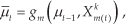
3.2.1 Dead reckoning based EKF-SLAM prediction

EKF-SLAM prediction is a procedure to estimate the transformation of robot pose between two steps such as from time (t-1) to time t. Based on the kinematic model shown in Figure 4, the predicted new pose of the robot as derived from the odometer-based dead reckoning is calculated as follows:

Figure 4.

Kinematic model of robot

${\bar{\mu }}_t=g_{dr}\left({\mu }_{t-1},u_t\right)\text{\hspace{0.17em},}$

(4)

${\bar{x}}_{p\left(t\right)}=x_{p\left(t-1\right)}-\frac{\left(\Delta R+\Delta L\right)}{2}\text{sin}({\theta }_{p(t-1)}+\frac{\left(\Delta R-\Delta L\right)}{2D}),$

(5)

${\bar{y}}_{p(t)}=y_{p(t-1)}+\frac{\left(\Delta R+\Delta L\right)}{2}\text{cos}({\theta }_{p(t-1)}+\frac{\left(\Delta R-\Delta L\right)}{2D}),$

(6)

${\bar{\theta }}_{p(t)}={\theta }_{p(t-1)}+\frac{\left(\Delta R-\Delta L\right)}{D}\hspace{0.17em}\hspace{0.17em},$

(7)

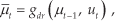
where D stands for the distance between the rear wheels, u_t = (ΔR ΔL) denotes the travel distance of wheels measured by the odometer during the time interval, ΔR corresponds to the right wheel, while ΔL stands for the left one. The corresponding covariance matrix of the odometer measurement is as follows:

$C_w=\left(\begin{array}{cc}{\sigma }_{\Delta R}^2& 0\\ 0& {\sigma }_{\Delta L}^2\end{array}\right).$

(8)

The covariance matrix of state vector is updated by the equation given below:

${\bar{\mathrm{\Sigma }}}_t=G_p{\mathrm{\Sigma }}_{t-1}{G}_p^{\mathrm{T}}+G_w{C}_w{G}_w^{\mathrm{T}},$

(9)

with the Jacobi matrices G_p=∂g_dr(μ_t−1, u_t)/∂μ_t−1 and G_w=∂ g_dr(μ _t -1, u_t) / ∂ u_t

This typical dead reckoning-based prediction model usually performs very well when the robot is moving at low rotational speeds with no serious slippage occurring. Another merit is that it requires a low computational cost because of its simplicity.

3.2.2 EKF-SLAM features association

After the horizontal scan, the LRF explores the environment at time t, with respect to horizontal robot frame O-X_RY_R (marked as frame R_h), a number of line segments are extracted as the measurements:

$z_i={\left(\begin{array}{cc}{\rho }_{l(i)}^{R_h}& {\alpha }_{l(i)}^{R_h}\end{array}\right)}^{\mathrm{T}},i=0,1\dots m,$

(10)

with the corresponding covariances:

$C_i=\left(\begin{array}{cc}{\sigma }_{{\rho }_{l(i)}^{R_h}}^2& {\sigma }_{{\rho }_{l(i)}^{R_h}{\alpha }_{l(i)}^{R_h}}\\ {\sigma }_{{\alpha }_{l(i)}^{R_h}{\rho }_{l(i)}^{R_h}}& {\sigma }_{{\alpha }_{l(i)}^{R_h}}^2\end{array}\right),i=0,1\dots m.$

(11)

Some of these measurements are scanned from the same objects that have been stored as features in the state vector. The main task of feature association is to find and associate these types of re-observed features so that the EKF-SLAM can correct the predicted state by comparing the measurements and stored features.

For jth stored feature, the estimated observation based on the predicted state can be calculated as follows:

$\begin{array}{c}\hspace{0.17em}\hspace{0.17em}{\widehat{z}}_j=\left(\begin{array}{c}{\widehat{\rho }}_{f\left(j\right)}^{R_h}\\ {\widehat{\alpha }}_{f\left(j\right)}^{R_h}\end{array}\right)=h\left({\bar{\mu }}_t\right)\\ =\left(\begin{array}{c}{\rho }_{f(j)}-{\bar{x}}_{p(t)}\text{cos}{\alpha }_{f(j)}-{\bar{y}}_{p(t)}\text{sin}{\alpha }_{f(j)}\\ {\alpha }_{f(j)}-{\bar{\theta }}_{p(t)}\end{array}\right).\end{array}$

(12)

The corresponding covariance matrix of ${\widehat{z}}_j$ is as follows:

${\widehat{C}}_j=H_j{\bar{\Sigma }}_t{H}_j{}^{\mathrm{T}}$

(13)

with the Jacobi matrix $H_j=\partial h({\bar{\mu }}_t)/\partial {\bar{\mu }}_t$ and ${\bar{\Sigma }}_t$ is the latest covariance matrix of the state vector.

To associate measurements with estimated observations, from all possible line pairs, the pairs that have similar parameters are firstly picked out by simply comparing the differences of their parameters with the preset thresholds. Then, for each picked pair that contains two lines, the shorter line is marked as l₁ while the longer line is marked as l₂. The length of l₂ is given by L₂. Along the direction of l₂, the distances from the endpoints of l1 to the center of l₂, which are given by d_ce1 and d_ce2 respectively, are calculated. If either of d_ce1 and d_ce2 is smaller than L₂ l₂, the overlap between l₁ and l₂ is confirmed and the pair will be treated as a candidate association pair, as shown in Figure 5.

Figure 5.

Overlap confirmation of two line segments

After a series of candidate association pairs $\left\{\left(z_i,{\widehat{z}}_j\right),\hspace{0.17em}\dots \right\}$ can be picked out. And the Mahalanobis Distance of each pair is calculated as given below:

$d_{ij}={\left(z_i-{\widehat{z}}_j\right)}^{\mathrm{T}}{\left(C_i+{\widehat{C}}_j\right)}^{-1}\left(z_i-{\widehat{z}}_j\right)\hspace{0.17em}.$

(14)

Between the calculated results of the pairs, the minimum value d_min is compared with an artificial criterion χ².

$d_{min}<{\chi }^2.$

(15)

If this judgment (15) is satisfied, the corresponding pair is successfully associated. After the correction procedure based on this associated pair is executed, another iteration of feature association will be carried out until no more pair can be associated.

3.2.3 EKF-SLAM correction

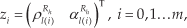
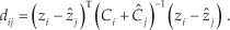
For the observation z_i that has been associated with the feature F_j, EKF-SLAM will implement the correction process to the state vector and its covariance matrix. The EKF correction process is typically written as follows:

$K_j={\bar{\mathrm{\Sigma }}}_t{H}_j{}^{\mathrm{T}}{\left(C_i+{\widehat{C}}_j\right)}^{-1}\hspace{0.17em},$

(16)

${\mu }_t={\bar{\mu }}_t+K_j\left(z_i-{\widehat{z}}_j\right),$

(17)

${\mathrm{\Sigma }}_t=\left(I-K_j{H}_j\right){\bar{\mathrm{\Sigma }}}_t\hspace{0.17em}.$

(18)

K_j is usually called Kalman gain, which is calculated by utilizing the uncertainties of the real measurements and the estimated observations. After the Kalman gain has been calculated, the state vector and corresponding covariance are updated by (17) and (18).

3.2.4 EKF-SLAM new feature addition

For the measurement z_i that has failed to associate with any stored features, EKF-SLAM will treat it as a new detected feature. Thus z_i will become the (n+1)th feature F_n+1 in the state vector:

$\begin{array}{c}\hspace{0.17em}\hspace{0.17em}{F}_{n+1}=\left(\begin{array}{c}{\rho }_{f(n+1)}\\ {\alpha }_{f(n+1)}\end{array}\right)=f\left(P_t,z_i\right)\\ \hspace{0.17em}=\left(\begin{array}{c}{\rho }_{l(i)}^{R_h}+x_{p(t)}\text{cos}{\alpha }_{f(n+1)}+y_{p(t)}\text{sin}{\alpha }_{f(n+1)}\\ {\theta }_{p(t)}+{\alpha }_{l(i)}^{R_h}\end{array}\right).\end{array}$

(19)

Moreover, the covariance matrix of the state vector also has to be augmented as follows:

${\mathrm{\Sigma }}_t=\left(\begin{array}{cccc}{\mathrm{\Sigma }}_{P_t}& \cdots & {\mathrm{\Sigma }}_{P_t{F}_n}& {\mathrm{\Sigma }}_{P_t}{}^{\mathrm{T}}{J}_p{}^{\mathrm{T}}\\ ⋮& \ddots & ⋮& ⋮\\ {\mathrm{\Sigma }}_{F_n{P}_t}& \cdots & {\mathrm{\Sigma }}_{F_n}& {\mathrm{\Sigma }}_{F_n{P}_t}{J}_p{}^{\mathrm{T}}\\ J_p{\mathrm{\Sigma }}_{P_t}& \cdots & J_p{\mathrm{\Sigma }}_{P_t{F}_n}& J_p{\mathrm{\Sigma }}_{P_t}{J}_p{}^{\mathrm{T}}+J_l{C}_i{J}_l{}^{\mathrm{T}}\end{array}\right),$

(20)

where J =∂f(P_t, z_i)/∂P_t and J_l =∂f(P_t, z_i)/∂z_i are the Jacobi matrices that linearize the new feature with respect to robot pose and measurement variables, respectively.

3.3 Dead reckoning result evaluation and ICP compensation

The prediction procedure is critical for EKF-SLAM since it usually has a great influence on the subsequent feature association. In spite of its high speed, pure dead reckoning-based prediction is risky because of the unpredictable slippage and increasing linearization error of the kinematic model when the robot increases its rotational speed. Some fatal errors may lead to the divergence of EKF-SLAM. To overcome this inconvenience and make the prediction more robust, ICP is introduced to evaluate the dead reckoning result and to compensate it when necessary.

3.3.1 ICP

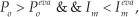
In general, ICP is an iterative algorithm that iteratively finds correspondences between two given scans, and it calculates a transformation that minimizes the distance between corresponding points until the termination condition is satisfied [26]. A fast 2D version ICP method, discussed in [15], is adopted in this study. For each iteration, it calculates the Euclidean squared distance for every possible combination of points in two scans and establishes the correspondence index based on the traditional closest point rule. The outliers are detected and discarded from valid correspondence if their closest distance is over a given rejection threshold E_rej. Finally, the transformation parameters are calculated by minimizing a general matching index I_m, which is formulated by the following equation:

$I_m=\frac{{{\displaystyle \sum }}_{i=0}^{n_c}{e}_i}{n_c{P}_o},$

(21)

where e_i is the Euclidean squared distance between the ith corresponding points, n_c stands for the number of valid correspondences, and P_o is the overlapping degree.

3.3.2 ICP based EKF-SLAM prediction

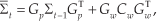
To estimate the accurate transformation of the robot pose X_m(t)= (Δ_xm(t) Δy_m(t) Δθ_m(t))^T between time (t-1) and time t, ICP is applied to match horizontal scans S_h(t-1) and S_h(t). It is noted that instead of referring to the global frame, X_m(t) is a relative transformation with respect to the robot frame at time (t-1). The initial estimation X⁰_m(t) is given by the odometer-based dead reckoning result as follows:

$\mathrm{\Delta }{\theta }_{m(t)}^0=\frac{\left(\mathrm{\Delta }R-\mathrm{\Delta }L\right)}{D},$

(22)

$\mathrm{\Delta }{x}_{m(t)}^0=-\frac{\left(\mathrm{\Delta }R+\mathrm{\Delta }L\right)}{2}\sin \left(\mathrm{\Delta }{\theta }_{m(t)}^0\right),$

(23)

$\mathrm{\Delta }{y}_{m(t)}^0=\frac{\left(\mathrm{\Delta }R+\mathrm{\Delta }L\right)}{2}\text{cos}\left(\mathrm{\Delta }{\theta }_{m(t)}^0\right).$

(24)

The rejection threshold E_rej is a vital parameter for ICP implementations. A low value may lead to a bad convergence, whereas a large value tends to deteriorate the result. For each point in S_h (t-1) the maximum rejection threshold E_rej^max is initialized as follows:

$E_{rej}^{max}=\left({\chi }_{0.99}^2\right)+E_r={\left(6.63\sigma \right)}^2+E_s,$

(25)

where σ corresponds to standard deviation of the scanned point and E_s stands for possible slippage error, which is determined by taking robot speed and time interval into consideration. The rejection threshold is updated by the algorithm named relative motion threshold (RMT), proposed in [27], when it is bigger than a fixed minimum criterion:

$E_{rej}^{min}=\left({\chi }_{0.99}^2\right)={\left(6.63\sigma \right)}^2.$

(26)

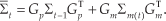
After ICP has run k iterations and arrived at a fit solution $X_{m(t)}^k$ , the corresponding covariance Σ_m(t) has to be determined with the intention of EKF-SLAM prediction. By utilizing a closed-form estimation method [28], the covariance is derived as follows:

${\mathrm{\Sigma }}_{m(t)}={\left(\frac{{\partial }^2{I}_m}{\partial X^2}\right)}^{-1}\frac{{\partial }^2{I}_m}{\partial S\partial X}\mathrm{\Sigma }\left(S\right){\frac{{\partial }^2{I}_m}{\partial S\partial X}}^{\mathrm{T}}{\left(\frac{{\partial }^2{I}_m}{\partial X^2}\right)}^{-1},$

(27)

where Σ(S) stands for the covariance of measurements S_h(t-1) and S_h(t). The necessary derivatives ${\partial }^2{I}_m/\partial X^2$ and ${\partial }^2{I}_m/\partial S\partial X$ can be easily computed in a closed form based on the analytical solution of X_m(t) as stated in [15].

Finally, the ICP-based new predicted pose of the robot is calculated as follows:

${\bar{\mu }}_t=g_m\left({\mu }_{t-1},\hspace{0.17em}{X}_{m(t)}^k\right)\hspace{0.17em},$

(28)

${\bar{x}}_{p\left(t\right)}=x_{p\left(t-1\right)}+\mathrm{\Delta }{x}_{m(t)}^k\text{cos}{\theta }_{p(t-1)}-\mathrm{\Delta }{y}_{m(t)}^k\text{sin}{\theta }_{p(t-1)}$

(29)

${\bar{y}}_{p\left(t\right)}=y_{p\left(t-1\right)}+\mathrm{\Delta }{x}_{m(t)}^k\text{sin}{\theta }_{p(t-1)}+\mathrm{\Delta }{y}_{m(t)}^k\text{cos}{\theta }_{p(t-1)}$

(30)

${\bar{\theta }}_{p(t)}={\theta }_{p(t-1)}+\mathrm{\Delta }{\theta }_{m(t)}^k.$

(31)

The covariance matrix of the state vector is updated by the following equation:

${\bar{\mathrm{\Sigma }}}_t=G_p{\mathrm{\Sigma }}_{t-1}{G}_p^{\mathrm{T}}+G_m{\mathrm{\Sigma }}_{m(t)}{G}_m^{\mathrm{T}}.$

(32)

with the Jacobi matrices $G_p=\partial g_m({\mu }_{t-1},X_{m(t)}^k)/\partial {\mu }_{t-1}$ and $G_m=\partial g_m({\mu }_{t-1},X_{m(t)}^k)/\partial X_{m(t)}^k$ .

3.3.3 Optional EKF-SLAM prediction

Although the ICP-based EKF prediction gives a more robust result, it is associated with a much higher computational cost than dead reckoning for both the iterations and the final covariance estimation of the ICP result. Therefore, an optional EKF-SLAM prediction model is proposed by selecting two addressed models based on the evaluation of the dead reckoning result.

To verify whether the dead reckoning result is precise enough, only one iteration of ICP is executed with the rejection criterion E_rej^eva, which is determined by the E_rej^min plus one small tolerance E_T. The overlapping degree P_o and matching index I_m can be found after a single iteration. Then, a simple judgment is conducted:

$P_o>P_o^{eva}\&\&\hspace{0.17em}{I}_m<I_m^{eva},$

(33)

where P_o^eva is the overlapping threshold and I_m^eva is the error index threshold. The judgment (33) is satisfied only when two successive scans overlap mostly with low errors, which means the dead reckoning result provides a good estimation. Thus, if the judgment is satisfied, the faster dead reckoning-based EKF prediction is going to be conducted. Otherwise, a further ICP iteration has to be employed with the reinitialized rejection threshold E_rej^max so that ICP-based EKF prediction will be executed to guarantee the robustness of the prediction.

4. Slope and edge feature in EKF-SLAM

4.1 Vertical feature extraction and integration

The basic concept of feature detection and extraction in the vertical scan is shown in Figure 6. A slope marked as ABCD (corresponding to four corners) is placed next to an edge marked as GH. When LRF2 finds a line segment SL scanned from the slope, partial information of the slope can be extracted by decomposing vector $\overrightarrow{SL}$ into $\overrightarrow{SN}$ and $\overrightarrow{NL}$ . The distance between the robot and the edge can be estimated from the detected edge points E by similar decomposition. For correct decomposition, the exact orientation of the slope and edge line needs to be known in advance; this can be solved by utilizing the horizontal scanned line segments with the orthogonal assumption.

Figure 6.

Slope and edge detection by the vertical scan

Since this research focuses on the 2D map, a top view of Figure 6 is represented in Figure 7. To simplify the explanation of the slope and edge detection, the vertical scanning plane is designed to be in the same plane as OY_RZ_R. The main extraction procedure is executed in horizontal frame OX_RY_R (marked as frame Rh) and vertical frame OYRZR (marked as frame R_v).

Figure 7.

Simplified top view of the vertical feature detection

4.1.1 Orthogonal angle estimation

The exact orientation of the slope and edge line is estimated with a well-known geometrical constraint named orthogonal assumption. When a slope or edge is detected by LRF2, the local orthogonal angle α _o ^Rh and its variance ${\sigma }_{{\alpha }_o^{R_h}}^2$ are calculated [29] based on the horizontal scanned line segments as shown in Figure 8. Since the slope is typically located in the corridor, α _o ^Rh can precisely indicate the orientation of the slope with respect to the robot's horizontal frame O-X_RY_R.

Figure 8.

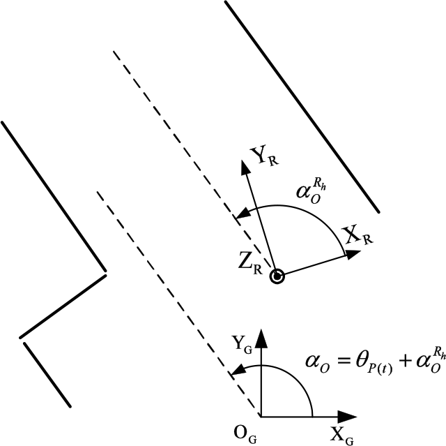
Orthogonal angle estimation of the horizontal scan

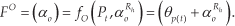
The global orthogonal angle α _o can be added to the EKF-SLAM state vector μ _t as a feature F^O.

$F^O=\left({\alpha }_o\right)=f_O\left(P_t,{\alpha }_o^{R_h}\right)=\left({\theta }_{p(t)}+{\alpha }_o^{R_h}\right).$

(34)

Moreover, the covariance matrix of the state vector can be augmented in a similar way as in Equation (20), and it will not be detailed here.

Another application of the orthogonal assumption is the vertical scan correction. The central axis of LRF2 is designed to be parallel to the ground. However, even in the indoor environment, the ground where the robot is moving cannot be absolutely flat and smooth. The space between tiles can easily affect the parallelism, which may lead to errors during the vertical feature extraction. To overcome this problem, orthogonal estimation of the vertical scan is executed in every step to compensate for the error. This is feasible because most features in the vertical scan plane, such as ceiling, wall, and ground, are parallel or perpendicular to each other as shown in Figure 9.

Figure 9.

Vertical scanning plane and features of interest

4.1.2 Vertical scan classification

Before starting to build the line segment model of the slope and edge, the vertical scanned data need to be classified under the frame of LRF2. Basically, the classification is executed after extraction of line segments. The slope line segment can be easily found by checking the parameters such as length, range, angle, and covariance. For edge point detection, two situations must be considered. The first situation is that the edge point is the intersection point of the ground line and down slope line segment, as shown in Figure 9. The second situation is shown in Figure 10; a short ground line segment has been detected without a following slope line segment. In this case, the remote endpoint of the ground line segment will be treated as the edge point if the incidence angle of its ray is bigger than a given threshold ω ^E _T and no points are scanned from other features in the range of ω ^E _T to the edge point.

Figure 10.

Second situation of edge point detection

4.1.3 Line segments modeling and integration of edge

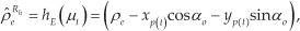
In a 2D map, the key characteristic of the edge can be perfectly represented by the edge line, which is marked as line segment HG in Figure 7. However, the vertical scan plane can only detect one edge point that is supposed to be the closest one to the real edge line. Thus, as shown in Figure 11, the edge feature F^E that is going to be added into the state vector can be estimated by utilizing the single detected edge point E, the robot pose P_t, and the corresponding orthogonal angle α _o as follows:

Figure 11.

Edge line estimation based on the edge point E

$\begin{array}{c}\hspace{0.17em}\hspace{0.17em}\hspace{0.17em}{F}^E=\left({\rho }_e\right)=f_E\left(P_t,F^O,y_e^R\right)\\ =\left(y_e^R\text{sin}\left({\alpha }_o-{\theta }_{p(t)}\right)+x_{p(t)}\text{cos}{\alpha }_o+y_{p(t)}\text{sin}{\alpha }_o\right).\end{array}$

(35)

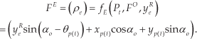
The covariance matrix of the state vector also has to be augmented as follows:

$\begin{array}{c}\hspace{0.17em}{\mathrm{\Sigma }}_t=\left(\begin{array}{ccc}{\mathrm{\Sigma }}_{(P_t{F}^O)}& {\mathrm{\Sigma }}_{(P_t{F}^O)F_i}& {\mathrm{\Sigma }}_{(P_t{F}^O)F^E}\\ {\mathrm{\Sigma }}_{F_i(P_t{F}^O)}& {\mathrm{\Sigma }}_{F_i}& {\mathrm{\Sigma }}_{F_i{F}^E}\\ {\mathrm{\Sigma }}_{F^E(P_t{F}^O)}& {\mathrm{\Sigma }}_{F^E{F}_i}& {\mathrm{\Sigma }}_{F^E}\end{array}\right)\\ =\left(\begin{array}{ccc}{\mathrm{\Sigma }}_{(P_t{F}^O)}& {\mathrm{\Sigma }}_{(P_t{F}^O)F_i}& {\mathrm{\Sigma }}_{(P_t{F}^O)}{}^{\mathrm{T}}{J}_{\mu }{}^{\mathrm{T}}\\ {\mathrm{\Sigma }}_{F_i(P_t{F}^O)}& {\mathrm{\Sigma }}_{F_i}& {\mathrm{\Sigma }}_{F_i(P_t{F}^O)}{J}_{\mu }{}^{\mathrm{T}}\\ J_{\mu }{\mathrm{\Sigma }}_{(P_t{F}^O)}& J_{\mu }{\mathrm{\Sigma }}_{(P_t{F}^O)F_i}& J_{\mu }{\mathrm{\Sigma }}_{(P_t{F}^O)}{J}_{\mu }{}^{\mathrm{T}}+J_y{C}_y{J}_y{}^{\mathrm{T}}\end{array}\right)\end{array}$

(36)

where C_y is the variance of the measurement y^R_e, the Jacobi matrices $J_{\mu }=\partial f_E\left(P_t,F^O,y_e^R\right)/\partial (P_t,F^O)$ and

${\mathrm{\Sigma }}_{(P_t{F}^O)}=\left(\begin{array}{cc}{\mathrm{\Sigma }}_{P_t}& {\mathrm{\Sigma }}_{P_t{F}^O}\\ {\mathrm{\Sigma }}_{F^O{P}_t}& {\mathrm{\Sigma }}_{F^O}\end{array}\right).$

(37)

The first added edge feature F^E is incomplete because it has no length with only one endpoint instead of two. This problem will be solved when another edge point is scanned and then the length can be estimated.

4.1.4 Line segments modeling and integration of slope

There are several key characteristics of slope such as width, gradient, length, and location. The location and width can be represented by the slope start line, which can be treated as line segment AB in Figure 7. The estimation of slope start line, however, differs from the edge line estimation. Instead of finding a point that is closest to the slope start line, the intersection point between the scanned slope line segment and ground is adopted. This is because the start line may not be scanned even when some line segment is scanned from the slope, as shown in Figure 12.

Figure 12.

Slope is detected without scanning the start line

From the geometrical relationship shown in Figure 13 (a), the distance y_s^R, which is measured from robot origin to the intersection point in Y_R axis direction, can be calculated by using the robot frame height h_R and the scanned slope line segment l_sl ^Rv in the plane O-Y_RZ_R as

Figure 13.

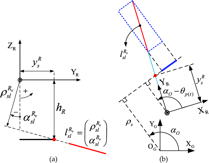
Slope start line and scanned area estimation

$y_s^R=\frac{{\rho }_{sl}^{R_v}-h_R\text{cos}{\alpha }_{sl}^{R_v}}{\text{sin}{\alpha }_{sl}^{R_v}},$

(38)

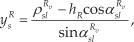
where α_sl^Rv is the angular parameter of l_sl^Rv with respect to the negative Z_R axis and is measured positive in counterclockwise direction. After y_s^R has been estimated, the slope feature F^S, which contains the distance parameter of slope start line, can be calculated as follows:

$\begin{array}{c}\hspace{0.17em}\hspace{0.17em}\hspace{0.17em}{F}^S=\left({\rho }_s\right)=f_S\left(P_t,F^O,y_s^R\right)\\ =\left(y_s^R\text{sin}\left({\alpha }_o-{\theta }_{p(t)}\right)+x_{p(t)}\text{cos}{\alpha }_o+y_{p(t)}\text{sin}{\alpha }_o\right).\end{array}$

(39)

Moreover, the covariance matrix of the state vector can be augmented in a similar way as with the edge line.

The partially discovered slope area can be determined by projecting the endpoints of l_sl^Rv along and perpendicular with the orthogonal angle. The area can be found as the blue dots plotted in Figure 13 (b). It will be augmented when another line segment is scanned from the same slope.

The last key characteristc of the slope is the gradient. From the slope model plotted in Figure 14, the geometric relationship between the slope gradient tan α _s and the scanned line angle α_sl^Rv can be found as follows:

Figure 14.

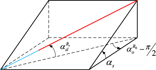
Slope model with the scanned slope line segment

$\text{tan}{\alpha }_s=\frac{\text{tan}{\alpha }_{sl}^{R_v}}{\text{cos}{\alpha }_o^{R_h}},$

(40)

where α ^Rh _o is the local orthogonal angle that has been discussed before. The slope gradient can be excluded from the EKF-SLAM frame because it is independent of the coordinate transformation in 2D frame. From every vertical scan that finds the same slope, the slope gradient tanα_s can be updated by a simple independent one-dimensional EKF with the observation Equation (40).

Until this point, three necessary characteristics of edge and slope have been successfully integrated into 2D EKF-SLAM frame. They are treated as one set but added as three individual features because slope and edge may not be detected simultaneously. Other features such as the endpoints are stored and updated out of EKF framework.

4.2 Vertical feature association and correction

Although a rough EKF processing of vertical features can be found in Figure 2, a detail flowchart is plotted in Figure 15 because the feature association of orthogonal angle and vertical feature (edge or slope) are dependent; vertical features differ from the horizontal features. For a stored orthogonal angle ao and its corresponding edge and slope, the estimated observations are as follows:

Figure 15.

The detail flowchart of the vertical features process in the EKF-SLAM frame

${\widehat{\alpha }}_o^{R_h}=h_O\left({\mu }_t\right)=\left({\alpha }_o-{\theta }_{p(t)}\right),$

(41)

${\widehat{\rho }}_e^{R_h}=h_E\left({\mu }_t\right)=\left({\rho }_e-x_{p\left(t\right)}\text{cos}{\alpha }_o-y_{p(t)}\text{sin}{\alpha }_o\right),$

(42)

${\widehat{\rho }}_s^{R_h}=h_S\left({\mu }_t\right)=\left({\rho }_s-x_{p\left(t\right)}\text{cos}{\alpha }_o-y_{p(t)}\text{sin}{\alpha }_o\right).$

(43)

Moreover, the estimation of their corresponding covariance can be expressed in a general equation as follows:

${\widehat{C}}_X=H_X{\mathrm{\Sigma }}_t{H}_X{}^{\mathrm{T}},$

(44)

where Jacobi matrix $H_X=\partial h_X({\mu }_t)/\partial {\mu }_t$ and the subscript X can stand for each feature. The association between measurement z_X and estimated observation ${\widehat{z}}_X$ is based on their Mahalanobis distance:

$d_X={\left(z_X-{\widehat{z}}_X\right)}^{\mathrm{T}}{\left(C_X+{\widehat{C}}_X\right)}^{-1}\left(z_X-{\widehat{z}}_X\right)<{\chi }^2.$

(45)

When a vertical feature has been detected in the scan, a local horizontal orthogonal angle α_o^Rh is firstly going to be estimated as the measurement and then will try to associate the measured angle with a stored orthogonal angle. If no stored orthogonal angle can be associated with this measurement, the local orthogonal angle and detected vertical feature will be added as a new set of features. Otherwise, the stored vertical feature that corresponds to the associated α_o will try to associate with the detected vertical features. If the vertical feature association fails, the orthogonal angle and detected vertical features are still going to be added as a new set of features. If the association is successful, the EKF correction will be executed based o _t n the associated features as follows:

$K_X={\mathrm{\Sigma }}_t{H}_X{}^{\mathrm{T}}{\left(C_X+{\widehat{C}}_X\right)}^{-1},$

(46)

${\mu }_t={\mu }_t+K_X\left(z_X-{\widehat{z}}_X\right),$

(47)

${\mathrm{\Sigma }}_t=\left(I-K_X{H}_X\right){\mathrm{\Sigma }}_t\hspace{0.17em}.$

(48)

5. Experiment and result

5.1 Experimental environment

The experiment was conducted in a real environment that consists of crossroad and corridors, as shown in Figure 16. Three boxes (marked as Box 1, 2, 3) are intentionally placed along the long and straight corridor to add more detectable features to the environment. There are two slopes and one edge in the experimental environment. Slope 1 is a downslope accompanied with an edge, while Slope 2 is an upslope next to the stairs. Figure 17 gives a detailed view of these two slopes. The robot is controlled to move roughly along the green dashed line (sketch, not the exact route) and finally come back to the initial position as shown in Figure 16. There are a total of 700 steps conducted in this experiment. For each step, incremental encoder data, a horizontal scan, and a vertical scan are recorded.

Figure 16.

Experimental environment

Figure 17.

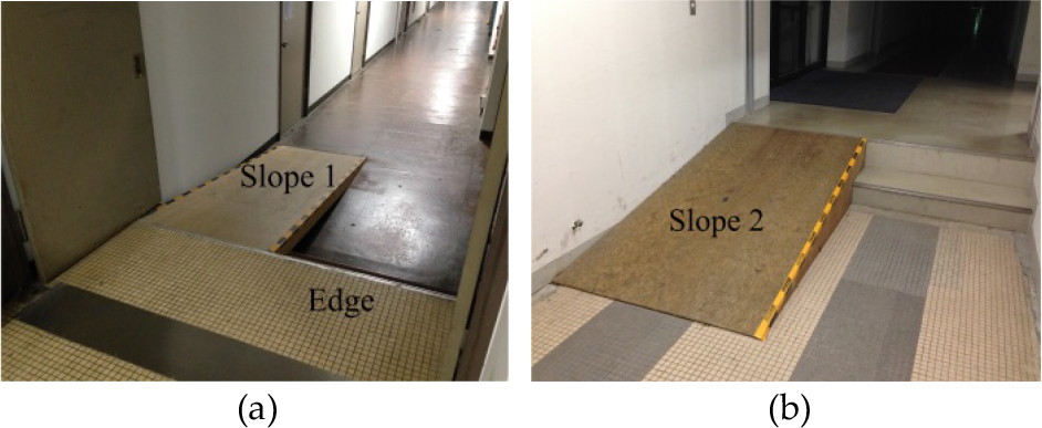
One downslope, one edge and one upslope

5.2 Experimental raw data

Figure 18 is plotted by utilizing the raw horizontal scanned data that are registered by the dead reckoning robot trajectory. The scanned data are severely corrupted because of the unbounded accumulating error of the dead reckoning pose. Notice that the data scanned from Slope 2 are very noisy considering the small shift of the robot during the scanning on the Slope 2; this is mainly due to the inclined surface of Slope 2 and rough ground in front of it. Figure 19 shows similar results for registered raw vertical scanned data. The area of Slope 2 can be easily found out while the area of Slope 1 is covered by the data scanned from the ground because of the huge reckoning error when robot returned to the initial position.

Figure 18.

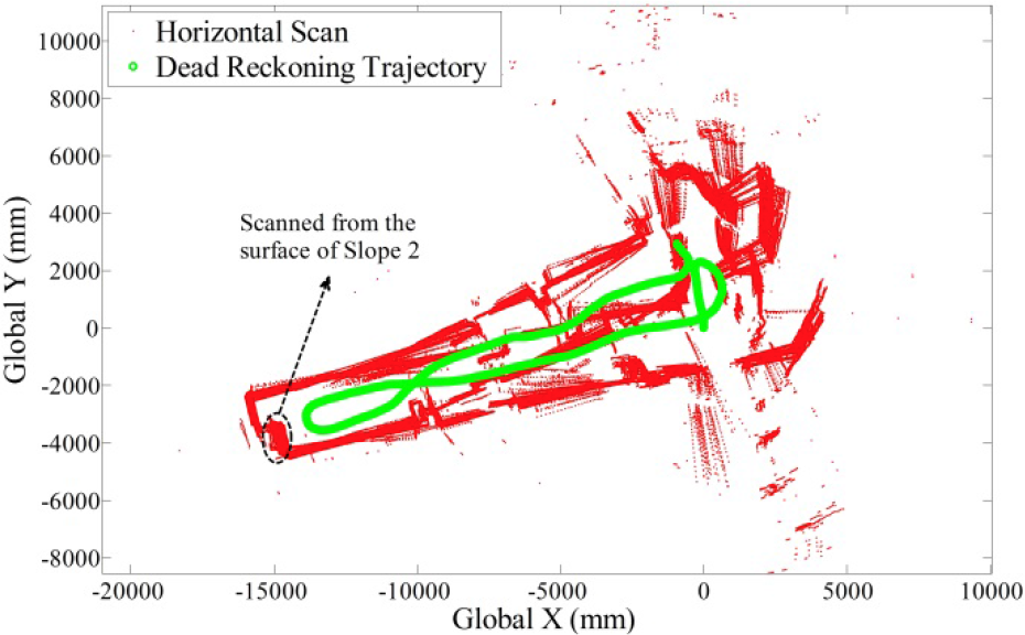
Horizontal scan registered by dead reckoning trajectory

Figure 19.

Vertical scan registered by dead reckoning trajectory

5.3 EKF-SLAM results

Figure 20 shows the EKF-SLAM result when the robot finished the vertical scanning on Slope 2 and turned back toward to the original position. Comparing with the one reckoned by odometer, the tracjctory has been obviously corrected, but it still has a certain amount of residual error which can be observed through the latest detected features in the left part of the figure.

Figure 20.

EKF-SLAM result in the halfway of the whole experiment

The final 2D EKF-SLAM result is shown in Figure 21 The features in the left part of the figure have been well corrected after the robot returned to the original position and re-observed the previous features Overall this 2D map gives a good top view of the environment.

Figure 21.

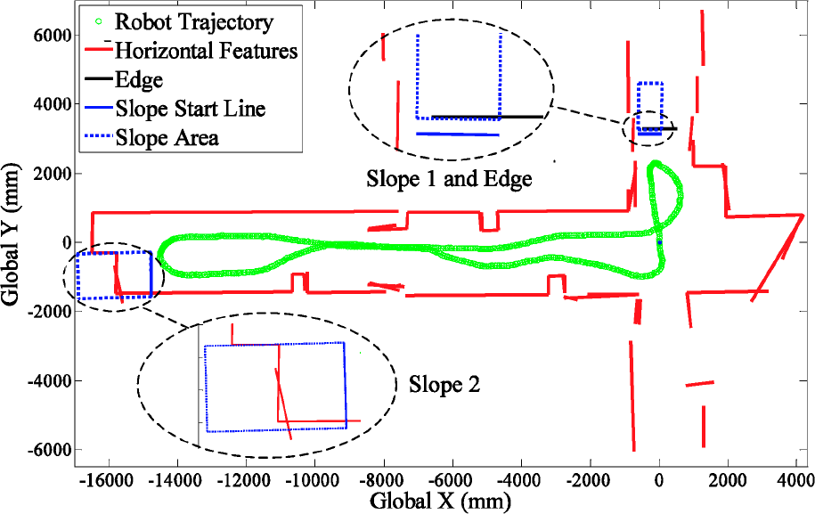
Final EKF-SLAM result with detected edge and slopes

However as shown in Figure 21 an unexpected small crack can be found between the start line of Slope 1 and the edge Since the slope start line is extracted from the intersection points of the line segment scanned from the slope and the ground line, this error is supposed to be mainly caused by the discontinuity between Slope 1 and the ground, as shown in Figure 22 As for Slope 2 a noisy horizontal line segment scanned from the slope's surface is recorded; this is mainly due to the imperfect flat ground When the LRF1 scans on the inclined surface of Slope 2 the noise can easily be aggravated when the robot moves on the tile covered ground and vibrates slightly some indication of this can be found in the scanned data pictured in Figure 18 The slightly overestimated width of the Slope 2 can be explained by the same reason.

Figure 22.

Discontinuity of the slope 1 with the ground

To verify the validity of the proposed algorithm all the vital parameters of edge and slope that are estimated by the EKF-SLAM are compared with the reference value to calculate the error as follows:

$Error=EKF\_result-Reference.$

(49)

It is noted that the reference values cannot be exactly true since they are measured by the author. The error of reference may be bigger than expected especially the reference of slope distance parameter ¶_s(1) which is an indirect measurement due to the discontinuity as shown in Figure 22.

The changes in all the errors with respect to the time (step) are shown in Figure 23, Figure 24 and Figure 25, respectively. The errors of the orthogonal angles are shown in Figure 23. Angle α_o(1) indicates the orientation of the edge line and start line of Slope 1 while α_o(2) only represents the angular parameter of the start line of slope 2. Both angles are varying and corrected during the robot motion. Figure 24 shows the errors of distance parameters ¶_e, ¶_s(1), and ¶_s(2), which correspond to the edge, slope 1 and slope 2, respectively. The errors of α_o(2) and ¶_s(2) diminish after step 460 when the robot moves towards the original position and re-observes the previous features. As for the gradient of the slopes, each of them is updated by an independent EKF so that they are corrected only when the corresponding slope is under observation, as shown in Figure 25.

Figure 23.

Error of orthogonal angles

Figure 24.

Error of distances parameters

Figure 25.

Error of slope angle

As the final SLAM result, the residual error of the orthogonal angle is mainly introduced by the error of local orthogonal angle estimation. The residual error is small but still slightly affects the orientation of the slope and edge. It can be found in the left bottom inset of Figure 21. The accuracy of distance parameter of slope and edge is mainly determined by the accuracy of orthogonal angle and the scanned slope line segment that were extracted in the vertical scan. Considering the size of the explored environment, the residual errors of distance parameters are acceptable. Based on the distance parameter and corresponding orthogonal angle, the location of slope and edge can be determined in 2D map and easy for consultation. The error of the slope gradient is free from the localization error and is mostly introduced by the error of scanned slope line segment and local orthogonal angle estimation. The estimated slope gradients are accurate enough for the robot to discover whether the slope is traversable.

5.4 Optional prediction results

To verify the efficiency of the optional prediction model, the error of the predicted transformation of the robot at each step should be presented. However, it is difficult to find the exact value of the robot pose transformation between two successive steps. Thus, the robot trajectory of the EKF-SLAM is adopted as the reference route and the transformation between the two steps can be calculated. The error can then be calculated as follows:

$Error=Prediction\_Trans.-EKF\_Trans.$

(50)

The optional prediction is executed in this EKF-SLAM, and out of a total of 700 steps, the ICP-based prediction is adopted in 174 steps while the remaining 526 steps adopt dead reckoning-based prediction.

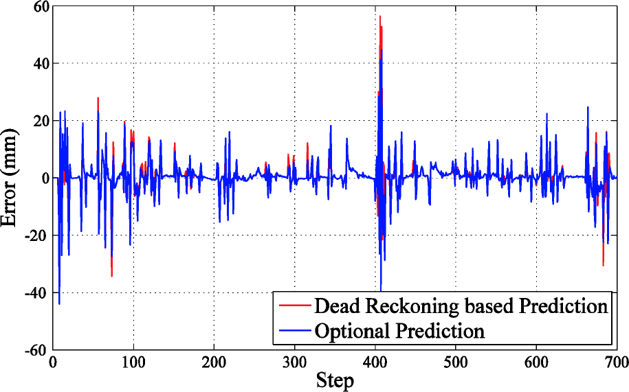
The pose transformation is composed of translation and rotation. The translational error is usually small since the robot cannot move at a high speed due to security considerations. Figure 26 and Figure 27 show plots of translational errors along X_R direction and Y_R direction at each step, respectively. Overall, the error along the Y_R is bigger than errors along X_R since the robot was moving forward instead of turning most of the time. However, no big difference can be found between the errors of two prediction models. Compared with the translational error, the rotational error is more critical because it normally leads to a very big error when the range of scanned data increases, which may lead to the failure of features association. The fatal rotational errors are substantially reduced by optional prediction, as shown in Figure 28.

Figure 26.

Comparison of translational error along X_R

Figure 27.

Comparison of translational error along Y_R

Figure 28.

Comparison of rotational errors

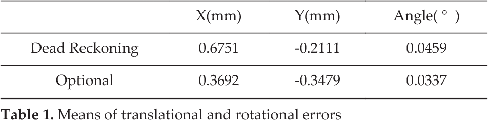
The statistical results of the error properties are listed in Table 1 and Table 2. All the means of errors listed in Table 1 are close to zero. Table 2 lists out the standard deviation of errors which can act as the judgment of performance between two prediction models. Optional prediction shows slightly bad results in translation. It is usually due to the scan error caused by LRF itself and slight vibration when the robot moving on the tiled floor. However, the translational distance between each step is usually over 50mm, thus these differences between two prediction models can be neglected. On the contrary, optional prediction gives a superior performance in the rotational error correction by reducing the rotational error over 32.7 percent. Since it makes the prediction more accurate, the feature association of EKF-SLAM will therefore be more robust.

Table 1.

Means of translational and rotational errors

	X(mm)	Y(mm)	Angle(°)
Dead Reckoning	0.6751	-0.2111	0.0459
Optional	0.3692	-0.3479	0.0337

Table 2.

Standard deviations of translational and rotational errors

	X(mm)	Y(mm)	Angle(°)
Dead Reckoning	6.0679	10.5175	1.1434
Optional	6.6889	11.2768	0.7687

5.5 Computational cost

It is well-known that the computational cost of EKF-SLAM is O(n²) per step where n is the number of stored feature [10]. The difference between the 3D version and 2D version is that the 3D feature has three parameters while 2D feature only has two parameters. Because of the quadratic form, 3D EKF-SLAM requires 2.25 times computational cost per step as much as 2D EKF-SLAM when they have the same feature number. Another extra computational cost of 3D SLAM comes from the feature extraction. Constrained plane and line segment are the preferred features of 3D SLAM [20] and 2D SLAM to represent structured indoor environment. The extraction of constrained plane from spatial point cloud requires much more computational cost than the line segment, which is extracted from fewer planar points.

Figure 29 shows the computational time of the proposed 2D algorithm at each step during the experiment. Overall, the time cost of each step is low. But it keeps increasing, however, along the experiment process because more and more features are detected and added into EKF-SLAM.

Figure 29.

Computational time of each step

In general, the step that adopts ICP-based prediction model requires higher computational cost than the step that adopts dead reckoning-based prediction. Obviously, the application of optional prediction successfully reduces the computational cost by selecting the appropriate prediction model. A few heavy costs, which require much higher computational time than the neighbouring steps, can be found. This is because the bad dead reckoning results require more iterations of ICP to compensate for the errors, especially when the rotational error is huge.

6. Conclusion and future work

In this study, a computationally inexpensive algorithm has been proposed to detect the slope and edge in a structured indoor environment. This algorithm is mainly composed of 2D line segment-based EKF-SLAM and orthogonal assumption. Instead of introducing an additional mechanism to rotate LRF to get 3D points clouds, a vertically fixed LRF framework has been adopted to enable the robot to fulfil the horizontal scan and vertical scan. Also, an optional prediction model has been proposed to select the suitable model from dead reckoning-based prediction and ICP-based prediction, which saves the computational cost and ensures the robustness of the prediction result. An experiment was conducted in a real indoor environment where there are edge, downslope, and upslope features The satisfactory results and analysis verify the validity of the proposed methods.

There are two main improvements that can be conducted in the future First, considering the rotational error of the prediction error, a metric-based ICP is usually reported to give a better solution than the traditional ICP Thus, some other variants of ICP can be compared and introduced to achieve better results Second, using a single vertical scan plane to monitor the ground is still risky for navigation The robot may fall from the edge which is nearly parallel to the robot displacement orientation and it is difficult to detect Additional cheaper sensors such as sonar can be introduced to monitor two sides of the robot to guarantee its safety.