Autonomous Navigation with Constrained Consistency for C-Ranger

Abstract

Autonomous underwater vehicles (AUVs) have become the most widely used tools for undertaking complex exploration tasks in marine environments. Their synthetic ability to carry out localization autonomously and build an environmental map concurrently, in other words, simultaneous localization and mapping (SLAM), are considered to be pivotal requirements for AUVs to have truly autonomous navigation. However, the consistency problem of the SLAM system has been greatly ignored during the past decades. In this paper, a consistency constrained extended Kalman filter (EKF) SLAM algorithm, applying the idea of local consistency, is proposed and applied to the autonomous navigation of the C-Ranger AUV, which is developed as our experimental platform. The concept of local consistency (LC) is introduced after an explicit theoretical derivation of the EKF-SLAM system. Then, we present a locally consistency-constrained EKF-SLAM design, LC-EKF, in which the landmark estimates used for linearization are fixed at the beginning of each local time period, rather than evaluated at the latest landmark estimates. Finally, our proposed LC-EKF algorithm is experimentally verified, both in simulations and sea trials. The experimental results show that the LC-EKF performs well with regard to consistency, accuracy and computational efficiency.

1. Introduction

Since the first relevant equation was put forward, simultaneous localization and mapping (SLAM), which is one of the key issues that need to be addressed for truly autonomous vehicles probing an unknown environment, has drawn tremendous attention in the realm of mobile robotics. Roughly speaking, SLAM can be categorized according to the means of map representation and the algorithms of its estimation technique. The well-known approaches of describing environmental maps are the feature-based method, the grid-based method, and the topological method. In addition, substantial estimation algorithms have been introduced to solve the SLAM issue, for instance, the extended Kalman filter (EKF) [1], the Extended Information Filter (EIF) [2], the unscented Kalman filter (UKF) [3], FastSLAM [4] and many other variants. However, EKF is the most common choice among the aforementioned algorithms, because it can be easily implemented, especially with lower computational complexity. Essentially speaking, EKF is a state filter or estimator. Therefore, consistency evaluation is essential for checking a filter design and evaluating its optimality.

Ever more appealing developments have been made in addressing the SLAM problem during the past decades. However, a large proportion of the attention has been devoted to handling the problems of computational complexity [5, 6], loop closing [7] and data association [8]. Another fundamental problem, of crucial importance, the consistency issue, has been greatly ignored and has only started to receive much attention, recently. The work by Julier and Uhlmann [9] pointed out for the first time that the SLAM algorithm inevitably obtains an inconsistent environment map by analysing a special case (namely, an immobile vehicle without process noise), as well as the general case of a mobile vehicle with process noise. Castellanos et al. [10] demonstrated that the EKF-SLAM state filter becomes inconsistent because of the linearization error and proposed a consistency-improved robocentric mapping approach. Bailey et al. [11] checked a large amount of inconsistent situations for EKF-SLAM and reached the conclusion that the uncertainty of the vehicle's orientation is the core reason for filter inconsistency. Later, theoretical analyses and experimental results presented by Huang and Dissanayake [12] also validated the corresponding conclusions reached by Bailey et al. and showed that the constrained Jacobians (i.e., Lemma 3.8 in reference [12]) could satisfy the prerequisite of filter consistency.

Technically speaking, the referenced works presented numerous inconsistent symptoms in EKF-SLAM, but did not reveal the deeper reasons for the filter inconsistency. Recently, the consistency problem of the EKF-SLAM was researched, based on an observability analysis, by Guoquan Huang et al. [13, 14] and a novel EKF-SLAM algorithm, based on the first estimates Jacobian (FEJ) was put forward to ameliorate the filter consistency. FEJ-EKF has been proved to have better consistency, compared with the standard EKF. However, the landmark estimates used for the linearization in FEJ-EKF are fixed after the first time within the global observation time and never updated. The weakness of FEJ-EKF is obvious: if the landmark estimates are inaccurate (this is a common situation), the resulting linearization errors will increase with them. To overcome this problem, we try to explore the consistency issue of EKF-SLAM in the local time period, delimited by the system order, rather than in the global time like the FEJ-EKF estimator. In this paper, a consistency constrained EKF-SLAM model based on the idea of local consistency is proposed and applied for the autonomous navigation of the C-Ranger AUV, which is developed as our experimental platform. The main contributions of this paper are as follows:

• 1)

  On the theoretical basis of local observability, we introduce the concept of local consistency, which is useful for the consistency analysis of the EKF-SLAM system in the local period;

  2)

  A novel LC-EKF estimator is proposed to improve the filter consistency of the EKF-based SLAM system efficiently by applying the methodology of local consistency.

  3)

  Sea trials on our own test platform, C-Ranger AUV are carried out to evaluate the performance of the LC-EKF. We also adopt the process of sensor data updating into the LC-EKF estimator for the purpose of improving performance.

  The remainder of this work is structured as follows: section 2 briefly restates the basic theory of the standard EKF-SLAM. In section 3, we introduce the concept of local consistency and then propose the LC-EKF estimator to improve the filter consistency in EKF-SLAM systems. Section 4 presents the general framework of our test platform, the C-Ranger AUV, as well as the on-board sensors installed on the C-Ranger. In Section 5, a set of experimental comparisons using simulations and our own datasets are carried out, while we also discuss the corresponding experimental results. Lastly, section 6 sketches out the crucial conclusions of this work.

  2. Restatement of standard EKF-SLAM algorithm

  As a recursive solution to the SLAM problem, the EKF model estimates the system state by minimizing the mean of the square error [15]. In this section, we briefly restate the state vector, the process model and prediction stage, the measurement model and update stage of the standard EKF-SLAM algorithm.

  2.1 State vector in EKF-SLAM

  In stochastic mapping, we can represent the system state at time step k by an augmented vector x _k including the vehicle pose vector x _{R k} and the position vector p _{L k} of a set of N_k landmarks in a known global reference frame and its covariance matrix P _k by correlations between the vehicle and landmarks:

  $$\begin{array}{l}{\mathrm{x}}_k={\left[\begin{array}{cc}{\mathrm{x}}_{R_k}^{\mathrm{T}}& {\mathrm{p}}_{L_k}^{\mathrm{T}}\end{array}\right]}^{\mathrm{T}}\\ ={\left[\begin{array}{cc}\begin{array}{cc}{\mathrm{p}}_{R_k}^{\mathrm{T}}& {\varphi }_{R_k}\end{array}& \begin{array}{ccc}{\left({\mathrm{p}}_{L_k}^1\right)}^{\mathrm{T}}& \cdots & {\left({\mathrm{p}}_{L_k}^{N_k}\right)}^{\mathrm{T}}\end{array}\end{array}\right]}^{\mathrm{T}}\\ ={\left[\begin{array}{cc}\begin{array}{ccc}{x}_{R_k}& y_{R_k}& {\varphi }_{R_k}\end{array}& \begin{array}{ccc}\begin{array}{cc}{x}_{L_k}^1& y_{L_k}^1\end{array}& \cdots & \begin{array}{cc}{x}_{L_k}^{N_k}& y_{L_k}^{N_k}\end{array}\end{array}\end{array}\right]}^{\mathrm{T}}\end{array}$$

  (1)
  $${\mathrm{P}}_k\text{=}\left[\begin{array}{cc}{\mathrm{P}}_{RR}& {\mathrm{P}}_{RL}\\ {\mathrm{P}}_{LR}& {\mathrm{P}}_{LL}\end{array}\right]$$

  (2)

  where the vehicle pose ${\mathrm{X}}_{R_k}={\left[{\mathrm{p}}_{R_k}^{\mathrm{T}}{\varphi }_{R_k}\right]}^{\mathrm{T}}$ includes the position ${\mathrm{p}}_{R_k}^{}$ and orientation ${\phi }_{R_k}$ of the mobile robot. If we suppose that the vehicle keeps running or moving in a plane, the vehicle position can be represented by the coordinates ${[x_{R_k}{y}_{R_k}]}^{\mathrm{T}}$ in the EN (east-north) reference frame, and the vehicle orientation is normally referred to as the heading, referenced to the north. ${\mathrm{p}}_{L_k}^j={[x_{L_k}^j{y}_{L_k}^j]}^{\mathrm{T}}$ denotes the position of the j ^th landmark.

  2.2 Process model and prediction stage for EKF-SLAM

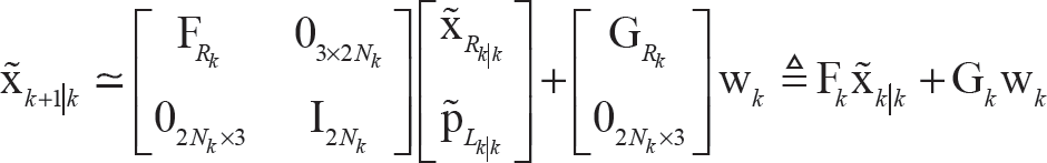
  The process model for the state prediction of the EKF-SLAM system is usually written as a first order non-linear formulation.

  $${\mathrm{x}}_{k+1}=\mathrm{f}\left({\mathrm{x}}_k\text{, }{\mathrm{u}}_k\right)+{\mathrm{w}}_k$$

  (3)

  where u _k is the known control input, w _k ∼N(0, Q_k) denotes the zero mean white Gaussian noise. The prediction formulation above Equation (3) can also be expressed by Equations 4–(6) in detail as:

  $${\widehat{\mathrm{p}}}_{R_{k+1|k}}={\widehat{\mathrm{p}}}_{R_{k|k}}+\text{C(}{\widehat{\varphi }}_{R_{k|k}}{)\Delta \widehat{\mathrm{p}}}_{R_{k+1|k}}$$

  (4)
  $${\widehat{\varphi }}_{R_{k+1|k}}={\widehat{\varphi }}_{R_{k|k}}+\text{Δ}{\widehat{\varphi }}_{R_{k+1|k}}$$

  (5)
  $${\widehat{\mathrm{p}}}_{L_{k+1|k}}={\widehat{\mathrm{p}}}_{L_{k|k}}$$

  (6)

  where C(·) presents the rotation matrix, the displacement ${\Delta \widehat{\mathrm{x}}}_{R_{k+1|k}}={\left[{\Delta \widehat{\mathrm{p}}}_{R_{k+1|k}}^{\mathrm{T}}\text{ Δ}{\widehat{\phi }}_{R_{k+1|k}}\right]}^{\mathrm{T}}$ between time step k and k+1 is estimated by odometry.

  Aside from the frequently used expression above, we can also express the EKF-SLAM system in its indirect form, i.e., the error-state space equation, where the state error $\tilde{\mathrm{x}}$ is the difference between the true state x and the estimated state $\widehat{\mathrm{x}}$ .

  $${\tilde{\mathrm{x}}}_{k+1|k}\simeq \left[\begin{array}{cc}{\mathrm{F}}_{R_k}& 0_{3\times 2N_k}\\ 0_{2N_k\times 3}& {\mathrm{I}}_{2N_k}\end{array}\right]\left[\begin{array}{c}{\tilde{\mathrm{x}}}_{R_{k|k}}\\ {\tilde{\mathrm{p}}}_{L_{k|k}}\end{array}\right]+\left[\begin{array}{c}{\mathrm{G}}_{R_k}\\ 0_{2N_k\times 3}\end{array}\right]{\mathrm{w}}_k\triangleq {\mathrm{F}}_k{\tilde{\mathrm{x}}}_{k|k}+{\mathrm{G}}_k{\mathrm{w}}_k$$

  (7)

  That is,

  $${\mathrm{F}}_k=\left[\begin{array}{cc}{\mathrm{F}}_{R_k}& 0_{3\times 2N_k}\\ 0_{2N_k\times 3}& {\mathrm{I}}_{2N_k}\end{array}\right]$$

  (8)
  $${\mathrm{G}}_k=\left[\begin{array}{c}{\mathrm{G}}_{R_k}\\ 0_{2N_k\times 3}\end{array}\right]$$

  (9)

  where the transition matrices ${\mathrm{F}}_{R_k}$ and ${\mathrm{G}}_{R_k}$ are as follows:

  $${\mathrm{F}}_{R_k}=\left[\begin{array}{cc}{\mathrm{I}}_2& \text{JC(}{\widehat{\varphi }}_{R_{k|k}}{)\Delta \widehat{\mathrm{p}}}_{R_{k+1|k}}\\ 0_{1\times 2}& 1\end{array}\right]=\left[\begin{array}{cc}{\mathrm{I}}_2& {\mathrm{J}(\widehat{\mathrm{p}}}_{R_{k+1|k}}-{\widehat{\mathrm{p}}}_{R_{k|k}}\text{)}\\ 0_{1\times 2}& 1\end{array}\right]$$

  (10)
  $${\mathrm{G}}_{R_k}=\left[\begin{array}{cc}\text{C(}{\widehat{\varphi }}_{R_{k|k}}\text{)}& 0_{2\times 1}\\ 0_{1\times 2}& 1\end{array}\right]$$

  (11)

  with $\mathrm{J}=\left[\begin{array}{cc}0& -1\\ 1& 0\end{array}\right]$ . Then the prediction covariance matrix will be:

  $${\mathrm{P}}_{k+1|k}={\mathrm{F}}_k{\mathrm{P}}_{k|k}{\mathrm{F}}_k{}^{\mathrm{T}}+{\mathrm{G}}_k{Q}_k{\mathrm{G}}_k{}^{\mathrm{T}}$$

  (12)
  2.3 Measurement model and update stage for EKF-SLAM

  The measurement model for the on-board sensor (e.g., sonar), observing the environmental features, can be expressed by the following nonlinear function h(·):

  $${\mathrm{z}}_k={\text{h(x}}_k\text{)}+{\mathrm{v}}_k$$

  (13)

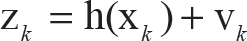
  where v _k ∼N(0, R_k) is the zero mean white Gaussian noise. The general relative position measurement can be written, in detail, as:

  $${\mathrm{z}}_k=\left[\begin{array}{c}{\mathrm{h}}_1{\text{(x}}_k\text{)}\\ {\mathrm{h}}_2{\text{(x}}_k\text{)}\end{array}\right]=\left[\begin{array}{c}\cos \text{(}{\varphi }_{R_k}{\text{)Δx}}_k^j+\sin \text{(}{\varphi }_{R_k}{\text{)Δy}}_k^j\\ -\sin \text{(}{\varphi }_{R_k}{\text{)Δx}}_k^j+\cos \text{(}{\varphi }_{R_k}{\text{)Δy}}_k^j\end{array}\right]$$

  (14)

  where ${\text{Δx}}_k^j=x_{L_k}^j-x_{R_k}$ , ${\text{Δy}}_k^j=y_{L_k}^j-y_{R_k}$ , $j=0,1,\mathrm{\dots },M_k$ . Similarly, the linearized error-state equation for measurement is:

  $${\tilde{\mathrm{z}}}_k\simeq \left[\begin{array}{cc}{\mathrm{H}}_{R_k}& {\mathrm{H}}_{L_k}\end{array}\right]\left[\begin{array}{c}{\tilde{\mathrm{x}}}_{R_{k|k-1}}\\ {\tilde{\mathrm{p}}}_{L_{k|k-1}}\end{array}\right]+{\mathrm{v}}_k\triangleq {\mathrm{H}}_k{\tilde{\mathrm{x}}}_{k|k-1}+{\mathrm{v}}_k$$

  (15)

  That is,

  $${\mathrm{H}}_k=\left[\begin{array}{cc}{\mathrm{H}}_{R_k}& {\mathrm{H}}_{L_k}\end{array}\right]$$

  (16)

  where ${\mathrm{H}}_{R_k}$ and ${\mathrm{H}}_{L_k}$ denote the Jacobian matrixes of h(·) for the vehicle pose and the landmark position:

  $${\mathrm{H}}_{R_k}=\text{(}\nabla {\mathrm{h}}_k{\text{)C}}^{\mathrm{T}}\text{(}{\widehat{\varphi }}_{R_{k|k-1}}\text{)}\left[\begin{array}{cc}-{\mathrm{I}}_2& -{\mathrm{J}(\widehat{\mathrm{p}}}_{L_{k|k-1}}-{\widehat{\mathrm{p}}}_{R_{k|k-1}}\text{)}\end{array}\right]$$

  (17)
  $${\mathrm{H}}_{L_k}=\text{(}\nabla {\mathrm{h}}_k{\text{)C}}^{\mathrm{T}}\text{(}{\widehat{\varphi }}_{R_{k|k-1}}\text{)}$$

  (18)

  where ∇h _k is the Jacobian matrix of h(·) calculated by the landmark's local position in the vehicle's coordinate system. Then, the innovation covariance matrix and the Kaiman gain can be evaluated as:

  $${\mathrm{S}}_k={\mathrm{H}}_k{\mathrm{P}}_{k|k-1}{\mathrm{H}}_k{}^{\mathrm{T}}+R_k$$

  (19)
  $${\mathrm{W}}_k={\mathrm{P}}_{k|k-1}{\mathrm{H}}_k{\left({\mathrm{S}}_k\right)}^{-1}$$

  (20)

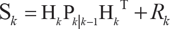
  Finally, the system state vector and its covariance matrix are updated as:

  $${\widehat{\mathrm{x}}}_{k|k}={\widehat{\mathrm{x}}}_{k|k-1}+{\mathrm{W}}_k{\upsilon }_k$$

  (21)
  $${\mathrm{P}}_{k|k}={\mathrm{P}}_{k|k-1}-{\mathrm{W}}_k{\mathrm{S}}_k{\mathrm{W}}_k{}^{\mathrm{T}}$$

  (22)

  where v _k presents the innovation sequence (also called the measurement residual).

3. Local consistency and LC-EKF estimator

Inevitably, the nonlinear functions in Equation (3) and (13) will cause errors, and the corresponding estimate results of the process and measurement model are not always accurate. In addition, the Jacobians in Equation (8), (9), (17) and (18) are evaluated using the latest estimated value of the system state vector, rather than its true value. Therefore, it is inevitable that the EKF system will confront the inconsistency problem. In this section, the consistency issue will be discussed in a local period for the classical EKF-SLAM system.

3.1 Local consistency based on observability analysis

Simply speaking, the typical EKF-SLAM system can be roughly classified into two sub-systems: the nonlinear SLAM sub-system and the linearized EKF sub-system.

3.1.1 Observability analysis for the nonlinear SLAM sub-system

Through the derivations of previous works [13, 14, 16], based on the important theory of observability rank condition [17], the observability matrix of the nonlinear SLAM sub-system with M _k observed landmarks at time step k can be given by ¹

$${\mathrm{O}}_k^{\mathrm{N}}\text{=span}\left[\begin{array}{cccc}\begin{array}{c}\begin{array}{c}s\varphi \\ \mathrm{c}\varphi \end{array}\\ \begin{array}{c}s\varphi \\ \mathrm{c}\varphi \\ ⋮\end{array}\\ \begin{array}{c}s\varphi \\ \mathrm{c}\varphi \end{array}\end{array}& \begin{array}{c}\begin{array}{c}-\mathrm{c}\varphi \\ s\varphi \end{array}\\ \begin{array}{c}-\mathrm{c}\varphi \\ \mathrm{s}\varphi \\ ⋮\end{array}\\ \begin{array}{c}-\mathrm{c}\varphi \\ s\varphi \end{array}\end{array}& \begin{array}{c}\begin{array}{c}-\mathrm{c}\varphi {\text{Δx}}_k^1-\mathrm{s}\varphi {\text{Δy}}_k^1{}_1\\ \mathrm{s}\varphi {\text{Δx}}_k^1-\mathrm{c}\varphi {\text{Δy}}_k^1\end{array}\\ \begin{array}{c}-\mathrm{c}\varphi {\text{Δx}}_k^2-\mathrm{s}\varphi {\text{Δy}}_k^2\\ \mathrm{s}\varphi {\text{Δx}}_k^2-\mathrm{c}\varphi {\text{Δy}}_k^2\\ ⋮\end{array}\\ \begin{array}{c}-\mathrm{c}\varphi {\text{Δx}}_k^{M_k}-\mathrm{s}\varphi {\text{Δy}}_k^{M_k}\\ \mathrm{s}\varphi {\text{Δx}}_k^{M_k}-\mathrm{c}\varphi {\text{Δy}}_k^{M_k}\end{array}\end{array}& \begin{array}{cccc}\begin{array}{c}\begin{array}{c}-\mathrm{s}\varphi \\ -\mathrm{c}\varphi \end{array}\\ \begin{array}{c}0\\ 0\\ ⋮\end{array}\\ \begin{array}{c}0\\ 0\end{array}\end{array}& \begin{array}{c}\begin{array}{c}\mathrm{c}\varphi \\ -\mathrm{s}\varphi \end{array}\\ \begin{array}{c}0\\ 0\\ ⋮\end{array}\\ \begin{array}{c}0\\ 0\end{array}\end{array}& \begin{array}{c}\begin{array}{c}0\\ 0\end{array}\\ \begin{array}{c}-\mathrm{s}\varphi \\ -\mathrm{c}\varphi \\ ⋮\end{array}\\ \begin{array}{c}0\\ 0\end{array}\end{array}& \begin{array}{ccc}\begin{array}{c}\begin{array}{c}0\\ 0\end{array}\\ \begin{array}{c}\mathrm{c}\varphi \\ -\mathrm{s}\varphi \\ ⋮\end{array}\\ \begin{array}{c}0\\ 0\end{array}\end{array}& \begin{array}{c}\begin{array}{c}0\\ 0\end{array}\\ \begin{array}{c}0\\ 0\\ ⋮\end{array}\\ \begin{array}{c}-\mathrm{s}\varphi \\ -\mathrm{c}\varphi \end{array}\end{array}& \begin{array}{c}\begin{array}{c}0\\ 0\end{array}\\ \begin{array}{c}0\\ 0\\ ⋮\end{array}\\ \begin{array}{c}\mathrm{c}\varphi \\ -\mathrm{s}\varphi \end{array}\end{array}\end{array}\end{array}\end{array}\right]$$

(23)

where sϕ and cϕ are the simplified modes of $\sin \text{(}{\phi }_{R_k}\text{)}$ and $\cos \text{(}{\phi }_{R_k}\text{)}$ . Examining the above matrix, we can see that the size of O _k ^N is 2M _k × (2M_k + 3). If the Gaussian elimination technique is applied to the observability matrix O _k ^N by row operations, we can obtain a reduced matrix in row echelon form where the number of nonzero rows is 2M _k . That is, the number of basic columns in O _k ^N is 2M _k . This number is defined as the rank of a matrix [18] which is an extremely important concept in the development of our work. Thus, we can obtain the following conclusion that:

Conclusion 1: The rank of the observability matrix for the general nonlinear SLAM sub-system, with M_k observed landmarks at time step k, is 2M_k.

3.1.2 Local observability analysis for the linearized EKF sub-system

Since the EKF system has been proven to be unobservable [16, 19], the local rather than the global observability matrix is chosen for the observability analysis for the EKF sub-system. The local observability matrix [20, 21] over the time period [k, k + n − 1] is defined as

$${\mathrm{O}}_k^{\mathrm{L}}=\left[\begin{array}{c}{\mathrm{H}}_k\\ {\mathrm{H}}_{k+1}{\mathrm{F}}_k\\ ⋮\\ {\mathrm{H}}_{k+n-1}{\mathrm{F}}_{k+n-2}\cdots {\mathrm{F}}_k\end{array}\right]$$

(24)

where n is the order of the linear time-varying (LTV) dynamical system, described by the error-state space Equations (7) and (15). According to reference [22], the system order n is defined as the number of state variables in the system, represented by state-space equations. Parameter n here is equal to the size of the state vector x _k in Equation (1). For example, the state vector is ${\mathrm{x}}_0={\left[\begin{array}{ccc}{x}_{R_0}& y_{R_0}& {\phi }_{R_0}\end{array}\right]}^{\mathrm{T}}$ at the initial time (i.e., k = 0) with no landmarks observed, so the EKF system is locally observable in the time interval [k, k + 2].

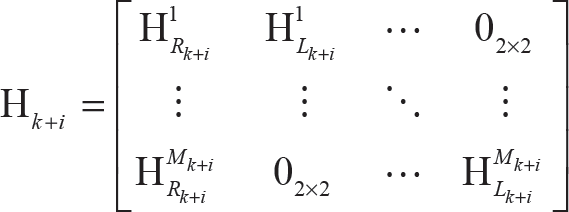
Suppose M_k+i landmarks are observed at time step k + i, where i = 0,1, …, n-1, then the measurement matrix can be written as

$${\mathrm{H}}_{k+i}=\left[\begin{array}{cc}\begin{array}{c}{\mathrm{H}}_{R_{k+i}}^1\\ ⋮\\ {\mathrm{H}}_{R_{k+i}}^{M_{k+i}}\end{array}& \begin{array}{ccc}{\mathrm{H}}_{L_{k+i}}^1& \cdots & 0_{2\times 2}\\ ⋮& \ddots & ⋮\\ 0_{2\times 2}& \cdots & {\mathrm{H}}_{L_{k+i}}^{M_{k+i}}\end{array}\end{array}\right]$$

(25)

Substituting the above equation into Equation (24), the observability matrix O _k ^L now becomes

$${\mathrm{O}}_k^{\mathrm{L}}=\left[\begin{array}{cc}\begin{array}{c}\begin{array}{c}{\mathrm{H}}_{R_k}^1\\ ⋮\\ {\mathrm{H}}_{R_k}^{M_k}\end{array}\\ \begin{array}{c}{\mathrm{H}}_{R_{k+1}}^1{\mathrm{F}}_{R_k}\\ ⋮\\ {\mathrm{H}}_{R_{k+1}}^{M_{k+1}}{\mathrm{F}}_{R_k}\end{array}\\ ⋮\\ \begin{array}{c}{\mathrm{H}}_{R_{k+n-1}}^1{\mathrm{F}}_{{\mathrm{R}}_{k+n-2}}\cdots {\mathrm{F}}_{R_k}\\ ⋮\\ {\mathrm{H}}_{R_{k+n-1}}^{M_{k+n-1}}{\mathrm{F}}_{{\mathrm{R}}_{k+n-2}}\cdots {\mathrm{F}}_{R_k}\end{array}\end{array}& \begin{array}{c}\begin{array}{ccc}{\mathrm{H}}_{L_k}^1& \cdots & 0_{2\times 2}\\ ⋮& \ddots & ⋮\\ 0_{2\times 2}& \cdots & {\mathrm{H}}_{L_k}^{M_k}\end{array}\\ \begin{array}{ccc}{\mathrm{H}}_{L_{k+1}}^1& \cdots & 0_{2\times 2}\\ ⋮& \ddots & ⋮\\ 0_{2\times 2}& \cdots & {\mathrm{H}}_{L_{k+1}}^{M_{k+1}}\end{array}\\ ⋮\\ \begin{array}{ccc}{\mathrm{H}}_{L_{k+n-1}}^1& \cdots & 0_{2\times 2}\\ ⋮& \ddots & ⋮\\ 0_{2\times 2}& \cdots & {\mathrm{H}}_{L_{k+n-1}}^{M_{k+n-1}}\end{array}\end{array}\end{array}\right]=\underset{{\mathrm{O}}_1}{\underbrace{\text{Diag}\left({\mathrm{H}}_{L_k}^1,\dots ,{\mathrm{H}}_{L_k}^{M_k},\cdots ,{\mathrm{H}}_{L_{k+n-1}}^1,\dots ,{\mathrm{H}}_{L_{k+n-1}}^{M_{k+n-1}}\right)}}\times \underset{{\mathrm{O}}_2}{\underbrace{\left[\begin{array}{cc}\begin{array}{c}\begin{array}{c}{({\mathrm{H}}_{L_k}^1)}^{-1}{\mathrm{H}}_{R_k}^1\\ ⋮\\ {({\mathrm{H}}_{L_k}^{M_k})}^{-1}{\mathrm{H}}_{R_k}^{M_k}\end{array}\\ \begin{array}{c}{({\mathrm{H}}_{L_{k+1}}^1)}^{-1}{\mathrm{H}}_{R_{k+1}}^1{\mathrm{F}}_{R_k}\\ ⋮\\ {({\mathrm{H}}_{L_{k+1}}^{M_{k+1}})}^{-1}{\mathrm{H}}_{R_{k+1}}^{M_{k+1}}{\mathrm{F}}_{R_k}\end{array}\\ ⋮\\ \begin{array}{c}{({\mathrm{H}}_{L_{k+n-1}}^1)}^{-1}{\mathrm{H}}_{R_{k+n-1}}^1{\mathrm{F}}_{{\mathrm{R}}_{k+n-2}}\cdots {\mathrm{F}}_{R_k}\\ ⋮\\ {({\mathrm{H}}_{L_{k+n-1}}^{M_{k+n-1}})}^{-1}{\mathrm{H}}_{R_{k+n-1}}^{M_{k+n-1}}{\mathrm{F}}_{{\mathrm{R}}_{k+n-2}}\cdots {\mathrm{F}}_{R_k}\end{array}\end{array}& \begin{array}{c}\begin{array}{ccc}{\mathrm{I}}_2{}^{}& \cdots & 0_{2\times 2}{}^{}\\ ⋮& \ddots & ⋮\\ 0_{2\times 2}{}^{}& \cdots & {\mathrm{I}}_2{}^{}\end{array}\\ \begin{array}{ccc}{\mathrm{I}}_2{}^{}& \cdots & 0_{2\times 2}{}^{}\\ ⋮& \ddots & ⋮\\ 0_{2\times 2}{}^{}& \cdots & {\mathrm{I}}_2{}^{}\end{array}\\ ⋮\\ \begin{array}{ccc}{\mathrm{I}}_2{}^{}& \cdots & 0_{2\times 2}{}^{}\\ ⋮& \ddots & ⋮\\ 0_{2\times 2}{}^{}& \cdots & {\mathrm{I}}_2{}^{}\end{array}\end{array}\end{array}\right]}}$$

(26)

1) Ideal EKF sub-system

The ideal EKF sub-system refers to a system where the true value of the state vector is known and thus

$${\mathrm{F}}_{R_{k+i}}=\left[\begin{array}{cc}{\mathrm{I}}_2& {\text{J(p}}_{R_{k+i+1}}-{\mathrm{p}}_{R_{k+i}}\text{)}\\ 0_{1\times 2}& 1\end{array}\right]$$

(27)

$${\mathrm{H}}_{R_{k+i}}^j=\left(\nabla {\mathrm{h}}_{k+i}\right){\mathrm{C}}^{\mathrm{T}}\left({\varphi }_{R_{k+i}}\right)\left[\begin{array}{cc}-{\mathrm{I}}_2& -\mathrm{J}\left({\mathrm{p}}_{L_{k+i}}^j-{\mathrm{p}}_{R_{k+i}}\right)\end{array}\right]$$

(28)

$${\mathrm{H}}_{L_{k+i}}^j=\left(\nabla {\mathrm{h}}_{k+i}\right){\mathrm{C}}^{\mathrm{T}}\left({\varphi }_{R_{k+i}}\right)$$

(29)

Then, we can obtain that

$${({\mathrm{H}}_{L_{k+i}}^j)}^{-1}{\mathrm{H}}_{R_{k+i}}^j{\mathrm{F}}_{{\mathrm{R}}_{k+i-1}}\cdots {\mathrm{F}}_{R_k}=\left[\begin{array}{cc}-{\mathrm{I}}_2& -\mathrm{J}\left({\mathrm{p}}_{L_{k+i}}^j-{\mathrm{p}}_{R_k}\right)\end{array}\right]$$

(30)

Substituting it into Equation (26), we can obtain ²

$${\mathrm{O}}_2^{\mathrm{I}}=\left[\begin{array}{ccc}\begin{array}{c}-{\mathrm{I}}_2\\ ⋮\\ -{\mathrm{I}}_2\end{array}& \begin{array}{c}-\mathrm{J}\left({\mathrm{p}}_{L_k}^1-{\mathrm{p}}_{R_k}\right)\\ ⋮\\ -\mathrm{J}\left({\mathrm{p}}_{L_k}^{M_0}-{\mathrm{p}}_{R_k}\right)\end{array}& \begin{array}{ccc}{\mathrm{I}}_2& \cdots & 0_{2\times 2}\\ ⋮& \ddots & ⋮\\ 0_{2\times 2}& \cdots & {\mathrm{I}}_2\end{array}\\ \begin{array}{c}-{\mathrm{I}}_2\\ ⋮\\ -{\mathrm{I}}_2\end{array}& \begin{array}{c}-\mathrm{J}\left({\mathrm{p}}_{L_{k+1}}^1-{\mathrm{p}}_{R_k}\right)\\ ⋮\\ -\mathrm{J}\left({\mathrm{p}}_{L_{k+1}}^{M_1}-{\mathrm{p}}_{R_k}\right)\end{array}& \begin{array}{ccc}{\mathrm{I}}_2& \cdots & 0_{2\times 2}\\ ⋮& \ddots & ⋮\\ 0_{2\times 2}& \cdots & {\mathrm{I}}_2\end{array}\\ ⋮& ⋮& ⋮\\ \begin{array}{c}-{\mathrm{I}}_2\\ ⋮\\ -{\mathrm{I}}_2\end{array}& \begin{array}{c}-\mathrm{J}\left({\mathrm{p}}_{L_{k+n-1}}^1-{\mathrm{p}}_{R_k}\right)\\ ⋮\\ -\mathrm{J}\left({\mathrm{p}}_{L_{k+n-1}}^{M_{n-1}}-{\mathrm{p}}_{R_k}\right)\end{array}& \begin{array}{ccc}{\mathrm{I}}_2& \cdots & 0_{2\times 2}\\ ⋮& \ddots & ⋮\\ 0_{2\times 2}& \cdots & {\mathrm{I}}_2\end{array}\end{array}\right]$$

(31)

Since the landmarks are static and their true values are known, the positions of the landmarks do not change with time, that is

$${\mathrm{p}}_{L_k}^j={\mathrm{p}}_{L_{k+1}}^j=\cdots ={\mathrm{p}}_{L_{k+i}}^j={\mathrm{p}}_L^j$$

(32)

So Equation (31) can be simplified as

$${\mathrm{O}}_2^{\mathrm{I}}=\left[\begin{array}{ccc}\begin{array}{c}-{\mathrm{I}}_2\\ ⋮\\ -{\mathrm{I}}_2\end{array}& \begin{array}{c}-\mathrm{J}\left({\mathrm{p}}_L^1-{\mathrm{p}}_{R_k}\right)\\ ⋮\\ -\mathrm{J}\left({\mathrm{p}}_L^{M_k}-{\mathrm{p}}_{R_k}\right)\end{array}& \begin{array}{ccc}{\mathrm{I}}_2& \cdots & 0_{2\times 2}\\ ⋮& \ddots & ⋮\\ 0_{2\times 2}& \cdots & {\mathrm{I}}_2\end{array}\\ \begin{array}{c}-{\mathrm{I}}_2\\ ⋮\\ -{\mathrm{I}}_2\end{array}& \begin{array}{c}-\mathrm{J}\left({\mathrm{p}}_L^1-{\mathrm{p}}_{R_k}\right)\\ ⋮\\ -\mathrm{J}\left({\mathrm{p}}_L^{M_{k+1}}-{\mathrm{p}}_{R_k}\right)\end{array}& \begin{array}{ccc}{\mathrm{I}}_2& \cdots & 0_{2\times 2}\\ ⋮& \ddots & ⋮\\ 0_{2\times 2}& \cdots & {\mathrm{I}}_2\end{array}\\ ⋮& ⋮& ⋮\\ \begin{array}{c}-{\mathrm{I}}_2\\ ⋮\\ -{\mathrm{I}}_2\end{array}& \begin{array}{c}-\mathrm{J}\left({\mathrm{p}}_L^1-{\mathrm{p}}_{R_k}\right)\\ ⋮\\ -\mathrm{J}\left({\mathrm{p}}_L^{M_{k+n-1}}-{\mathrm{p}}_{R_k}\right)\end{array}& \begin{array}{ccc}{\mathrm{I}}_2& \cdots & 0_{2\times 2}\\ ⋮& \ddots & ⋮\\ 0_{2\times 2}& \cdots & {\mathrm{I}}_2\end{array}\end{array}\right]$$

(33)

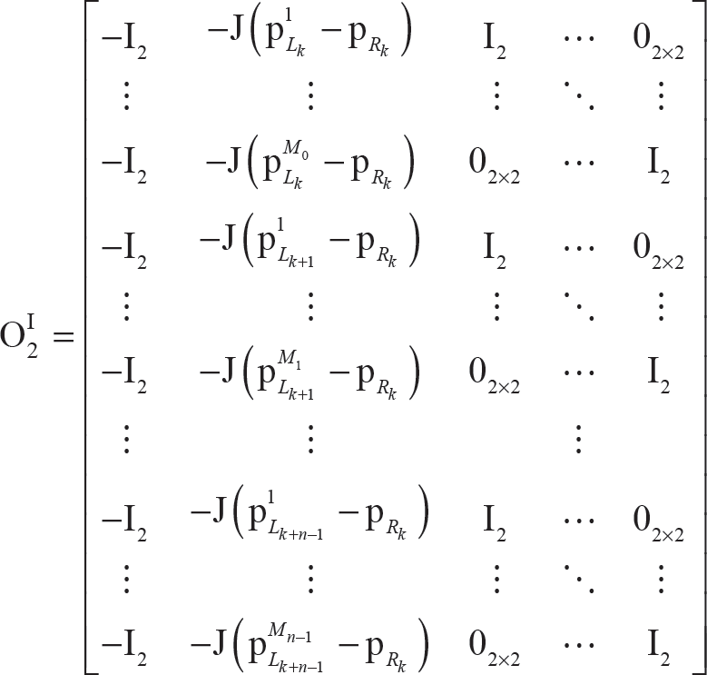
Since O₂^I is composed of n repetitive block rows, which can be described as:

$$o_{k+i}=\left[\begin{array}{ccc}\begin{array}{c}-{\mathrm{I}}_2\\ ⋮\\ -{\mathrm{I}}_2\end{array}& \begin{array}{c}-\mathrm{J}\left({\mathrm{p}}_L^1-{\mathrm{p}}_{R_k}\right)\\ ⋮\\ -\mathrm{J}\left({\mathrm{p}}_L^{M_{k+i}}-{\mathrm{p}}_{R_k}\right)\end{array}& \begin{array}{ccc}{\mathrm{I}}_2& \cdots & 0_{2\times 2}\\ ⋮& \ddots & ⋮\\ 0_{2\times 2}& \cdots & {\mathrm{I}}_2\end{array}\end{array}\right]$$

(34)

where i = 0,1, …, n − 1, and the size of each block row O_k+i is 2M_k+i X (2M_k+i + 3). That is,

$${\mathrm{O}}_2^{\mathrm{I}}=\left[\begin{array}{c}{o}_k\\ o_{k+1}\\ ⋮\\ o_{k+i}\\ ⋮\\ o_{k+n-1}\end{array}\right]$$

(35)

The elements of o_k+1, ···, o_k+n-1 can be converted to zero by the Gaussian elimination, as o_k+1, ···, o_k+n-1 ⊆ o _k . There are 2M_k nonzero rows in o_k, thus the rank of O₂^I is 2M_k. Therefore, we can reach the following conclusion that:

Conclusion 2: The rank of the observability matrix over the local time period [k, k + n − 1]for the ideal EKF sub-system, with M_k observed landmarks at time step k, is 2M_k, if M_k+1, ···, M_k+n-1 ≤ M _k .

We can see the rank of the observability matrix for the ideal EKF sub-system is equal to the nonlinear SLAM sub-system over the local time period, namely, they have the same observability property.

2) Standard EKF sub-system

For the standard EKF sub-system, Jacobian matrices are calculated using the latest estimated state, and thus

$${\mathrm{F}}_{R_{k+i}}=\left[\begin{array}{cc}{\mathrm{I}}_2& \mathrm{J}\left({\widehat{\mathrm{p}}}_{R_{k+i+1|k+i}}-{\widehat{\mathrm{p}}}_{R_{k+i|k+i}}\right)\\ 0_{1\times 2}& 1\end{array}\right]$$

(36)

$${\mathrm{H}}_{R_{k+i}}^j=\left(\nabla {\mathrm{h}}_{k+i}\right){\mathrm{C}}^{\mathrm{T}}\left({\widehat{\varphi }}_{R_{k+i|k+i-1}}\right)\left[\begin{array}{cc}-{\mathrm{I}}_2& -\mathrm{J}\left({\widehat{\mathrm{p}}}_{L_{k+i|k+i-1}}^j-{\widehat{\mathrm{p}}}_{R_{k+i|k+i-1}}\right)\end{array}\right]$$

(37)

$${\mathrm{H}}_{L_{k+i}}^j=\left(\nabla {\mathrm{h}}_{k+i}\right){\mathrm{C}}^{\mathrm{T}}\left({\widehat{\varphi }}_{R_{k+i|k+i-1}}\right)$$

(38)

Furthermore, we can also derive a formula analogous to Equation (30) as

$$\begin{array}{l}{\left({\mathrm{H}}_{L_{k+i}}^j\right)}^{-1}{\mathrm{H}}_{R_{k+i}}^j{\mathrm{F}}_{{\mathrm{R}}_{k+i-1}}\cdots {\mathrm{F}}_{R_k}\\ \text{=}\left[-{\mathrm{I}}_2-{\mathrm{J}(\widehat{\mathrm{p}}}_{L_{k+i|k+i-1}}^j-{\widehat{\mathrm{p}}}_{R_{k|k}}-{\displaystyle {\sum }_{l=k}^{k+i-2}({\widehat{\mathrm{p}}}_{R_{l+1|l+1}}-{\widehat{\mathrm{p}}}_{R_{l+1|l}})}\text{)}\right]\end{array}$$

(39)

Substituting it into Equation (26), we can obtain that

$${\mathrm{O}}_2^{\mathrm{S}}\text{=}\left[\begin{array}{ccccc}-{\mathrm{I}}_2& -\mathrm{J}({\widehat{\mathrm{p}}}_{L_{k|k-1}}^1-{\widehat{\mathrm{p}}}_{R_{k|k-1}})& {\mathrm{I}}_2& \cdots & 0_{2\times 2}\\ ⋮& ⋮& ⋮& \ddots & ⋮\\ -{\mathrm{I}}_2& -\mathrm{J}({\widehat{\mathrm{p}}}_{L_{k|k-1}}^{M_k}-{\widehat{\mathrm{p}}}_{R_{k|k-1}})& 0_{2\times 2}& \cdots & {\mathrm{I}}_2\\ -{\mathrm{I}}_2& -\mathrm{J}({\widehat{\mathrm{p}}}_{L_{k+1|k}}^1-{\widehat{\mathrm{p}}}_{R_{k|k}})& {\mathrm{I}}_2& \cdots & 0_{2\times 2}\\ ⋮& ⋮& ⋮& \ddots & ⋮\\ -{\mathrm{I}}_2& -\mathrm{J}({\widehat{\mathrm{p}}}_{L_{k+1|k}}^{M_{k\text{+}1}}-{\widehat{\mathrm{p}}}_{R_{k|k}})& 0_{2\times 2}& \cdots & {\mathrm{I}}_2\\ -{\mathrm{I}}_2& -\mathrm{J}({\widehat{\mathrm{p}}}_{L_{k+2|k\text{+}1}}^1-{\widehat{\mathrm{p}}}_{R_{k|k}}-{(\widehat{\mathrm{p}}}_{R_{k\text{+}1|k\text{+}1}}-{\widehat{\mathrm{p}}}_{R_{k\text{+}1|k}}\text{)})& {\mathrm{I}}_2& \cdots & 0_{2\times 2}\\ ⋮& ⋮& ⋮& \ddots & ⋮\\ -{\mathrm{I}}_2& -\mathrm{J}({\widehat{\mathrm{p}}}_{L_{k+2|k\text{+}1}}^{M_{k\text{+}2}}-{\widehat{\mathrm{p}}}_{R_{k|k}}-{(\widehat{\mathrm{p}}}_{R_{k\text{+}1|k\text{+}1}}-{\widehat{\mathrm{p}}}_{R_{k\text{+}1|k}}\text{)})& 0_{2\times 2}& \cdots & {\mathrm{I}}_2\\ ⋮& ⋮& ⋮& ⋮& ⋮\\ -{\mathrm{I}}_2& -\mathrm{J}({\widehat{\mathrm{p}}}_{L_{k+n-1|k+n-2}}^1-{\widehat{\mathrm{p}}}_{R_{k|k}}-{\displaystyle {\sum }_{l=k}^{k+i-3}({\widehat{\mathrm{p}}}_{R_{l+1|l+1}}-{\widehat{\mathrm{p}}}_{R_{l+1|l}})})& {\mathrm{I}}_2& \cdots & 0_{2\times 2}\\ ⋮& ⋮& ⋮& \ddots & ⋮\\ -{\mathrm{I}}_2& -\mathrm{J}({\widehat{\mathrm{p}}}_{L_{k+n-1|k+n-2}}^{M_{k\text{+}n-1}}-{\widehat{\mathrm{p}}}_{R_{k|k}}-{\displaystyle {\sum }_{l=k}^{k+i-3}({\widehat{\mathrm{p}}}_{R_{l+1|l+1}}-{\widehat{\mathrm{p}}}_{R_{l+1|l}})})& 0_{2\times 2}& \cdots & {\mathrm{I}}_2\end{array}\right]$$

(40)

As the state estimates generally differ at different times, the following formulas are normally tenable:

$${\widehat{\mathrm{p}}}_{L_{k|k-1}}^j\ne {\widehat{\mathrm{p}}}_{L_{k+1|k}}^j\ne \cdots \ne {\widehat{\mathrm{p}}}_{L_{k+i|k+i-1}}^j$$

(41)

$${\widehat{\mathrm{p}}}_{R_{l+1|l+1}}-{\widehat{\mathrm{p}}}_{R_{l+1|l}}\ne 0_{2\times 1}$$

(42)

Therefore, variables in the third column of O₂^S are not equal for different rows. Thus, we have to perform the column operations for the Gaussian elimination. As only the first two columns of O₂^S, which comprise 2M_k + 3 columns, can be eliminated, the rank of O₂^S is 2M_k + 1. Then we can conclude that:

Conclusion 3: The rank of the observability matrix over the local time period [k, k + n − 1] for the standard EKF sub-system, with M_k observed landmarks at time step k, is 2M _k + 1, if M_k+1, ···, M_k+n-1 ≤ M _k .

We can see that the standard EKF sub-system is not identical to the rank of the observability matrix of the nonlinear SLAM sub-system, in other words, the observability properties of the two sub-systems are not the same.

3.2 Local Consistency and LC-EKF estimator

In the preceding section, we performed an observability analysis of the nonlinear SLAM sub-system and the linearized EKF sub-system with any number of landmarks. Specially, when the number of landmarks is just one, we can come to the same conclusions as those in work [13] and find the corresponding relationship between observability and consistency as follows:

• 1)

  The ideal EKF sub-system has the same observability properties as the nonlinear SLAM sub-system within the local time period [k, k + n −1], consequently, the ideal EKF-SLAM system is consistent.

  2)

  The standard EKF sub-system's observability matrix has a higher rank than that of the nonlinear SLAM subsystem over the local time period [k, k + n − 1], which makes the standard EKF-SLAM system inconsistent.

  The two corollaries above, as well as the three conclusions drawn in section 3.1, look similar to those presented in references [13, 14], but they are actually restricted to the local time period rather than the global one, used by Huang et al. We think our conclusions are precise, because the theoretical basis of all the derivations, namely the local observability matrix, is defined over the local time period [k, k + n − 1]. So it is necessary to introduce the concept of local consistency for the EKF-SLAM system.

  Definition: The EKF-SLAM system is “locally consistent” if the linearized EKF sub-system has the same observability properties as the nonlinear SLAM sub-system over the time period [k, k + n − 1], where n is the order of the system.

  The local consistency, thus defined, differs from the well-known complete consistency, for the latter, the statement in the definition must be true for all values of k. Therefore, a system can be locally consistent for certain time intervals but not completely consistent.

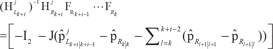
  As the extreme limit for FEJ-EKF is the usage of initial state estimates at the global time period for computing the filter Jacobians, we try to solve this problem in the local period by modifying the algorithm as follows:

  • 1)

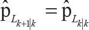
    If the Jacobian matrix in the EKF prediction stage is evaluated using the predicted value ${\widehat{\mathrm{p}}}_{R_{k+i|k+i-1}}$ rather than the updated value ${\widehat{\mathrm{p}}}_{R_{k+i|k+i}}$ as in the standard EKF, we can obtain

    $${\mathrm{F}}_{R_{k+i}}^{\text{'}}=\left[\begin{array}{cc}{\mathrm{I}}_2& \mathrm{J}\left({\widehat{\mathrm{p}}}_{R_{k+i+1|k+i}}-{\widehat{\mathrm{p}}}_{R_{k+i|k+i\text{-}1}}\right)\\ 0_{1\times 2}& 1\end{array}\right]$$

    (43)

  • 2)

    If the Jacobian matrices ${\mathrm{H}}_{R_k}^j,\cdots ,{\mathrm{H}}_{R_{k+n-1}}^j$ of the EKF update stage during every local time period [k, k + n − 1] are all evaluated using the landmark estimate ${\widehat{\mathrm{p}}}_{L_{k|k-1}}^j$ which is obtained at the first time instant of the local time period, we can obtain

    $$\begin{array}{l}{\mathrm{H}}_{k+i}^{\text{'}}=\left[\begin{array}{cc}{\mathrm{H}}_{R_{k+i}}^{\text{'}}& {\mathrm{H}}_{L_{k+i}}^{\text{'}}\end{array}\right]\\ =\left(\nabla {\mathrm{h}}_{k+i}\right){\mathrm{C}}^{\mathrm{T}}\left({\widehat{\varphi }}_{R_{k+i|k+i-1}}\right)\left[\begin{array}{ccc}-{\mathrm{I}}_2& -\mathrm{J}\left({\widehat{\mathrm{p}}}_{L_{k|k-1}}^j-{\widehat{\mathrm{p}}}_{R_{k+i|k+i-1}}\right)& -{\mathrm{I}}_2\end{array}\right]\end{array}$$

    (44)

  Then it is easy to obtain that

  $${({\mathrm{H}}_{L_{k+i}}^j)}^{-1}{\mathrm{H}}_{R_{k+i}}^j{\mathrm{F}}_{R_{k+i-1}}^{\text{'}}\cdots {\mathrm{F}}_{R_k}^{\text{'}}=\left[\begin{array}{cc}-{\mathrm{I}}_2& -\mathrm{J}\left({\widehat{\mathrm{p}}}_{L_{k|k-1}}^j-{\widehat{\mathrm{p}}}_{R_{k|k-1}}\right)\end{array}\right]{\mathrm{F}}_{R_{k+i}}^{\text{'}}$$

  (45)

  So, the observability matrix is

  $${\mathrm{O}}_2^{\text{'}}=\left[\begin{array}{ccc}\begin{array}{c}-{\mathrm{I}}_2\\ ⋮\\ -{\mathrm{I}}_2\end{array}& \begin{array}{c}-\mathrm{J}\left({\widehat{\mathrm{p}}}_{L_{k|k-1}}^1-{\widehat{\mathrm{p}}}_{R_{k|k-1}}\right)\\ ⋮\\ -\mathrm{J}\left({\widehat{\mathrm{p}}}_{L_{k|k-1}}^{M_k}-{\widehat{\mathrm{p}}}_{R_{k|k-1}}\right)\end{array}& \begin{array}{ccc}{\mathrm{I}}_2& \cdots & 0_{2\times 2}\\ ⋮& \ddots & ⋮\\ 0_{2\times 2}& \cdots & {\mathrm{I}}_2\end{array}\\ \begin{array}{c}-{\mathrm{I}}_2\\ ⋮\\ -{\mathrm{I}}_2\end{array}& \begin{array}{c}-\mathrm{J}\left({\mathrm{p}}_{L_{k|k-1}}^1-{\widehat{\mathrm{p}}}_{R_{k|k-1}}\right)\\ ⋮\\ -\mathrm{J}\left({\widehat{\mathrm{p}}}_{L_{k|k-1}}^{M_{k+1}}-{\widehat{\mathrm{p}}}_{R_{k|k-1}}\right)\end{array}& \begin{array}{ccc}{\mathrm{I}}_2& \cdots & 0_{2\times 2}\\ ⋮& \ddots & ⋮\\ 0_{2\times 2}& \cdots & {\mathrm{I}}_2\end{array}\\ ⋮& ⋮& ⋮\\ \begin{array}{c}-{\mathrm{I}}_2\\ ⋮\\ -{\mathrm{I}}_2\end{array}& \begin{array}{c}-\mathrm{J}\left({\widehat{\mathrm{p}}}_{L_{k|k-1}}^1-{\widehat{\mathrm{p}}}_{R_{k|k-1}}\right)\\ ⋮\\ -\mathrm{J}\left({\widehat{\mathrm{p}}}_{L_{k|k-1}}^{M_{k+n-1}}-{\widehat{\mathrm{p}}}_{R_{k|k-1}}\right)\end{array}& \begin{array}{ccc}{\mathrm{I}}_2& \cdots & 0_{2\times 2}\\ ⋮& \ddots & ⋮\\ 0_{2\times 2}& \cdots & {\mathrm{I}}_2\end{array}\end{array}\right]$$

  (46)

  If _k+1, ···, M_k+n-1 ≤ M _k , the rank of the observability matrix is 2M _k . Consequently, the above-modified system, which we call local consistency (LC) EKF SLAM, is locally consistent. The main process of the LC-EKF SLAM can be outlined by the following algorithm description.

  Algorithm 1 LC-EKF SLAM

  Inputs: initial estimates x _k and P _k Steps: 1. Initialize the filter. 2. Compute the system order n=size (x _k ). for t = k: k + n − 1 3. // EKF prediction stage while data from odometry sensor do Predict the system state x_k+1|k by Equation (4)–(6); Compute the prediction Jacobian F′ _k by substituting Equation (43) into (8); Predict the covariance matrix P_k+1|k by Equation (12) ; end while 4. // EKF update stage while data from measurement sensor do Data association; if the measurement is an existing landmark Compute the measurement Jacobian H' _k by Equation (44) ; Update the system state x_k+1|k and its covariance matrix P_k+1|k by Equation (19)–(22); end if if the measurement is a new landmark Augment the system state vector; end if end while 5. if = k Save ${\widehat{\mathrm{p}}}_{L_{k|k-1}}^j$ ; else if M_{k + 1} > M_k end if end for Outputs: estimates ${\widehat{\mathrm{x}}}_{t|t}$ and P_t|t 4. Overview of the C-Ranger AUV

  The C-Ranger vehicle was initially developed as a research platform for the testing and verification of various algorithms in underwater navigation. As detailed in our previous works [23–25], C-Ranger (Figure 1) is an open-frame-structure vehicle with the architecture of a control system, presented in Figure 2.

  
  Figure 1.

  C-Ranger AUV

  
  Figure 2.

  Control system of C-Ranger

  The C-Ranger is 1.6m long, 1.3m wide and 1.1m high. The total weight of the C-Ranger is about 206kg when working at full load. The maximum speed of the C-Ranger is close to 3 knots (1.5 m/s). Its continuous running time can reach eight hours when the C-Ranger travels at a speed of 1 knot and is fully charged.

  Numerous internal sensors, such as gyroscopes, digital compasses, pressure sensors and AHRS (Attitude and Heading Reference Systems), are installed on the C-Ranger. In addition, there are some external sensors–sonar, GPS and DVL (Doppler Velocity Log), for example.

  The basic sensors installed on the C-Ranger AUV are detailed in Table 1, as well as the newly added sensors, which enable the C-Ranger to perform the visual SLAM and multi-AUV SLAM.

  Table 1.

  Sensors installed on C-Ranger AUV

  

  Fundamental sensors	Variable	Update rate	Accuracy	Range
  Super SeaKing DST imaging sonar	Polar coordinate	0.05–0.2 Hz	15 mm (distance) 0.225 deg (angle)	0.4–300 m
  XW-GPS1000 GPS	XYZ position	1–20 Hz	1.1 m (CEP)	-
  NavQuest 600 DVL	Velocity	1–5 Hz	1% ± 1 mm/s	0.3–140 m
  Honeywell HMR3000 digital compass	Attitude	1–20 Hz	0.5 deg (RMS)	360 deg (heading) ± 40 deg (tilt)
  VG951D Gyroscope	Angular velocity	20 Hz	1 deg/h	60 deg/s
  Desert-star SSP-1 300PSIG Digital Pressure Sensor	Depth	0.25–16 Hz	0.1% of full scale	300 m
  UWM3000 Acoustic Modems	Communication	5 Kbps	<10-9	5000 m
  New sensors
  Gemini 720i Multibeam Imaging Sonar	Polar coordinate	5–30 Hz	8 mm (distance) 0.5 deg (angle)	0.2–120 m
  Innalabs® AHRS M2	Attitude	1–100 Hz	0.7 deg (heading) 0.4 deg (roll/pitch)	0–360 deg (heading) ±90 deg (pitch) ±180 deg (roll)
  Kongsberg Maritime OE14-376 (PAL) Colour Camera	Colour image	50 Hz	625 Line	3000m

5. Experiments and analysis

In this section, the following five algorithms are compared by using a large number of Monte Carlo simulations and our own sea trial dataset:

• (1)

  the ideal EKF SLAM

  (2)

  the standard EKF SLAM

  (3)

  the FEJ-EKF SLAM

  (4)

  the OC-EKF SLAM [26]

  (5)

  the proposed LC-EKF SLAM

  It should be noted that for the standard EKF SLAM, we relied on an existing Matlab implementation, developed by Tim Bailey, and the other three algorithms are all modified based on this. All the algorithms are executed in Matlab R2009a with 2.60GHz Pentium® Dual-Core CPU E5300 and 2GB RAM.

  5.1 Simulation Experiment

  The first test was carried out in a simulated environment, which allows comparison between the true states and the estimates to be made, as the true locations of the vehicle and landmarks are both available. In particular, all the simulations were carried out with known data association, so as to eliminate the influence of mismatching on the estimation of performance. As shown in Figure 3, there are 34 randomly generated point features and a vehicle trajectory with loop closure in a 200mx200m environment. The simulation parameters are detailed in Table 2.

  
  Figure 3.

  The simulation environment

  Table 2.

  Simulation parameters

  

  Parameter	Value
  Vehicle speed	5m/s
  Max scan range	30m
  Deadreckoning sampling time	0.025s
  Observation sampling time	0.125s
  Vehicle speed std dev	0.3m/s
  Steering angle std dev	3°
  Range observation std dev	0.1m
  Bearing observation std dev	1°

  To evaluate the performance of the estimators, 50 Monte Carlo tests are performed in the simulation scenario, where the vehicle fulfils five loops. The average Root Mean Square (RMS) errors of the vehicle pose are shown in Figure 4 to evaluate the accuracy of the five filters: the ideal EKF, the standard EKF, FEJ-EKF, OC-EKF and the LC-EKF. In addition, the average Consistency Index (CI) [5] of the vehicle pose presented in Figure 5 is used to evaluate the filters' consistency. It can be seen that our proposed LC-EKF algorithm performs better than the standard EKF and the FEJ-EKF, and has a performance comparable with the OC-EKF, pertaining to the accuracy and consistency.

  
  Figure 4.

  Mean RMS errors of the vehicle pose

  
  Figure 5.

  Mean consistency index (CI) of the vehicle pose

5.2 Sea Trial

5.2.1 SLAM for C-Ranger

Consider that in our current system, the C-Ranger always remains stable in the DOFs (degrees of freedom) of roll and pitch, the state vector of the C-Ranger can be presented by:

$${\mathrm{x}}_R^{}={\left[x_R{y}_R{z}_R{\varphi }_R{v}_x{v}_y{v}_z\right]}^{\mathrm{T}}$$

(47)

where [x_R y_R z_R ϕ _R ]^T denotes the 3-D coordinates and the heading of the C-Ranger in the global reference frame and [v_x v_y v_z]^T are the linear velocities in the vehicle reference frame.

The motion model of the C-Ranger moving at a constant velocity from time k-1 to k can be written as

$${\mathrm{x}}_{R_k}=\mathrm{f}\left({\mathrm{x}}_{R_{k-1}}\text{, }{\mathrm{u}}_k\right)+{\mathrm{w}}_k$$

(48)

$${\left[\begin{array}{l}{x}_R\\ y_R\\ z_R\\ {\varphi }_R\\ v_x\\ v_y\\ v_z\end{array}\right]}_k={\left[\begin{array}{c}{x}_R+\mathrm{\Delta }x\cos \text{(}{\varphi }_R\text{)}-\mathrm{\Delta }y\sin \text{(}{\varphi }_R\text{)}\\ y_R+\mathrm{\Delta }x\sin \text{(}{\varphi }_R\text{)}+\mathrm{\Delta }y\cos \text{(}{\varphi }_R\text{)}\\ z_R+\mathrm{\Delta }z\\ {\varphi }_R+w\mathrm{\Delta }\mathrm{T}\\ v_x+a_x\mathrm{\Delta }\mathrm{T}\\ v_y+a_y\mathrm{\Delta }\mathrm{T}\\ v_z+a_z\mathrm{\Delta }\mathrm{T}\end{array}\right]}_{k-1}+{\mathrm{w}}_k$$

(49)

with the displacements:

$$\begin{array}{c}\Delta x=v_x\Delta \mathrm{T}+\frac{1}{2}{a}_x{\left(\Delta \mathrm{T}\right)}^2\\ \Delta y=v_y\Delta \mathrm{T}+\frac{1}{2}{a}_y{\left(\Delta \mathrm{T}\right)}^2\\ \Delta z=v_z\Delta \mathrm{T}+\frac{1}{2}{a}_z{\left(\Delta \mathrm{T}\right)}^2\end{array}$$

(50)

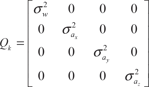
where the control input vector u _k = [w a_x a_y a_z]^T is composed of the angular velocity and the accelerations. ³ Furthermore, w _k denotes the white Gaussian control noise with a zero mean and covariance matrix Q_k:

$$Q_k=\left[\begin{array}{cccc}{\sigma }_w^2& 0& 0& 0\\ 0& {\sigma }_{a_x}^2& 0& 0\\ 0& 0& {\sigma }_{a_y}^2& 0\\ 0& 0& 0& {\sigma }_{a_z}^2\end{array}\right]$$

(51)

For the C-Ranger, using sonar as the observing sensor, the range-bearing measurement model can be written in the form ⁴

$$z_k^S=\left[\begin{array}{c}r\\ \psi \end{array}\right]=\left[\begin{array}{c}\sqrt{{\text{(}{x}_L-x_R\text{)}}^2+{\text{(}{y}_L-y_R\text{)}}^2}\\ {\tan }^{-1}\text{(}\frac{y_L-y_R}{x_L-x_R}\text{)}-{\varphi }_R\end{array}\right]+{\mathrm{v}}_k^S$$

(52)

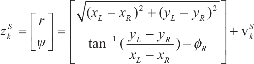
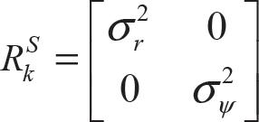
where v _k ^S denotes the white Gaussian measurement noise for sonar with zero mean and covariance matrix R _k ^S :

$$R_k^S=\left[\begin{array}{cc}{\sigma }_r^2& 0\\ 0& {\sigma }_{\psi }^2\end{array}\right]$$

(53)

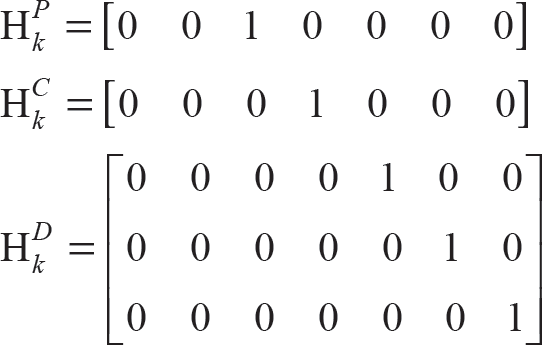
As described in Section 4, the C-Ranger is also equipped with many other sensors, which can supply direct observations of components in the state vector. For the pressure sensor, the digital compass and the DVL, the measurement models are linear, and their measurement matrix and measurement noise can be given as:

$$\begin{array}{l}{\mathrm{H}}_k^P=\left[0010000\right]\\ {\mathrm{H}}_k^C=\left[0001000\right]\\ {\mathrm{H}}_k^D=\left[\begin{array}{l}0000100\\ 0000010\\ 0000001\end{array}\right]\end{array}$$

(54)

$$\begin{array}{l}{R}_k^P={\sigma }_P^2\\ R_k^C={\sigma }_C^2\\ R_k^D=\left[\begin{array}{ccc}{\sigma }_{v_x}^2& 0& 0\\ 0& {\sigma }_{v_y}^2& 0\\ 0& 0& {\sigma }_{v_z}^2\end{array}\right]\end{array}$$

(55)

Substituting Equations (54) and (55) into Equations (19)–(22), the sensor data in the state vector can be updated. This process is called sensor data updating, which can make the sensor data more accurate before they are fed into the motion model of the C-Ranger.

5.2.2 Experimental results

We carried out the sea trial at Tuandao Bay, in Qingdao, China. Figure 6 demonstrates the experimental results integrated with the environmental satellite image. The magenta points denote the point features, extracted from the sonar data, which match well with landmarks in the real world.

Figure 6.

Results of the sea trial combined with the satellite image

A clear path comparison is presented in Figure 7, where the GPS trajectory (the cyan line) works as the ground truth for the comparison of the algorithms. It can be seen that the path deviation of our proposed LC-EKF relative to the GPS is smaller than that of the standard EKF and the FEJ-EKF. The LC-EKF's outperformance can also be confirmed by comparisons with RMS (Figure 8) and CI (Figure 9).

Figure 7.

Path comparison

Figure 8.

RMS errors of the vehicle pose

Figure 9.

CI of the vehicle pose

Moreover, the computational cost is used to evaluate the performance of the estimator. The standard EKF, FEJ-EKF and LC-EKF estimators are all based on the EKF-SLAM systems, and the essential differences between them are just their usage of state estimates to compute the Jacobian matrix at different time points. Therefore, the computational costs for the standard EKF, FEJ-EKF and LC-EKF estimators are almost the same. We only need to compare the proposed LC-EKF with the OC-EKF. The total cost of the CPU time for the LC-EKF is 131.5 seconds and that for the OC-EKF is about 1108.8 seconds. The detailed CPU time required for each timestep is shown in Figure 10. As the time cost of the LC-EKF is far less than that of the OC-EKF, the LC-EKF is more appropriate for real time application.

Figure 10.

CPU time for each timestep

6. Conclusion

In this paper a consistency constrained EKF-SLAM algorithm based on the idea of local consistency is proposed and applied for the autonomous navigation of our test platform, the C-Ranger AUV. The concept of local consistency is introduced after an explicit theoretical derivation of the EKF-SLAM system. Furthermore, we present a locally consistency-constrained EKF-SLAM design, LC-EKF, in which the landmark estimates used for linearization are fixed at the beginning of each local time period rather than evaluated at the latest landmark estimates. Finally, the experimental results of our simulation and real-world tests show that our proposed LC-EKF algorithm performs well with respect to consistency, accuracy and computational efficiency. With this improved algorithm, autonomous navigation systems can be extended to numerous engineering applications, such as autonomous underwater vehicles (AUV), unmanned land vehicles and unmanned aerospace vehicles (UAV).