A Robust Vision Module for Humanoid Robotic Ping-Pong Game

Abstract

Developing a vision module for a humanoid ping-pong game is challenging due to the spin and the non-linear rebound of the ping-pong ball. In this paper, we present a robust predictive vision module to overcome these problems. The hardware of the vision module is composed of two stereo camera pairs with each pair detecting the 3D positions of the ball on one half of the ping-pong table. The software of the vision module divides the trajectory of the ball into four parts and uses the perceived trajectory in the first part to predict the other parts. In particular, the software of the vision module uses an aerodynamic model to predict the trajectories of the ball in the air and uses a novel non-linear rebound model to predict the change of the ball's motion during rebound. The average prediction error of our vision module at the ball returning point is less than 50 mm - a value small enough for standard sized ping-pong rackets. Its average processing speed is 120fps. The precision and efficiency of our vision module enables two humanoid robots to play ping-pong continuously for more than 200 rounds.

1. Introduction

This paper presents a robust predictive vision module for a humanoid robotic ping-pong game. The robotic ping-pong game is a challenging task which was first introduced by John Billingsley in 1983 [1]. Several research teams developed robotic ping-pong players to join John's game [2–6]. These inspiring work triggered the study of robotic ping-pong players: some used non-humanoid mechanisms like DELTA robots and x-y robots [3, 6–13]. Some others used articulated robotic arms of five to seven degrees of freedom (DOFs) [2, 4, 5, 14–17]. Some like [18–20] and ours [21] used dual-arm or humanoid robots to play ping-pong. We use two humanoid robots to play ping-pong with each other.

Using two humanoid robots to play ping-pong using a standard sized ping-pong table is quite fascinating and attracts a lot of social attention. However, the precision and efficiency requirements of the vision module are quite critical: (1) Unlike non-humanoid robotic ping-pong players, of which most of the constraints are from mild kinematics, humanoid robots have an unfixed base and suffer from the curse of high DOFs. A large error in ball detection and prediction plus the accumulated error in control increases the risk of losing the ball during the game. In contrast, precise prediction will spare comparatively more tolerance for the accumulated control error. A humanoid robotic ping-pong game requires the vision module to be precise. (2) Unlike a human-robot ping-pong game where a human player may intentionally cater the robotic players during demonstration, two robots cannot cater each other by slowing down the ball motion intentionally, or else they may lose the ball. A ping-pong ball is always in high speed during a robot-robot ping-pong game. A humanoid robotic ping-pong game also requires the vision module to be efficient.

In this paper, we present a precise yet high-speed vision module for two humanoid robots playing a ping-pong game with each other. Our vision module uses stereo vision for ball trajectory detection and non-linear physical models for ball trajectory prediction. The hardware of the vision module is composed of two stereo camera pairs with each of them detecting the 3D positions of the ball at one half of the ping-pong table. The software of the vision module divides the trajectory of a ping-pong ball into four parts and uses the detected 3D positions in the first part of the trajectory to predict the other parts. The software of the module uses thresholding plus elliptic fitting to detect the 2D positions of the ball in the images of each camera and to reconstruct the 3D positions of the ball by stereo triangulation. It uses an aerodynamic model to predict the trajectories of the ball in the air and uses a newly proposed non-linear rebound model based on impulse momentum theorem to predict the change of the ball's motion during rebound. The hardware configuration plus the software development of the module exhibits high performance. Experiments show that our vision module performs better in trajectory prediction than a conventional Linear Weighted Regression (LWR) approach. Its average prediction error is less than 50 mm, a value small enough for standard ping-pong rackets. Our vision module has an efficient processing speed of 120 fps. It is precise, efficient and robust, and enables two humanoid robots to play a ping-pong game continuously for more than 200 rounds.

The organization of this paper is as follows. Section 2 reviews the related vision modules for a robotic ping-pong game. Section 3 presents the hardware aspect of our vision module like the configuration of cameras and the specification of the processing unit. It also presents the details of our humanoid robots. Section 4 discusses the software aspect of our vision module like the aerodynamic model, the non-linear rebound model, the ball detection algorithms and the ball prediction algorithms. Experiments and analysis are shown in section 5. Section 6 draws the conclusion.

2. Related Work

There are lots of vision modules for a robotic ping-pong game. We discuss them from two aspects: the hardware configuration, like camera number and camera types, and software development like detection and prediction algorithms, respectively.

2.1 Hardware Configuration

The requirements of high precision and high processing speed add lots of constraints to hardware configuration like camera number, camera location, camera resolution plus the frame rate of cameras and the configuration of the processing units.

The number of cameras used by the vision modules of ping-pong robots ranged from one to four or more. Much work [3, 7, 10, 11, 13] employed a single camera to detect the ping-pong ball. Using a single camera led to a high processing speed. However, it also resulted in a large detection error. Acosta et al. [7] and Peng et al. [10] made efforts to lower the detection error of single-camera vision modules by processing images that contained both the ball and its shadow. It was an interesting solution but depended heavily on the shadow and environment light. Some other work used binocular cameras [4–6, 8, 14, 15, 17, 22, 23] to improve perception precision. The resolution of these binocular cameras ranged from 232times232 to 2048times2048. Resolution is an important part of binocular cameras. For one thing, it is related to processing speed. Large resolution significantly lowers ball detection speed. For the other, it is related to the field of view (FOV). A camera with small resolution cannot see large scene with high precision. In order to find a balance between processing speed and precision, some of the developers used smaller ping-pong tables instead of standard ones [4–7]. Others used special cameras and processors [15, 22]. Four-camera based vision modules were presented by Andersson [24] and Lampert et al. [25] to improve perception precision. Andersson developed a four-camera vision module for a PUMA 260 ping-pong robot. The module used one pair of the cameras for short range perception of the rebound trajectory and the other pair of the cameras for long range perception of the trajectory before rebound. Lampert et al. developed an RTblob vision module which used four off-the-shelf cameras plus two standard personal computers to perform fast ping-pong ball detection. They claimed that their module was the most precise affordable module at that time. Like them, we use two stereo pairs to obtain the trajectories of the ping-pong ball. We divide the four cameras into two stereo pairs to perceive the two halftables, respectively. The division increases perception precision without reducing perception speed. We will discuss the details in Section 3.

Installation of the cameras is another point of the hardware configuration. Some work [3, 11, 13] used active cameras to track the ball. Active cameras were installed on the end-effectors or certain motor joints of the ping-pong robots. These cameras could be actively actuated to capture images of a small region of the ping-pong ball and to reduce the size of the captured images. However, active actuation blurred the captured images and lowered the precision of the vision modules. We therefore install four fixed cameras in extrinsic environment rather than actively attaching them to robot joints or end-effectors.

Besides camera number and camera location, camera resolution, camera frame rate and the configuration of the processing units play an important role in the perception performance of the vision modules. Here we presented the hardware configurations of some famous ping-pong robots' vision modules. In the early years, low resolution cameras and low speed processing units such as embedded microprocessor-based control boards were used. In Hashimoto's vision module [4], the resolution plus frame rate of cameras were 2048×1×100Hz, and the processing unit was a multi-microcomputer system composed of seven microprocessor boards, three of which used 32bit microprocessors and the other four used 16bit microprocessors. The speed reached up to 80ms or 12.5Hz. In Andersson's vision module [24], the resolution plus frame rate of cameras was 756times484times30Hz, and the processing unit was composed of two circuit boards, TRIAX and JIFFE for 2D and 3D data processing, respectively, and the processing speed is 32.2ms or 31Hz with image size 756times242. Later, integrated commercial high speed vision systems were adopted as vision modules. A commercial Quick Mag vision system was used in Matsushima's table tennis robot [8]. The system was capable of detecting the ball's 3D positions at 60Hz with size 640times416. Nakashima [15] used a commercial high speed stereo vision system which has a speed of 232times232 @ 900fps from Hamamatsu Photonics. Now, the most popular and affordable hardware configuration is to use high speed cameras with USB, CAMERALINK, Ethernet, GiGE or 1394 interface, image grab cards with the same interface, and a personal PC or workstation with or without GPU acceleration. The camera used in paper [14] had an image-grab speed of 640times480 @ 66Hz. A PC with a Linux operating system was used as the processing unit. However, the system was only able to perceive the ball at a low speed of 15Hz because of the bandwidth limit of USB1.1 on his computer. Paper [23] used IMPERX IPX-210 cameras with a camera link interface and an image capture card DALSA X64-CL. The processing unit was a HP workstation XW 8200. The resolution plus frame rate of the cameras was 640times480times110 fps. The binocular vision system in paper [17] used a similar hardware configuration. Two IMPERX(R) IPX-1M48-L cameras of 1000times600 @ 48Hz, an image grab card DALSA X64-CL-iPro and a personal PC with Intel(R) Core(TM)2 i5 CPU 2.6GHz and NVIDIA(R) GTS260 GPU were used to constitute the vision module. The vision module had a speed of 1000times600 @ 48Hz. Lampert et al.‘s vision module [25] used four Ethernet cameras named Prosilica GE640 @ 640times480times200fps and Intel PRO/1000 PT Quad Port gigabit Ethernet card. The processing unit was a Dell Precision T7400 workstation with two 3.4GHz Intel Dual-Core CPUs and a NVIDIA GeForce GTX 280 GPU graphics card. They claimed that their module was the most precise affordable module.

Paper [22] used two greyscale smart cameras @ 640times480times250fps. The two cameras were connected to a personal computer via Ethernet through a TCP/IP protocol. The processing speed reached up to 640times480times100Hz. In this paper, we used four 1394b cameras of 640×480×3ch × 200fps, two PCIe 1394b image grab cards and an ordinary PC as the processing unit. The hardware configuration plus the software resulted in a processing speed of 120 fps.

2.2 Software Development

The software aspect of the vision module is mainly about the development of detection and prediction algorithms.

Precise and fast ball detection is an important prerequisite of good prediction performance. Previous studies developed or borrowed many ball detection algorithms, e.g., binary contours for the soccer ball [26], background subtraction for the tennis ball [27], hough transform for the soccer ball [28], etc., to ensure precise and efficient detection of the ping-pong ball. For example, Nakashima et al. [15] used thresholding to binarize greyscale images and to find the contour of the ping-pong ball. They compute the centre of the ball by averaging the four outermost points on vertical and horizontal boundaries of the contour. Tian et al. [23] used a similar five-point method to detect the centre of the ball. The thresholding method was very fast. Unfortunately, it was not as precise. Modi et al. [14] used both binary contours and background subtraction to detect the ping-pong ball. They did not only compute the silhouette of the ball by thresholding but also computed the motion of the ball by differentiating sequential silhouettes. They took the motion as noises and removed them from the silhouettes to improve detection precision. How to get rid of the blurring noises caused by motion is a common problem in ping-pong ball detection algorithms. Like Modi, Zhang et al. [22] used background subtraction to detect the motion of the ping-pong ball. However, instead of taking the motion as noise, they used the motion of the ball as a detection feature. They combined the motion of the ball together with a method called the growth of sampled points (GSP) to recover its position. Liu et al. [17] solved the motion-blur problem by using a detection model which inherently encoded the motion of the ball. The detection model significantly improved the precision of their vision module. Zhang et al. [29] used an elliptic model to fit the blurred ball. They also got precise detection results since the elliptic fitting model encoded the motion of the ball as the detection model of Liu et al. [17]. Instead of a binary contour method and background subtraction method, Lampert et al. [25] used a linear shift invariant filter (LSI) [30], which was essentially like the gradient calculator in the first step of hough transform, to detect the silhouette of the ping-pong ball. Their filters were elliptic and they used GPU to ensure high processing speed. Although it was not explicitly claimed, Andersson [24] employed a similar gradient-based filter. He used separate processors to detect the peaks of the derivatives along horizontal and vertical pixels in the region of interest (ROI). In this work, we use thresholding in a small ROI to maintain a high processing speed. We then use an edge detector to get precise contours and use elliptic fitting like [29] to ensure the precise detection of ball positions. Our method inherently encodes motion blur in a detection model. It enables us to precisely and efficiently reconstruct the 3D positions of the ping-pong ball for trajectory prediction.

Precisely predicting the trajectory of the ping-pong ball will spare more time and tolerance for motion planning and control. This is important to humanoid robots where actuation is relatively slow compared with DELTA or x-y robots. Popular ball prediction algorithms can be divided into two types depending on whether they use an implicit physical model or an explicit one.

The work in [8, 31–33] belonged to the first type. They did not use any explicit physical model. Instead, they used precollected data plus local weighted regression (LWR) to predict the motion of the ball. For example, Matsushima et al. [8, 31] used machine learning to pre-build three mappings: (1) the mapping between the impact time, the impact position, the impact velocity and the state of the incoming ball; (2) the mapping between the incident velocity before impact and the emergent velocity after impact; (3) the mapping between the ball returning time, the ball returning position and the ball velocity just after the impact. They saved the pre-built mappings to system memory and performed efficient prediction by looking up these mappings and by performing LWR. The mapping method was efficient but it lacked completeness. Huang et al. [33] improved the completeness of Matsushima's work by using a feedback fuzzy model to actively update the parameters of LWR in real time. Their results were more precise compared with Matsushima's approach. Machine learning and implicit models are popular solutions to complex systems. However, it is difficult to make them as precise as algorithms based on explicit physical models.

The work in [34, 2, 10, 35–43] used explicit physical models to predict the trajectories of the ball. They had a clearer system description and were potentially more precise than the work based on implicit physical models. However, the explicit model based algorithms had controversial assumptions. For example, Andersson [2] assumed that the Magnus force of the aerodynamic model was proportional to the square of linear velocity. In contrast, the work in [33, 34, 36–39] assumed that the Magnus force was proportional to the linear velocity. Peng et al. [10], Meng et al. [42] and Guo et al. [43] assumed that the horizontal restitution coefficients of the rebound model were constant, which meant that the rebound model was linear. In contrast, Cross [40, 41] assumed varying horizontal coefficients, which meant that the rebound model is non-linear. We compare the advantages and the disadvantages of the various assumptions and choose the following strategies to build our own rebound model: (1) We use the linear proportion assumption in [36] to model the Magnus force that contributes to the aerodynamics. (2) We borrow varying coefficients assumptions from [36] and allow the horizontal coefficients of the rebound model to be varying and nonlinear. Our non-linear rebound model tunes the emergent velocity according to incident velocity based on impulse momentum theory. In the experimental part, we will show that the prediction based on our physical models outperforms conventional Linear Weighted Regression (LWR).

3. Hardware Configuration

The hardware configuration of our vision module together with the humanoid robots and the ping-pong table are shown in Fig.1. Four cameras are used for perception of the complete trajectories of the ball. A signal generator (see the synchronizer frame box in Fig.1) is used as the common external trigger of the four cameras to ensure that images captured from the four cameras have the same time stamp. An ordinary PC is used for processing the vision data. This processing unit communicates with the robots through Wifi.

Figure 1.

The hardware configuration of our vision module together with the humanoid robots and the ping-pong table

The four cameras in our vision module are divided into two pairs. The left pair {l1,l2} is used to view the right half of the ping-pong table. See Fig.2 left for an illustration of its view. This left pair detects and reconstructs the ping-pong ball positions in the right half of the table. Similarly, the right pair {r1,r2} is used to view the left half of the ping-pong table. Fig.2 right illustrates its view. This right pair detects and reconstructs the ping-pong ball positions in the left half of the table. the two stereo pairs are pre-calibrated under the same world coordinate frame. We merge the respectively obtained 3D positions from the two stereo pairs to get a complete trajectory of the ball. Using two pairs of cameras enlarges the field of view while retaining image resolution and perception speed.

Figure 2.

The views of the two pairs of cameras. Left: Views of the left camera pair {l1,l2}; Right: Views of the right camera pair {r1,r2}.

The specifications of the cameras and the processing unit are as follows. We used four high speed 1394b FireWire colour cameras named Pike F 032C IRF16 with bandwidth 800Mb/s for perception of trajectories of a table tennis ball. The resolution of each image captured by a single camera is 640times480times3ch. The maximum frame rate is 208 fps. Two PCI Express(PCIe) FireWire Cards are used for fast huge data transfer from the cameras to the memory of the processing unit with low latency. Our processing unit is an ordinary PC with an Intel(R) Core(TM) 2 Quad CPU (Q9650, 3GHz) and 2.99GHz 2GB RAM. The Windows XP operation system is running on the processing unit. The HALCON image processing software is used to accelerate processing speed.

As is shown in Fig.1, we use two BHR-5 humanoid robots [44] to play with each other. Each BHR-5 humanoid robot has two 6-DOF legs, two 7-DOF redundant arms, one 2-DOF torso and a fixed head. It has a height of 1.62m, a weight of 65kg and a maximum walking speed of 2.0km/h. Each robot has three gyroscopes, three accelerometers and two six-axis force and torque sensors. We attached a racket to the right hand of the robot for ball returning.

4. Software Development

The software of the vision module divides the trajectory of the ping-pong ball into four parts; they are trj-a, trj-b, trj-c and trj-d Fig.3 illustrates our division. trj-a and trj-b are separated by a plane parallel to the net. trj-c is the motion change of the ball during rebound. trj-d terminates at a ball returning plane parallel to the net The software uses a detection algorithm and a prediction algorithm to process the trajectory of the ball The detection algorithm is able to perceive the complete the trajectory of the ball, including trj-a, trj-b, trj-c and trj-d In the mean time, once we have detected positions on the first part of the trajectory, we can launch the prediction procedure to predict the second part the third part and the fourth part of the trajectory Specifically we use trj-a plus an aerodyanmic model to predict trj-b use the end of the predicted trj-b plus a non-linear rebound model to predict trj-c and use the end of the predicted trj-c plus the same aerodynamic model that is used for prediction of trj-b to predict trj-d We then send the position velocity and time at the end of trj-d to the humanoid robot which is going to return the ball so as to launch the ball returning motion ahead of time.

Figure 3.

We divide the trajectory of the ping-pong ball into four parts trj-a, trj-b, trj-c and trj-d, and use the detected positions on trj-a to predict trj-b, trj-c and trj-d

We first present the aerodynamic model and the novel non-linear rebound model used for trajectory prediction in subsection 4.1. Then, we discuss how to predict the trajectory of the ball with the aerodynamic model and the non-linear rebound model in subsection 4.2.

4.1 Physical models

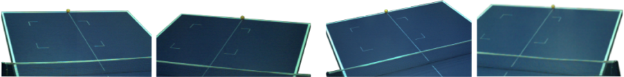
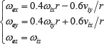
1. The aerodynamic model of the ping-pong ball

A standard ping-pong ball in the air is subjected to four forces: the gravity F _g , the air buoyancy force F _b , the air resistance F _d and the magnus force F _m .

${\displaystyle \sum }F=F_g+F_b+F_d+F_m$

(1)

Here, F _g =mg where m is the mass of the ball, g is the gravitational acceleration of the earth. F _b = -m_bg where m_b is the mass of the air that a ping-pong ball occupies. $F_d=-\frac{1}{2}{C}_D{\rho }_a\pi r^2\Vert v\Vert v$ where C_D is the drag coefficient of the ping-pong ball, ρ is the density of the air, r is the radius of the standard ping-pong ball, v is the linear velocity of the ping-pong ball. $F_m=-C_m{\rho }_a\pi r^3\omega \times v$ where C_m is the Magnus coefficient, ω is the angular velocity of the ping-pong ball. Equation (1) can be rewritten as:

${\displaystyle \sum }F=mg-m_{b}g-\frac{1}{2}{C}_D{\rho }_a\pi r^2\Vert v\Vert v-C_m{\rho }_a\pi r^3\omega \times v$

(2)

Since m_b< <m, we ignore the second item of Equation (2) and get

$\stackrel{.}{v}\left(t\right)=g-k_d\Vert v\Vert v+k_m\omega \times v$

(3)

or

$\begin{array}{ll}v(t_i)\hfill & =v\left(t_{i-1}\right)+\left[\begin{array}{ccc}-k_d\Vert v\Vert & -k_m{\omega }_z& k_m{\omega }_y\\ k_m{\omega }_z& -k_d\Vert v\Vert & -k_m{\omega }_x\\ -k_m{\omega }_y& k_m{\omega }_x& -k_d\Vert v\Vert \end{array}\right]\hfill \\ \hfill & \cdot v\left(t_{i-1}\right)\left(t_i-t_{i-1}\right)+\left[\begin{array}{c}0\\ 0\\ -g\end{array}\right]\left(t_i-t_{i-1}\right)\hfill \end{array}$

(4)

Where $k_d=C_D{\rho }_a\pi r^2/2m$ and $k_m=C_m{\rho }_a\pi r^3/m$ . The parameters ${\rho }_a=1.29kg/m^3,r=0.02m,m=0.0027kg,C_D=0.4997,C_m=1$ They are constants of a standard ping-pong ball k_d and k_m are therefore 0.15 and 0.012 respectively.

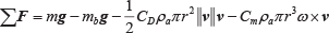
Since the linear velocity of a ping-pong ball is the derivative of its position, we can get:

$v\left(t\right)=\stackrel{.}{p}\left(t\right)$

(5)

or

$p\left(t_i\right)=p\left(t_{i-1}\right)+v\left(t_{i-1}\right)\left(t_i-t_{i-1}\right)$

(6)

Given the initial linear velocity v₀ ^b (Here, superscript b indicates the data belongs to trj-b, subscript 0 indicates the data is at the start time t₀ of trj-b), the initial angular velocity v₀ ^b and the initial ball position p₀ ^b at the start of trj-b (the same as the parameters at the end of trj-a), we can predict the trajectory of the ping-pong ball in trj-b by using equations (4) and (6) assuming that the angular velocity is constant in the air. Meanwhile, given the initial linear velocity v₀ ^d , the initial angular velocity ω₀ ^d and the initial ball position p₀ ^d at the start of trj-d (the same as the parameters at the end of trj-c), we can predict the trajectory of the ping-pong ball in trj-d in the same way.

Equations (4) and (6) form the aerodynamic model used to predict the following position and linear velocity of the ball. We will show the details of detecting and computing p₀^b, v₀ ^b , ω₀ ^b (also p₀ ^d , v₀ ^d , ω₀ ^d ) in section 4.2.

2. The rebound model of the ping-pong ball

In trj-c, the ping-pong ball hits the table and rebounds off. During this procedure, the linear velocity and angular velocity of the ball change immediately. The linear velocity and angular velocity may be decelerated or accelerated. Energy transforms from translation to rotation or vice versa.

We use a non-linear rebound model to predict the change of linear and angular velocities. Unlike the previous work [43, 42, 10] which assumes zero or constant horizontal restitution coefficients, we insist that the emergent velocity of a ping-pong ball is related to the friction coefficient. We can use impulse momentum theorem to build the rebound model. We assume that: (a) The emergent velocity along the z axis is proportional to the incident velocity along the z axis, namely v_ez=-k_vv_iz. Here, v_iz is the incident velocity along the z axis. v_ez is the emergent velocity along the z axis. k_v is named the vertical restitution coefficient. (b) The emergent spin around the z axis is equal to the incident spin around the z axis, namely ω _ez =ω _iz . Since the contact point between the ping-pong table and the ping-pong ball during rebound is on the spin axis or the z axis, the ping-pong table does not exert any torque around the z axis on the ball, and there is no reason to change the spin around the z axis. (c) The direction of the horizontal velocity of the ping-pong ball at the contact point does not change. It is either the same as the incident velocity or zero, namely $atan2\left(v_{bey}\mathrm{,}{v}_{bex}\right)=atan2\left(v_{biy}\mathrm{,}{v}_{bix}\right)$ or $v_{bex}=v_{bey}=0$ . Here, atan2() is an arctangent function with two arguments to return the appropriate quadrant as well as the angle. (v_bex, v_bix) and (v_bey, v_biy) are the emergent and incident velocities of the ping-pong ball at the contact point along the x and y axes, respectively.

Fig.4 illustrates the rebound procedure in a 3D view. Since the changes in v_z and ω _z have been analysed in assumptions (a) and (b), we do not need to consider the velocities related to the z axis. We can simplify our analysis by projecting the rebound into the xoz plane and the yoz plane (see Fig.5).

Figure 4.

3D view of the incident and the emergent linear velocities and angular velocities during the rebound procedure. The v_i, v_e, ω _i and ω _e are linear and angular velocities at the centre of the ping-pong ball (In contrast, the v_bi and v_be are linear velocities of of the ball at the contact point.

Figure 5.

2D view of the rebound procedure from the xoz plane (left) and the yoz plane (right)

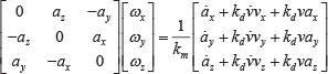
Take the xoz plane for example, from impulse momentum theory we can get

$\{\begin{array}{l}{v}_{bix}=v_{ix}-{\omega }_{iy}r\hfill \\ S_x=m\left(v_{ex}-v_{ix}\right)\hfill \\ S_{x}r=I\left({\omega }_{iy}-{\omega }_{ey}\right)\hfill \end{array}$

(7)

Here, v_bix is the incident velocity of the ping-pong ball at the contact point along the x axis. v_ix is the incident velocity at the centre of the ping-pong ball along the x axis. v_ex is the emergent velocity at the centre of the ping-pong ball along the x axis. ω_iy is the incident angular velocity around the y axis. ω_ey is the emergent angular velocity around the y axis. r is radius of a standard ping-pong ball. I=2mr²/3 is the inertia of a standard ping-pong ball. S_x is the impulse momentum exerted by the friction force along the x axis on the surface of the ping-pong table during rebound.

The friction force can be derived as follows. The impulse momentum of the friction force during rebound can be written as

$F_f\cdot \Delta t=\mu N\cdot \Delta t$

(8)

Here, F_f is the friction force, μ is the friction coefficient of the ping-pong table, N is the rebound force in the z axis and Δt is the duration of rebound. Since the product N · Δt is the impulse momentum along the z axis, it is equal to m(v_ez-v_iz). Therefore, Equation (8) can be rewritten as

$F_f\cdot \Delta t=\mu m\left(v_{ez}-v_{iz}\right)=\mu m\left(1+k_v\right)\left|v_{iz}\right|$

(9)

S_x can be computed by

$S_x=-F_f\cdot \Delta t\cdot \cos \theta =-\mu m\left(1+k_v\right)\left|v_{iz}\right|\cos \theta$

(10)

Here, θ is the angle between $\overrightarrow{\left\{v_{bix}\mathrm{,}{v}_{biy}\right\}}$ and the x axis. The minus symbo indicates that the direction of the friction is along $-\overrightarrow{\left\{v_{bix}\mathrm{,}{v}_{biy}\right\}}$ . Likewise, we can get

$\{\begin{array}{l}{v}_{biy}=v_{iy}+{\omega }_{ix}r\hfill \\ S_y=m\left(v_{ey}-v_{iy}\right)\hfill \\ S_{y}r=I\left({\omega }_{ex}-{\omega }_{ix}\right)\hfill \end{array}$

(11)

by analysing the xoy plane. Here, S_y can be computed by

$S_y=-\mu m\left(1+k_v\right)\left|v_{iz}\right|\sin \theta$

(12)

Note that we represent cosθ and sinθ with v_bix and v_biy, and get

$S_x=\frac{-\mu m\left(1+k_v\right)\left|v_{iz}\right|v_{bix}}{\sqrt{v_{bix}^2+v_{biy}^2}}$

(13)

$S_y=\frac{-\mu m\left(1+k_v\right)\left|v_{iz}\right|v_{biy}}{\sqrt{v_{bix}^2+v_{biy}^2}}$

(14)

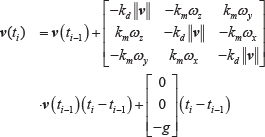
Substitute equations (7) and (11) with equations (13) and (14), we get

$\{\begin{array}{l}{v}_{ex}=\frac{\mu \left(1+k_v\right)\left|v_{iz}\right|\left({\omega }_{iy}r-v_{ix}\right)}{\sqrt{{\left(v_{ix}-{\omega }_{iy}r\right)}^2+{\left(v_{iy}+{\omega }_{ix}r\right)}^2}}+v_{ix}\hfill \\ v_{ey}=\frac{\mu \left(1+k_v\right)\left|v_{iz}\right|\left(-{\omega }_{ix}r-v_{iy}\right)}{\sqrt{{\left(v_{ix}-{\omega }_{iy}r\right)}^2+{\left(v_{iy}+{\omega }_{ix}r\right)}^2}}+v_{iy}\hfill \\ v_{ez}=-k_v{v}_{iz}\hfill \end{array}$

(15)

$\{\begin{array}{l}{\omega }_{ex}={\omega }_{ix}+\frac{3\mu \left(1+k_v\right)\left|v_{iz}\right|\left(-{\omega }_{ix}r-v_{iy}\right)}{2r\sqrt{{\left(v_{ix}-{\omega }_{iy}r\right)}^2+{\left(v_{iy}+{\omega }_{ix}r\right)}^2}}\hfill \\ {\omega }_{ey}={\omega }_{iy}-\frac{3\mu \left(1+k_v\right)\left|v_{iz}\right|\left({\omega }_{iy}r-v_{ix}\right)}{2r\sqrt{{\left(v_{ix}-{\omega }_{iy}r\right)}^2+{\left(v_{iy}+{\omega }_{ix}r\right)}^2}}\hfill \\ {\omega }_{ez}={\omega }_{iz}\hfill \end{array}$

(16)

Then, we can explicitly obtain the relationship between the emergent and incident velocities of the ping-pong ball at the contact point by

$\{\begin{array}{l}{v}_{bex}=v_{ex}-{\omega }_{ey}r=v_{bix}\left(1-\frac{2.5\mu \left(1+k_v\right)\left|v_{iz}\right|}{\sqrt{{\left(v_{ix}-{\omega }_{iy}r\right)}^2+{\left(v_{iy}+{\omega }_{ix}r\right)}^2}}\right)\\ v_{bey}=v_{ey}+{\omega }_{ex}r=v_{biy}\left(1-\frac{2.5\mu \left(1+k_v\right)\left|v_{iz}\right|}{\sqrt{{\left(v_{ix}-{\omega }_{iy}r\right)}^2+{\left(v_{iy}+{\omega }_{ix}r\right)}^2}}\right)\end{array}$

(17)

Note that the direction of the horizontal velocity of the ping-pong ball at the contact point does not change Therefore, $\left(1-\frac{2.5\mu \left(1+k_v\right)\left|v_{iz}\right|}{\sqrt{{\left(v_{ix}-{\omega }_{iy}r\right)}^2+{\left(v_{iy}+{\omega }_{ix}r\right)}^2}}\right)$ should be larger than or equal to zero, namely

$\frac{\mu \left(1+k_v\right)\left|v_{iz}\right|}{\sqrt{{\left(v_{ix}-{\omega }_{iy}r\right)}^2+{\left(v_{iy}+{\omega }_{ix}r\right)}^2}}\le 0.4$

(18)

If $\frac{\mu \left(1+k_v\right)\left|v_{iz}\right|}{\sqrt{{\left(v_{ix}-{\omega }_{iy}r\right)}^2+{\left(v_{iy}+{\omega }_{ix}r\right)}^2}}$ is smaller than 0.4, we directly use equations (15) and (16) to compute the linear velocity and angular velocity after rebound.

If $\frac{\mu \left(1+k_v\right)\left|v_{iz}\right|}{\sqrt{{\left(v_{ix}-{\omega }_{iy}r\right)}^2+{\left(v_{iy}+{\omega }_{ix}r\right)}^2}}$ is equal to 0.4, equations (15) and (16) become

$\{\begin{array}{l}{v}_{ex}=0.4{\omega }_{iy}r+0.6v_{ix}\hfill \\ v_{ey}=-0.4{\omega }_{ix}r+0.6v_{iy}\hfill \\ v_{ez}=-k_v{v}_{iz}\hfill \end{array}$

(19)

$\{\begin{array}{l}{\omega }_{ex}=0.4{\omega }_{ix}r-0.6v_{iy}/r\hfill \\ {\omega }_{ey}=0.4{\omega }_{iy}r+0.6v_{ix}/r\hfill \\ {\omega }_{ez}={\omega }_{iz}\hfill \end{array}$

(20)

We use them to compute the linear velocity and angular velocity after rebound.

If $\frac{\mu \left(1+k_v\right)\left|v_{iz}\right|}{\sqrt{{\left(v_{ix}-{\omega }_{iy}r\right)}^2+{\left(v_{iy}+{\omega }_{ix}r\right)}^2}}$ is larger than 0.4, the direction of the horizontal velocity changes after rebound. This conflicts with our assumption (c) of the non-linear rebound model. In the worst case, the velocity of the ping-pong ball at the contact point should be 0. Therefore, we use the same equations under the condition that $\frac{\mu \left(1+k_v\right)\left|v_{iz}\right|}{\sqrt{{\left(v_{ix}-{\omega }_{iy}r\right)}^2+{\left(v_{iy}+{\omega }_{ix}r\right)}^2}}=0.4$ . That is, if $\frac{\mu \left(1+k_v\right)\left|v_{iz}\right|}{\sqrt{{\left(v_{ix}-{\omega }_{iy}r\right)}^2+{\left(v_{iy}+{\omega }_{ix}r\right)}^2}}$ is larger than 0.4, we still use equations (19) and (20) to compute the linear velocity and angular velocity after rebound.

Equations (15), (16), (19) and (20) form our non-linear rebound model. The output of this model will be used as the v₀ ^d and ω₀ ^d of trj-d to predict the trajectory in trj-d with the aerodynamic model.

4.2 Predicting trajectories with the physical models

Ball detection is the basis for trajectory prediction. In 4.2, we discuss the details of how to detect the positions of the ball in trj-a, how to estimate the initial linear and angular velocities of the ball at the start of trj-b, how to predict the trajectory of the ball in trj-b and trj-d with the aerodynamic model and how to predict the motion of the ball in trj-c with the non-linear rebound model.

1. Ball detection and parameter estimation to predict trj-b

Predicting the trajectory of the ball in trj-b with the aerodynamic model requires precisely and efficiently finding the initial trajectory parameters v₀^b, ω₀ ^b and p ₀ ^b from the detected positions of the ping-pong ball in trj-a.

We use thresholding plus elliptic fitting to detect the 2D position of the ball in each image from the working camera pair, and reconstruct the 3D position of the ball with stereo triangulation.

The thresholding involves an off-line training stage and an on-line filtering stage. During the off-line training stage, we collect many sample images containing one or more ping-pong balls at different locations in the view of the cameras. We compute the mean hue value and saturation value of each ping-pong ball in the sample images and get a colour range $h\in \left[H_{lo}\mathrm{,}{H}_{hi}\right]\mathrm{,}s\in \left[S_{lo}\mathrm{,}{S}_{hi}\right]$ as the thresholding model of a ping-pong ball. In the on-line filtering stage, we use this thresholding model to decide whether a pixel in a captured image belongs to the ping-pong ball. We group the likely pixels into candidate regions.

After that, we analyse the features of the candidate regions to get the best one. On the candidate regions obtained by thresholding, we apply regional operations such as closing, opening, filling and connection to the image regions to get larger region blocks. If a region has an area and circularity within a proper threshold, we take the region as the best candidate of a ping-pong ball.

Finally, we use elliptic fitting to detect the precise location of the ping-pong ball. The elliptic fitting involves a pre-processing stage and a fitting stage. In the pre-processing stage, we dilate the candidate region to enclose the contours of the ping-pong ball and use a Canny detector to extract these contours precisely. In the fitting stage, we unite the contours and fit them with an ellipse. The centre of the ellipse is the 2D position of the ping-pong ball.

Given detected 2D coordinates of a ping-pong ball in an image pair, we can use triangulation to reconstruct its 3D position. This is done by solving the linear equation

$\{\begin{array}{l}{x}_l=P_{l}p\hfill \\ x_r=P_{r}p\hfill \end{array}$

(21)

Where x_i and x_r are the 2D coordinates after distortion correction in the left camera and the right camera of a stereo pair. P_l and P_r are projection matrices of the left camera and right camera respectively. p is the 3D position of the ping-pong ball.

We reconstruct the positions of the ping-pong ball by using all the image pairs captured in trj-a and get the trajectory data ${\left\{p_i^a\mathrm{,}{t}_i\right\}}_{i=1\dots m_a}$ Here, superscript a indicates the data belong to trj-a. m_a denotes the number of image pairs captured in trj-a. t_i is the time of each reconstructed 3D position p _i ^a .

We smooth the trajectory data of trj-a by fitting them to a four-order polynomial

$f\left(t\right)={\displaystyle \sum _{k=0}^4}{\alpha }_k{t}^k$

(22)

and replacing p _i ^a with f(t_i). The smoothing process further reduces the noises of each individual p _i ^a. Note that we use a four-degree polynomial since it satisfies the continuity of the jerk and gives smooth accelerations on the trajectory.

Once we have replaced p _i ^a with f (t_i), we can compute the initial position p ₀ ^b = f (t_m) and the initial linear velocity $v_0^b=\stackrel{.}{f}\left(t_{m_a}\right)$ of trj-b.

Besides p^b₀ and v₀ ^b , we compute ω₀ ^b using

$\left[\begin{array}{ccc}0& a_z& -a_y\\ -a_z& 0& a_x\\ a_y& -a_x& 0\end{array}\right]\left[\begin{array}{c}{\omega }_x\\ {\omega }_y\\ {\omega }_z\end{array}\right]=\frac{1}{k_m}\left[\begin{array}{c}{\stackrel{.}{a}}_x+k_d\stackrel{.}{v}{v}_x+k_{d}v{a}_x\\ {\stackrel{.}{a}}_y+k_d\stackrel{.}{v}{v}_y+k_{d}v{a}_y\\ {\stackrel{.}{a}}_z+k_d\stackrel{.}{v}{v}_z+k_{d}v{a}_z\end{array}\right]$

(23)

This equation is obtained by differentiating Equation (3). We can get the initial angular velocity ${\omega }_0^b={\left[{\omega }_0^b{}_x\mathrm{,}{\omega }_0^b{}_y\mathrm{,}{\omega }_0^b{}_z\right]}^T$ by replacing the ${\left[v_x\mathrm{,}{v}_y\mathrm{,}{v}_z\right]}^T,{\left[a_x\mathrm{,}{a}_y\mathrm{,}{a}_z\right]}^T$ , and ${\left[{\stackrel{.}{a}}_x\mathrm{,}{\stackrel{.}{a}}_y\mathrm{,}{\stackrel{.}{a}}_z\right]}^T$ in this equation with v₀ ^b , $a_0^b={\stackrel{.}{v}}_0^b$ , and ${\stackrel{.}{a}}_0^b={\stackrel{..}{v}}_0^b$ . Note that we assume the angular velocity of the ball does not change during flying: ω _i ^b = ω₀ ^b .

With p₀ ^b , v₀b and ω _i ^b, we can predict the trajectory data ${\left\{p_i^b\mathrm{,}{v}_i^b\mathrm{,}{t}_i\right\}}_{i=1\dots m_b}$ of the ping-pong ball in trj-b by iteratively using equations (4) and (6). Like ${\left\{p_i^a\mathrm{,}{t}_i\right\}}_{i=1\dots m_a}$ , the superscript b indicates the data belong to trj-b. m_b denotes the number of points predicted in trj-b. Note that since $p_i^b={\left[p_i^b{}_x\mathrm{,}{p}_i^b{}_y\mathrm{,}{p}_i^b{}_z\right]}^T,v_i^b={\left[v_i^b{}_x\mathrm{,}{v}_i^b{}_y\mathrm{,}{v}_i^b{}_z\right]}^T$ and the iteration stops when p^b_iz=r, the total number of points m_b is obtained at the point where p^b_mbz = r.

2. Predicting the change of the ball's motion in trj-c and the trajectory of the ball in trj-d

The velocities v^b_mb and ω ^b _mb of the ball at the last point p_mb^b of the predicted trj-b will be used as the incident linear velocity v_i =[v_ix,v_iy,v_iz] ^T and the incident angular velocity ω _i =[ω _ix , ω _iy , ω _iz ] ^T of the rebound model to predict the change of the ball's motion in trj-c according to equations (15) and (16) when Equation (18) is satisfied or equations (19) and (20) when Equation (18) is not satisfied.

The output of the rebound model will be the emergent linear velocity v_e=[v_ex,v_ey,v_ez] ^T and the emergent angular velocity ω _e =[ω _ex , ω _ey , ω _ez ] ^T . The initial linear velocity of trj-d is v₀ ^d =v _e , The initial position of trj-d is the same as p₀ ^d = p_m^b_b, and the angular velocity ω _i ^d is also assumed to be constant, the same as ω₀ ^d = ω _e in trj-d. We use v₀ ^d , p₀ ^d and ω _i ^d to predict the trajectory data {p_i^d,v_i^d,t_i} _i =1… _md in trj-d.

Note that we set the opponent robot to return the ball at a fixed vertical plane x = p_x which is called the ball returning plane ¹ . Therefore, the total number of points m_d in trj-d is obtained at the point where $p_{m_b}^b{}_z=r$ . We send the p_m^d_d, t_m^d_d, v_m^d_d and ω _m ^d _d to the robot controllers to plan motions for ball returning.

Fig.6 summarizes the flow of predicting trj-b, trj-c and trj-d with the aerodynamic model and the non-linear rebound model. We will analyse their performance in Section 5.

Figure 6.

The flow of predicting trj-b (orange box), trj-c (red box), and trj-d (blue box) with the aerodynamic model (trj-b and trj-d) and the non-linear rebound model (trj-c)

5. Experiments and Analysis

We carry out three groups of experiments to verify the performance of our vision module. In the first group, we analyse the precision and efficiency of the ball detection method through comparison of the perceived positions with manually measured positions of randomly placed ping-pong balls at different x,y,z positions in the view of the cameras. In the second group, we present the results of our prediction method and compare these results with an LWR-based prediction method to show our advantages. In the third group, we integrate the vision module into a real game and demonstrate its performance in a ping-pong game played by two BHR-5 humanoid robots.

5.1 Perception precision and efficiency

We first present a sample trajectory as well as the predicted result. Then we will analyse the perception precision and efficiency in detail.

1. A sample trajectory and the predicted hitting point

We would like to show an exact measured three dimensional ping-pong trajectory and the actual prediction result point obtained by our vision module in Fig.7. The dashed points are the measured 3D trajectory, and the star point is the predicted hitting point. We can see that the predicted point is rather close to the perceived trajectory. The perception precision and efficiency will be analysed in the remainder of this subsection. The prediction precision will be evaluated in the second group of experiments presented in the next subsection by comparing the predicted results with the perceived trajectories.

Figure 7.

A sample trajectory and the predicted result. The dashed points are trajectory points and the star is the predicted hitting point.

2. Inherent perception errors

Due to the resolution of digital cameras, there are some inherent perception errors for ball detection. Theoretically, the inherent perception error of a stereo camera pair in each axis has the form of

$\Delta x=\frac{z\Delta u}{f}\mathrm{,}\Delta y=\frac{z\Delta u}{f}\mathrm{,}\Delta z=\frac{z^2\Delta u}{fb}$

(24)

Where Δu is the image detection error, f is the focus of the cameras, and b is the length of the baseline.

For the cameras used in our vision module, f = 12mm, b=2.32m, the pixel size is 7.4um, and the furthest depth of view is around 4.45m. Suppose the ball detection error is 1 pixel, then Δu=7.4um. The maximum inherent perception errors are $\Delta x=\Delta y=4.45\times 7.4\times {10}^{-6}/\left(12\times {10}^{-3}\right)=2.7mm$ and $\Delta z={4.45}^2\times 7.4\times {10}^{-6}/\left(12\times {10}^{-3}\times 2.32\right)=5.26mm$ .

The perception error is inherent to the image detection error Δu. If we want to reduce the reconstruction error of the vision module, the key is to reduce the image detection error Δu.

3. Detection and reconstruction error

We would like to analyse the detection and reconstruction error of the vision module by randomly placing the ping-pong ball at 22 different x,y,z positions in the view of the cameras. We measure each position 800 times using the vision module and compare them with the ground truth value. The errors (standard deviations with respect to their real-world coordinates) along the x, y and z axes are shown in Fig.8. They are less than 10mm (less than 4mm on average).

Figure 8.

The measuring errors (standard deviations with respect to their real-world coordinates) along x, y, and z axes

4. Efficiency

The sampling rate of our cameras before applying detection and reconstruction algorithms is 202 fps. We also use the MVTec's HALCON machine vision tool to speed up the detection and reconstruction process. However, the perception speed will still be reduced due to the time used for detection, construction and prediction. We have performed three experiments to measure the perception speed as well as prediction time.

The first experiment is the time interval of the exact sample trajectory (Fig.7) WITH prediction (prediction will only be executed at the end of perception of trj-a). The absolute time of each trajectory is recorded according to CPU time, which means that the time includes all operations including, but not limited to, image grabbing, detection, reconstruction and prediction. We have calculated the time intervals of each trajectory point with respect to the previous trajectory point of that trajectory. The time intervals are shown in Fig. 9. From the figure we can see that most of the time intervals are close to 8 ms. Therefore, the perception frequency is close to 1 s/8ms=120fps. Due to the prediction algorithm execution around absolute time 70.38 s, the detection and reconstruction process was delayed.

Figure 9.

The time interval of the sample trajectory for each frame

The second experiment is the perception frequency measurement experiment WITHOUT prediction. The frequency is calculated trajectory by trajectory. Table 1 shows the frame rate of 24 different sequences after applying grabbing, detection and reconstruction algorithms. The average frame rate of our vision module after applying grabbing, detection and construction is 121.9 fps.

Table 1.

Efficiency after applying grabbing, detection and reconstruction algorithms

index	speed(fps)	index	speed(fps)	index	speed(fps)
1	121.705481	9	121.858768	17	121.819488
2	122.024017	10	121.941730	18	121.939284
3	121.927763	11	121.830476	19	121.831608
4	121.946217	12	121.938105	20	121.957102
5	122.043332	13	122.014771	21	121.866378
6	121.904633	14	122.023197	22	121.999261
7	121.826457	15	122.098293	23	121.890278
8	121.848082	16	121.899356	24	122.031109

The third experiment is the prediction time measurement experiment. A trajectory may execute the prediction algorithm one time. We have measured the prediction time trajectory by trajectory. Table 2 shows the prediction time consumed by 24 different sequences. The average prediction time of our vision module is 12.049ms.

Table 2.

Prediction time for 24 trajectories

index	time(ms)	index	time(ms)	index	time(ms)
1	11.656	9	11.494	17	12.665
2	11.613	10	12.838	18	12.675
3	11.648	11	12.885	19	12.648
4	11.707	12	11.496	20	11.447
5	11.505	13	12.749	21	11.558
6	12.830	14	12.657	22	11.485
7	11.641	15	11.550	23	11.500
8	12.881	16	11.464	24	12.584

Therefore, our vision module has an average perception speed of 121.9 fps and a prediction time of 12.049ms for each trajectory. Comparing with the state-of-the-art vision modules designed for a robotic ping-pong game [23, 22, 15], the processing speed of our vision module with image size 640times480times3ch of four cameras at 120 fps over the standard sized ping-pong table is the second fastest.

5.2 Performance of prediction

In order to analyse the performance of our prediction method, we use 40 perceived trajectories of the ping-pong ball as the ground truth value. Then, for each of the 40 ground truth trajectories, we divide it into trj-a, trj-b, trj-c and trj-d, and use trj-a to predict trj-b, trj-c and trj-d following the flow in Fig.6. By comparing the predicted trajectories trj-b, trj-c and trj-d with the ground truth value or the detected trajectories, we can easily see the precision of our prediction method. Moreover, we implement the conventional LWR-based prediction method and compare the results of LWR based prediction method on the 40 trajectories with ours.

Fig.10 shows one case of the 40 results. Both our prediction method and the LWR-based prediction method are able to predict the remaining trajectories. Nevertheless, our prediction method is better in fitting the trajectories, especially in fitting the trajectories after rebound. The nonlinear rebound model used in our prediction method better describes the energy transform between translation and rotation (compare the green and yellow points in Fig.10).

Figure 10.

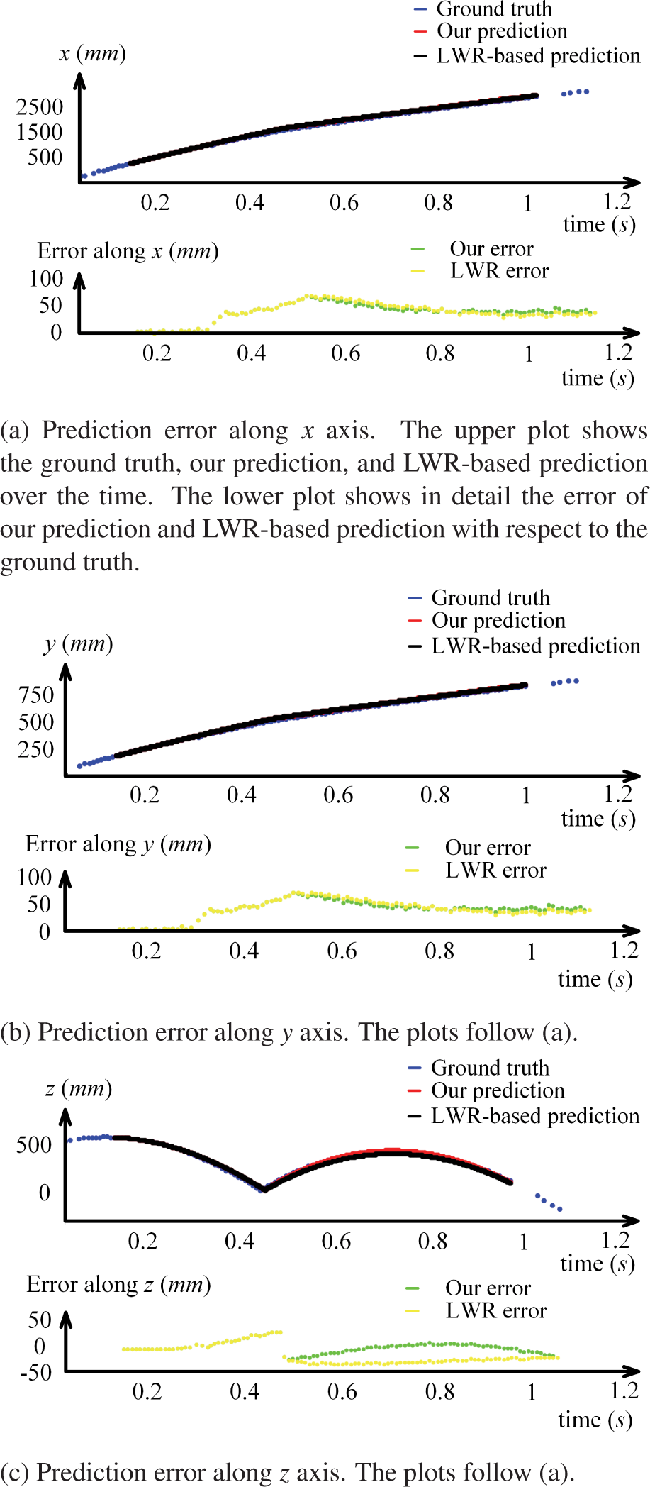
One case of the 40 results

Fig.12 shows the average prediction error of our prediction method and the LWR-based prediction method with respect to the ground truth value of the 40 trajectories. The mean average prediction error of each trajectory along the y axis is less than 30mm and the average prediction error of each trajectory along the x and z axes is less than 50mm for both methods. In all, our prediction method outperforms the LWR-based prediction method: Most of the error of our prediction method along the z axis is smaller than 20mm. In contrast, the error of the LWR-based prediction method is larger than 30mm. There is a significant improvement of our approach on predicting the trajectories in the z axis. The error of our prediction method along x axis and y axis is also smaller than the LWR-based prediction method. Our trajectory prediction method is more precise than LWR-based approach.

Figure 11.

A sequence of snapshots during the robot-robot ping-pong game. Images 1 and 2 belong to trj-a. Image 3 belongs to trj-b. Image 4 belongs to trj-c. Images 5 and 6 belong to trj-d. Images 7, 8, and 9 belong the trajectories in a second round.

Figure 12.

Average prediction errors of our prediction and the LWR based prediction with respect to the ground truth values. Red curve: Our prediction; Blue curve: LWR based prediction. Vertical axis: The error (difference from ground truth value) of prediction; Horizontal axis: The index of the 40 trajectories.

At the ball returning plane x= p_xr, as is shown in Fig.13, the average prediction error of the 40 trajectories along x, y, and z axes is less than 50mm. This is small enough for a standard ping-pong racket (158mmx152mm).

Figure 13.

The average prediction errors of the 40 trajectories along x, y, and z axis at the receiving and returning plane x=p_xr

5.3 Integration into a real humanoid robotic ping-pong game

We integrate the vision module into a real humanoid robotic ping-pong game and use the predicted results to actuate two BHR-5 humanoid robots to play with each other. The vision module enables the two robots to continuously play ping-pong for more than 200 rounds. Fig.11 shows a sequence of snapshots during the game. Moreover, the vision module can also be integrated into a human-robot ping-pong game. Interested readers may go to http://goo.gl/LJfKcE to see the full video clips of the robot-robot game and the human-robot game.

6. Conclusion

In this paper, we presented a precise yet efficient vision module for a humanoid robotic ping-pong game. The vision module has two pairs of 640times480times3ch cameras with each pair perceiving one half of the ping-pong table. It uses thresholding and elliptic fitting to detect the 2D positions, stereo triangulation to reconstruct the 3D positions, an aerodynamic model to predict the trajectories of the ball in the air and a novel non-linear rebound model based on impulse momentum theorem to predict the change of the ball's motion during rebound. The vision module has a prediction error less than 50 mm and a processing speed of 120fps. With this vision module, two humanoid robots can play ping-pong with each other continuously for more than 200 rounds.

Through various experiments and analysis, we conclude that: (1) The approach of using two stereo camera pairs to perceive the ping-pong table and using thresholding and elliptic fitting to detect 2D positions is precise and efficient for trajectory perception. (2) The approach of using the perceived trajectory trj-a plus the aerodynamic model and the novel non-linear rebound model to predict the trajectories trj-b, trj-c and trj-d is precise for trajectory prediction and spares enough time for humanoid ping-pong players' responses. The predictive vision module is proved to be robust in both the robot-robot and human-robot ping-pong game.