
Abstract
Pose estimation methods in robotics applications frequently suffer from inaccuracy due to a lack of correspondence and real-time constraints, and instability from a wide range of viewpoints, etc. In this paper, we present a novel approach for estimating the poses of all the cameras in a multi-camera system in which each camera is placed rigidly using only a few coplanar points simultaneously. Instead of solving the orientation and translation for the multi-camera system from the overlapping point correspondences among all the cameras directly, we employ homography, which can map image points with 3D coplanar-referenced points. In our method, we first establish the corresponding relations between each camera by their Euclidean geometries and optimize the homographies of the cameras; then, we solve the orientation and translation for the optimal homographies. The results from simulations and real case experiments show that our approach is accurate and robust for implementation in robotics applications. Finally, a practical implementation in a ping-pong robot is described in order to confirm the validity of our approach.
1. Introduction
Pose estimation from a referenced rigid structure is one of the most basic and important problems in robotics vision and computer graphics. It can be used to obtain the 6DOF (degrees of freedom) of the cameras needed for further implementation, e.g., in helping robots to locate targets in referenced coordinates [1, 2], in calculating coordinates in images of virtual 3D objects to synthesize augmented reality scenes [3], in locating flying balls for robots [4], and in calibrating the camera-laser sensor system [5].
Although the single camera pose estimation problem has been widely researched in the last decade, the methods used often suffer from low robustness and ill-conditioned pose estimation problems. Furthermore, a relatively small angle for viewing influences the accuracy of the estimated pose.
In practical robotics vision applications (e.g., catching objects via robot arms, playing ping-pong with robots, etc., all of which may require the vision system to perform in real-time), the tasks of pose estimation (which aim to locate the absolute coordinates of objects via the vision system of the robot) require quite a high degree of accuracy and robust performance in most conditions. A single camera cannot provide enough precision or robustness in such tasks for pose estimation, and thus a multiple camera system is required. Furthermore, task-related robots are normally required to obtain the absolute coordinates of a tracing target in the referenced space via rigid point correspondences from landmarks, while a single-camera system will obtain infinite solutions for the target due to the property of perspective projection.
In the specific case of mobile robots, pose estimation methods for multiple camera systems have always faced the following challenges:
In applications of mobile robots - especially in the case of robots working at high speed - to achieve the poses of all the cameras simultaneously is the most important requirement. Otherwise, the poses estimated individually will break the rigid constraint among all the cameras in the multiple camera system, as there may be some motion in the pose estimation of different cameras due to the high speed of the robot.
Methods are always required that can work accurately, stably (with low standard deviation - STD) and robustly under any angle of viewpoint due to the uncertain poses of mobile robots.
The task of localization is always followed by the task of pose estimation; thus, the methods should also provide preferable localization performance for their estimations.
As the movement of the robot may shake the rigid rig among the cameras and introduce bias, the pose estimation methods should also be robust in relation to the interference of bias on solid rigs.
Mobile robots are real-time systems, and so they require the pose estimation methods to calculate as quickly as possible and with fewer point correspondences, due to the mobility of a given view.
In this paper, we address all the above challenges and present a novel approach for estimating the poses of all the cameras in a multi-camera system with only a few coplanar points in a manner that is accurate, robust and simultaneous 1 , and we aim to resolve the above four main challenges as they arise in the practical vision system of a humanoid ping-pong robot.
2. Related Works
Pose estimation for single cameras [6–11] has been studied for many years. Recently, much of the research has focused on pose estimation in multi-camera systems, due to the limitations of single cameras, e.g., their low accuracy and limited field-of-view.
One of the most important advantages of a multi-camera system is that it can recover stereo information easily (e.g., the visual odometry [12], which employs calibrated cameras to recover the 3D information of targets), and it can help to estimate the motion of the cameras from the optical flow via the Kalman filter method or by minimizing a cost function based on the geometric and 3D properties of the features.
Generally, there are two kinds of multi-camera systems: one is designed for overlapping fields of view [13–17] and the other for non-overlapping fields of view [18, 19].
The methods for a non-overlapping system [18, 19] require the use of cameras which are placed rigidly on a moving object, where the translation and rotation between the cameras are known. When the object is moving rigidly, these methods can recover the 6DOF motion for the multi-camera system via the point correspondences between two points seen before and after motion. These methods are normally implemented on a vehicle or other moving objects, and require relative motion between every other image.
The methods for overlapping systems also employ cameras placed rigidly, with known translation and rotation between each camera, and they can recover the pose of their systems with only one frame of the multiple images from different cameras. As such, these methods can be used to process static scenes. As there are many efficient pose estimation methods for single cameras, an intuitive solution for overlapping fields of view in multi-camera systems is to estimate the pose for each camera and then reduce the ambiguities produced by the estimated poses of every camera based on their rigid constraint via fusing or polling policies. The methods presented by Baker et al. [14] and Viksté et al. [15] belong to this category. However, this kind of method does not obtain a unifying pose for the multi-camera system with all the information from all the cameras simultaneously. It may introduce some inconsistencies with the rigid constraint between each pair of cameras, which may reduce the precision of multi-camera systems for measurement or object localization (i.e., stereo vision for grasping with robots [20]). In this paper, we present a novel approach which estimates the pose of a multi-camera system with overlapping fields of view and can calculate the unifying pose for the system with all the information from all the cameras simultaneously.
3. Our Approach to Pose Estimation for Multi-camera Systems
Pose estimation for a multi-camera system should calculate the orientation and translation with the rigid pose constraint among the various cameras. Most existing methods attempt to solve the orientation and translation directly, by optimization [21] or iteration [11, 22]. In contrast, we employ homography, which is widely implemented in calibration [23, 24] and can map image points with 3D coplanar referenced points. Firstly, we establish the corresponding relations between each camera using their Euclidean geometries and optimize the homographies of the cameras; then, we solve the orientation and translation from the optimal homographies.
3.1 Problem definitions
The intrinsic parameters of the ith camera in a multi-camera system are denoted by

The task of estimating the absolute pose of a multi-camera system can be formalized as follows. Given a set of coplanar non-collinear 3D coordinates of referenced points
3.2 Homography for coplanar corresponding points
The homogeneous coordinate of the referenced point

Here, s is an arbitrary scale factor,

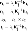
λ
j
= 1/ ‖
3.3 The global optimum for multi-camera systems
In our approach, we try to minimize the image distances of all the cameras with respect to the referenced coplanar points.
Given n referenced coplanar points and k cameras, we can estimate the homography (
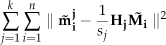
The above optimal function is established on the assumption that the image points of each camera are perturbed by Gaussian noise, which is quite usual in many image noise removal methods [25–27] and vision practices [28–30]. For cameras that are assembled rigidly, the homography of each camera has inherent constraint relations, which will help us to obtain the global optimization for the multi-camera system using only a few points.
3.4 Extrinsic translation for multiple cameras with homography
In this section, we will present the method for the calculation a camera's homography from one known homography with known rigid rotation and translation. Assume that there are two cameras, i and j, with a rigid rotation matrix
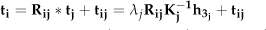

Thus, the homography of camera i has the following relation based on the definition of homography in equation (3):

The above formulation presents only the scale transformation relation between the homographies of two different cameras. However, in our approach, the homography is defined with the scale H(3,3) = 1, and so the homography of

With homography
Accordingly, the optimization function in (5) can be rewritten as:

Here, the scale factor sj can be calculated with the following formula:

3.5 Estimation of the initial homography
The solution for the formula (10) is a typical nonlinear optimization problem. In our approach, the Levenberg-Marquardt method is adopted, which has been widely used in computer vision cases. When solving the optimization with formula (10), an initial guess for
The method to calculate the initial homography

Since
Before calculating the initial guess as to the homography using the above method, the data should first be normalized [28] to obtain more stable and accurate results.
If a more accurate initial guess for the homography is desired, the maximum likelihood estimation of
Such that
The optimization of the above function can also be solved using the Levenberg-Marquardt method, and the initial guess can be obtained with the solution to equation (12).
4. Experiments
We compared our method with various state-of-the-art methods, using both simulations and real image data. Finally, we present the practical implementation of our method in ping-pong robots.
In the following experiments, we used seven pose estimation methods.
MAAMC, the method introduced in this paper (abbreviated as MAAMC) to obtain the pose of the multi-camera system simultaneously.
SAAMC, a simplified version of our MAAMC - it separates the computation of the homography for each camera and then obtains the pose of each camera individually with formula (3).
LHM, the method presented by Lu et al.. [11], which is an efficient iterative approach for estimating the pose for a single camera. This method has been shown to be capable of dealing with arbitrary numbers of correspondences and achieves excellent precision when it converges properly 3 . We used LHM to estimate the pose of each camera individually.
MLHM [17], an enhancement of LHM, which transfers all the cameras into one unified coordinate and minimizes the total errors in 3D referenced space iteratively. This method can also obtain the 6DOF pose of the multi-camera system simultaneously. In our experiments, weak-perspective models were used to obtain the initial estimations for both LHM and MLHM.
JKR [16], a method which can estimate the poses of each camera simultaneously.
RPP [10], a robust pose estimation method from a planar target presented by Schweighofer. It estimates each camera's pose individually.
MAACM - MLHM, a hybrid method which employs our initial pose estimation method to obtain the initial estimation for MLHM.
The above seven methods could be classified according to three categories. One set includes the methods 4 estimated from coplanar points, e.g., MAAMC, SAAMC and RPP. The second set includes the methods 5 estimated from non-coplanar points, e.g., LHM and MLHM. The last method is MAACM − MLHM 6 , which is a premium version of MLHM with an initial R estimated by MAACM.
With the above seven methods, MLHM,MAAMC,JKR and MAAMC − MLHM were all able to obtain the poses of each camera simultaneously, while the other approaches needed to estimate the pose of each camera one by one.
4.1 Simulation experiments
In these experiments, we simulated several cameras placed rigidly. The distances 7 between cameras were about 100. Each camera's focal length ratio was set as fu = fv = 540 and the simulation resolution was 640×480; thus, the principal point was located at the pixel point (U0, V0)=(320,240). The Gaussian noise for the corresponding 2D point coordinates was also included in the simulation model.
We used the relative error to evaluate the experimental results. Given the true results of camera i,


where n is the total number of cameras in the system, and
To evaluate the effect of the estimation when the two cameras are placed and subject to different amounts of rigid motion, all the simulation experiments were designed with random relative positions of the camera, which was achieved by limiting three axis-rotation angles with intervals of [0,2] degrees, translation vectors from [50,0,0] to [60,10,10], and while controlling all the reference points in the overlapping view.
4.1.1. Simulation experiments for R, T, localization and re-projection error
As the performance of the pose estimation methods may be influenced by the viewing angle, we evaluated the performance (R, T, localization and image re-projection error) of the above methods given small viewing angles (which occurred quite frequently in the humanoid ping-pong robot).
In the simulation experiment, the 3D referenced points were restricted in the plane with z = 0, x ε [−200,200] and y ε [−300,300]. The cameras were placed within the conic area (the vertex was (0,0,0)), where the distribution intervals were z ε [1500,1700], x ε [−980,980] and y ε [2500,3200]. The experimental results are shown in figure 1 and figure 2.
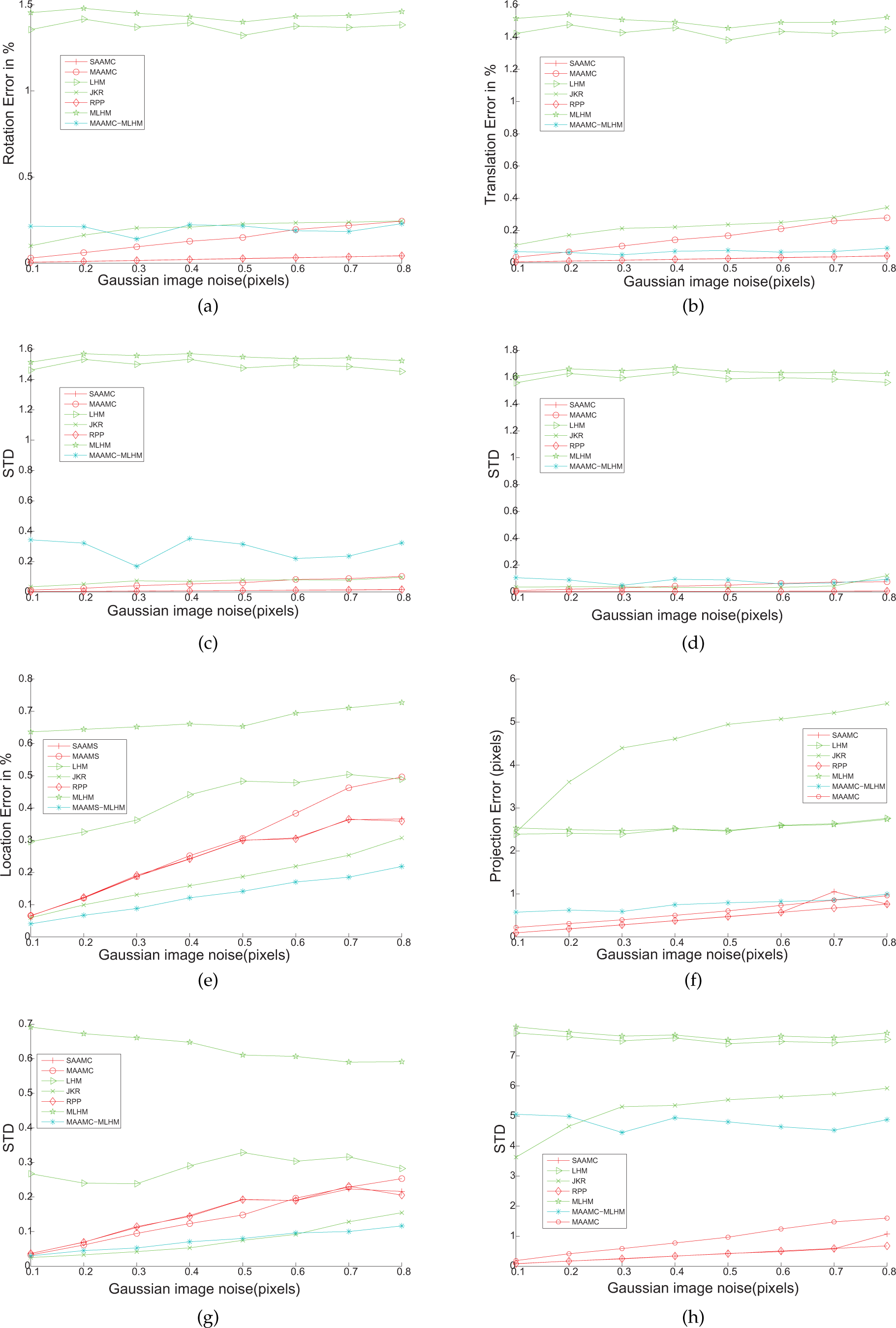
Simulation experiment results under varied Gaussian noise. There were two cameras in the multi-camera system using eight referenced points. (c),(d),(g) and (h) are the corresponding standard deviations of (a),(b),(e) and (f).

Simulation experiment results under varied referenced points. There were two cameras in the multi-camera system using Gaussian noise σ = 0.5. (c),(d),(g) and (h) are the corresponding standard deviations of (a),(b),(e) and (f).
We also carried out an experiment to evaluate the absolute locating performances of these methods 8 . When executing the pose estimation, a noised point (with a ground true value P(430, 760, 200)) was generated out of the plane of referenced points, and we used the estimated pose of each camera to estimate the coordinate of point P with its image (with the same Gauss noise as the referenced points) in each camera. Its position in the referenced coordinates was calculated by taking a radial from the centre of the projection of each camera to the image of P in that camera, and calculating the middle points of the perpendicular bisectors between every two radials. The estimated P˜ was then obtained by averaging all the middle points. The experimental results from the locating method are shown in figure 1 and figure 2 (e) and (g).
According to figure 1(a),(b),(c) and (d), we can see that the object space-minimizing-based approaches, i.e., MLHM and LHM, will be much worse than the other approaches for small angle of viewing conditions with increasing noise. The reason may be that the initial guesses of MLHM and LHM are normally far from the true pose when the viewing angles are small; thus, they will converge on another local minimum. That is why MAACM − MLHM will achieve a better performance with a better initial guess from MAACM. With such small angle viewing conditions, RPP has a special optimization to avoid converging on the local minimum so that it can achieve the same best performance as our SAACM approach for pose estimation.
According to figure 2(a)–(d), we can see that the object space-minimizing-based approaches, i.e., MLHM, LHM will be quite unstable for pose estimation for small viewing angles. Figure 2(e) and (g) also show that the approaches estimating poses simultaneously will achieve better performances than those doing so individually for localization.
The simulation experimental results also show that the pose estimation for each camera in turn could perform as well as the global optimization methods; however, the performances in localization with those methods estimated one by one were always worse than the global methods. In our view, the reason for this may be that the global optimization methods always consider the rigid rig as the constraint in optimization, which may lead to greater compromise in the computation of the average system bias. However, the method optimizing singly can ignore this constraint and converge on those poses with less system bias, while the real rig is broken and leads to poor performance in localization applications.
4.1.2. Simulation Experiments on Other Metrics
In the second simulation experiment, we further evaluated four approaches, i.e., JKR, MLHM, MAAMC and MAAMC − MLHM, all which estimated the poses of all the cameras simultaneously.
We first evaluated the performances of the four approaches for different mounted cameras. Figure 3 shows the experimental results after using various numbers of cameras (3–5) in the multi-camera system. In this experiment, we randomly chose 25 poses for the multi-camera system, which were distributed in the half sphere towards the original centre (0,0,0) with a distance of 1,500, and then executed the estimation 200 times to output the average. The results in figure 3 show that the performances of all four methods will increase as the number of cameras increases. Although the number of cameras has been increased, the MLHM will also be suffered with wrong initial values - this is why the MLHM performances were worst while the MAACM − MLHM performances were almost the best with a good initial value from our MAACM.

Simulation experiment results with increasing numbers of cameras. Gaussian noise σ = 0.5, for eight referenced points.
We also compared the execution time of the four methods (MAACM, MLHC, JKR, MAACM − MLHM) to estimate pose simultaneously, shown in figure 4. In this experiment, we used a multi-camera system with two cameras and randomly chose the pose of the two-camera system, each method was executed 300 times and output their average. The results in figure 4 show that the computation time of JKR was the least among all four methods, as it is a linear method. Our MAACM will be much faster than MLHM and MAACM − MLHM. Although MAACM − MLHM needs to execute both MAACM and MLHM, its temporal cost is still less than MLHM, which indicates that the bad initial guess for MLHM will lead to many more iterations and more computation.
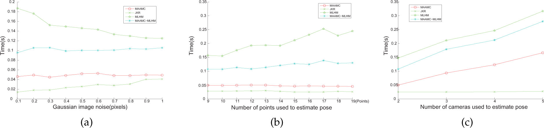
Experimental results for average time consumption
In order to evaluate the multi-camera algorithms' robustness, we also inspected the disturbance introduced by a small calibration error of the multi-camera system. The experiment was carried out by adding Gaussian noise to the parameters of the principal point (U0, V0) of each camera, the relative translation vector and the rotation angles, separately. The Gaussian noise magnitudes in U0, V0 were 2.5 pixels, and 10 mm for all three translation orientations, and 10 degrees for all three angles correspondingly. The viewing angles were set to be large. The 3D referenced points and cameras were placed in the same manner as in the first experiment. The pose estimation target-point was also set with a ground true value (430,760,200). We executed the estimation 50 times for each noised U0, V0, the relative translation vector T and the relative rotation R. The average results are shown in figure 5.
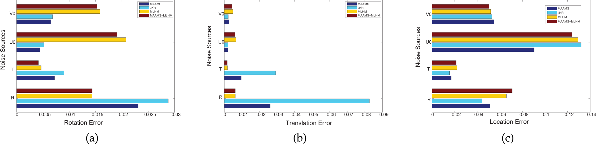
Simulation experiment results introducing a small calibration error. (a),(b) and (c) show the rotation, translation and location errors of the four methods with noise on their U0, V0 and rigid rig (R, T). The x-coordinates of these three sub-figures are relative errors, which refer to the corresponding errors compared with the absolute values, such as the values of the rotation, translation and distance.
According to figure 5(a) and (b), we can see that the object space-minimum-based methods (e.g., MLHM, MAACM − MLHM) will give better pose estimations than the others in relation to the rigid rig with noise, and that they will also perform fewer pose estimations than the image error-minimum-based methods (e.g., MAACM) as concerns the noise U0 and V0. In addition, figure 5(c) illustrates that our MAACM will achieve the best robustness as regards the overall performance of localization.
4.1.3. Overall performance analysis of the simulation experiments
In the above simulation experiments, we have presented the performances of seven state-of-the-art pose estimation methods for various metrics. In this section, we try to present an objective analysis of our approach, in terms of both robustness and accuracy, and in comparing it with the other six methods. In our analysis, we use a comparable performance diagram to illustrate the performance of our method vs the other methods. The results are shown in figure 6. In figure 6, each row compares the performance of our MAACM and the other methods for various metrics: the red block means that MAACM achieves better performance with the current metrics, the green block means that MAACM achieves worse performance with the current metrics, and the block with the dotted pattern means that MAACM is indistinguishable from the other methods.

Overall performance comparison of MAACM with other methods
The results in figure 6 illustrate that MAACM can achieve better performances for most of the metrics when compared to those methods obtaining poses simultaneously. As concerns the comparison between MAACM and RPP, it seems that RPP may be superior to our MAACM. We further consider that the reason why may be because RPP could search more possible intervals of camera poses without the constraint of rigs among the cameras during the optimization. Accordingly, we carried out another comparison between RPP and SAACM, which is our solution for MAACM when there is only one camera. The results are shown in figure 7, and they illustrate that our SAAMC may be superior to RPP. Thus, our approach is better as regards comprehensive performance under varied conditions and will be appropriate for implementation in applications requiring real-time and robust pose estimation, such as augmented reality and robots, etc.

Overall performance comparison of SAACM with RPP
4.2 Real case experiments
We also carried out comparative experiments using real image data. In these experiments, we built a miniature multi-camera system with two Toshiba Teli cameras, as shown in figure 8(left). Each camera was equipped with a 4 mm lens and operated at a resolution of 640 × 480. In the experiments, there were eight green referenced points placed on the ping-pong table and one static table tennis ball as a target point, as shown in figure 8(right). We randomly placed the cameras of the system and obtained their translation poses using the methods described above. Next, we computed the positions of the table tennis ball via the pose estimated by the different methods. The true positions of the table tennis ball were obtained via a 3D Micro-hite DCC coordinate-measuring machine (CCM) 9 . There were 12 random positions for the translation pose estimation and ball location - at each position, we executed each method 200 times and removed the maximum and minimum of each method. The final output results were the average of the remaining data. The experimental results are shown in figure 9. Figure 9 shows that MAAMC can achieve the highest location precision among all the methods and that it is also consistently more stable than the others.

Hardware(left) and software(right) of the multi-camera system used for real case experiments. In the right-hand figure, the upper-left view shows the 3D pose of the multi-camera system in the virtual environment, while the lower views show the images from the system and the upper-right view shows the detailed 6DOF poses.

Localization experimental results in the ping-pong robot vision system with different methods - the x-coordinate is the ratio of the distance error compared with the absolute distance
4.3 Practical implementation in ping-pong robots
The method presented in this article was originally motivated by our humanoid ping-pong robot project, which uses a multiple camera system to guide the robot arms during ping-pong games. We thus use the hardware described in Section 4.2 as the on-board vision system of the humanoid ping-pong robot. As concerns the vision system in the ping-pong robot, there are two main challenges in pose estimation due to the shaking of the robot. Firstly, there are few referenced points in this system, and the referenced 3D points are all located in the plane of the table. There are normally fewer than 10 correspondences, and so the vision system needs to estimate its pose and calculate the coordinates of the balls in the referenced point's coordinates with high accuracy using only a few coplanar points. Secondly, the vision system can be deployed at any angle relative to the ping-pong table, and so it may be placed in some locations with small viewing angles, which will greatly affect the accuracy of the pose estimation.
We implemented MAAMC in our humanoid ping-pong robot system [31]. In contrast to other ping-pong ball robots [32], we designed a 7DOF robot arm - which is very similar to a human arm - to play ping-pong.
The two-camera system as described in Section 4.2 tracks the ping-pong ball and generates its traces while playing. Figure 10 (right) shows the accuracy of the trace estimated by our method. The blue points show the true positions in this trace, which were obtained using an additional high-speed camera system with 500 frames/s working offline, while the white points show the trace estimated by our method in real-time 10 .

Left: the camera pose in our ping-pong robot system. Right: the trace obtained by our method (white) compared with the true trace (blue).
5. Conclusion
In this paper, we presented an efficient and robust pose estimation algorithm for multi-camera systems which can obtain 6DOF poses for all the cameras using only a few coplanar points simultaneously. Large-scale simulation experiments have shown that this algorithm can be more robust than the classical iterative pose estimation algorithm in both small- and large-angle viewing conditions. Practical experiments also showed that this method is more accurate and robust.
Hence, our method is especially suitable for implementation in tasks where there may be various poses for the cameras, including ill-condition or relatively small angles of viewing.
Footnotes
6. Acknowledgements
This research is based upon work supported in part by the National Science Foundation of China (61173123, 61203324, 61473258) and the Natural Science Foundation of Zhejiang (LR13F030003).
1
Here, we only need to estimate one representative pose of the multi-camera system - any other poses of any other camera may be obtained by transforming with the known orientations and translations existing between each camera.
2
Most approaches provide only 5DOF motion, and the scale of translation cannot be recovered. As such, we call our method ‘absolute pose estimation’.
4
In the following experiments, we use red lines to represent those pose estimation methods from coplanar points.
5
In the following experiments, we use green lines to represent those pose estimation methods from non-coplanar points.
6
In the following experiments, we use blue lines to represent this method.
7
In the following experiments, the unit for distance for a coordinate is mm.
8
In this experiment, we employed a very simple location method that extracts lines from each camera with two points - the image point of the object and the optic centre-point of each camera - and then calculated the centre of those lines as the position of the target.