Sage Journals: Discover world-class research

Abstract

The stiffness controller proposed by Salisbury is an interaction control strategy designed to achieve a desired form of static behavior as regards the interaction of a robot manipulator with the environment. The main idea behind this approach is the simulation of a multidimensional linear spring - or linear elastic material - using the difference between the actual position of the end-effector and a constant position (relaxed point), multiplied by a constant stiffness matrix. In this paper, this idea is generalized with the objective of proposing a controller structure that includes a family of stiffness models based on the idea of linear elastic materials. The new controller structure also includes a damping term in order to have control over energy dissipation, as well as a term added for the purpose of compensating the gravity forces of the links. The stability analysis of the proposed controller was performed in the Lyapunov sense. The new stiffness controller is presented as a case study and compared to other cases, such as the Salisbury controller (Cartesian PD) and the tanh-tanh controller. Experimental results using a three degrees-of-freedom direct-drive robot for the evaluation of controllers in a constrained motion task are presented.

Keywords

Interaction control Stiffness control Direct-drive robot

1. Introduction

Presently, robotic systems are extensively applied in many areas, including industry, medical applications (such as rehabilitation and surgery), and the exploration of dangerous or inaccessible environments for humans, etc. [1]. These applications can be classified in two groups in terms of interaction with the environment: if the robot executes tasks where there is no interaction with the environment, then the application belongs to an unconstrained-motion category; however, if there exists interaction, then the application corresponds to a constrained-motion category. Among the typical applications of unconstrained motion in industry, we might mention painting and laser cutting, etc.; meanwhile, among the industrial applications in which a constrained motion is needed, we might consider polishing, drilling, deburring machining and assembly, etc. In these applications, the control of interaction forces for the successful execution of the interaction tasks is crucial [2, 3]. In interaction tasks, the manipulator encounters environmental constraints and the interaction forces are not negligible [4].

Many researchers have been working on creating new schemes of the active interaction control of robot manipulators. There exist different approaches to the interaction control of robot manipulators, which can be classified as direct or indirect methods. Direct methods involve an explicit form representation of force-feedback, while in indirect methods force-feedback is not explicit but rather is regulated using the position of the end-effector. Among the most important direct interaction control approaches, we might consider explicit force control [5–7], hybrid force/position control [8–15] and parallel force/motion control [16, 17]. Meanwhile, among the most relevant indirect interaction control approaches, the stiffness control [18–22] and impedance control approaches [2, 4, 23–29] might be considered.

The explicit force-control approach [5] has been implemented in many ways. In this approach, the applied torques of the robot are commanded as a function of force error. The force error is referred to as the difference between the reference force and the actual interaction force, measured with a force/torque sensor. The main schemes in which explicit force control is implemented are: proportional control, integral control, proportional-integral control, proportional-derivative control and proportional-integral-derivative control [2, 7].

In the approach referred to as ‘hybrid force/position control’ [8], the workspace of the robot is divided into orthogonal directions that are constrained, either in terms of force or of position, and an appropriate force or position controller for each direction is designed.

'Parallel force/motion control’ is an interaction control approach that enables simultaneous movement control and force control [16]. The main idea is to use an inner-loop position control that works in parallel with a force-control loop. Conflicting situations between the position and force tasks are managed using a priority strategy: the force-control loop is designed to prevail over the position control loop. Recent works have included observers in order to acquire an estimation of velocity and to increase performance [17].

The approach referred to as ‘impedance control’ is based on the control of the relationship between the interaction force and positioning errors resulting from this force. The dynamic interaction between the manipulator and its environment can be regulated and controlled by changing its mechanical impedance. The impedance control introduced by Hogan [4] presents a general and unified approach to implement, in a robot manipulator, an impedance controller and generate a linear mass-spring-damper closed-loop system. Based on this approach, several control schemes have been developed for interaction control. Among them, the literature on robotics cites approaches like robust nonlinear impedance control [23], hybrid impedance control (HIC) [30] (which is a combination of impedance control and hybrid position/force control), adaptive impedance control (which considers parametric uncertainties in the robot model) [31], and an adaptive version of HIC [32] (which is used to compensate for parametric uncertainties in the robot model). Recent control schemes have been developed based on inverse-dynamics for dynamic compensation [28], yielding a PD-type control structure of the impedance error [27], which is useful for unconstrained and constrained motion; these approaches have been tested on a two-degrees-of-freedom direct-drive robot, and they present better performance than Hogan's impedance approach, both in relation to path-following tasks in unconstrained movement and in the case of interaction tasks.

The stiffness control proposed by Salisbury [18] is an interaction control approach designed to achieve the desired static behaviour of the interaction of a robot manipulator with the environment [4]. In this context, it is essentially a proportional-derivative (PD) position controller, with position and velocity feedback gains adjusted in order to obtain different apparent impedances. The stiffness control has been implemented in different schemes. Among them, in [19] an approach based on variable stiffness - referred to as a ‘self-controlled stiffness function’ - which is used for unknown environments is presented; [20] presents an approach based on adaptive stiffness characteristics for interacting with unknown environments; in [22], new sufficient stability conditions for stiffness control based on a Lyapunov-Hamiltonian function are presented. In this case, the stiffness control is used for robot-aided rehabilitation.

The original idea of stiffness control [18] concerned the simulation of a multidimensional linear spring, using the difference between the position of the end-effector and a constant position, multiplied by a constant matrix referred to as a ‘stiffness matrix'. In this context, the stiffness control reproduces the behaviour of a linear elastic material. This behaviour can be generalized by simulating a general elastic material using the stiffness matrix and a variable term defined as the difference between the actual and a constant position, which is considered as the relaxed position. In this paper, a new structure of stiffness control designed for static behaviour using a well-defined mathematical structure is presented. The proposed controller includes a damping term in order to control the dissipation of energy.

The Salisbury controller, associated with Cartesian control, is widely cited in the literature [1, 33]. However, no controller family structure, as proposed herein, has been reported for Cartesian space control, specifically in the context of stiffness control. Furthermore, it is important to note that similar structures have been reported in the case of joint space control. Moreover, the stability analysis for this control approach is usually performed using linear system techniques, and in the few papers that use a Lyapunov approach, such an analysis is performed in the joint space. In this case, we take advantage of the properties of the model in Cartesian space in order to demonstrate asymptotic stability. The advantage of this structure is that it results in a large number of control schemes that meet the characteristics of the proposed family.

This paper is organized as follows. In Section 2, a new family of stiffness regulators, their stability analysis in the Lyapunov sense, and a few case studies of stiffness regulators members, are presented. In Section 3, the platform used in the experiments and the experimental evidence of the aforementioned case studies are presented. Finally, conclusions are presented in Section 4.

2. A new family of stiffness regulators and dissipative injection

In this section, the control problem is formulated in Cartesian-space - for the purpose of clarity, the relationship between the well-known joint space dynamic model and the dynamic model of the end-effector in Cartesian-space is reviewed.

2.1 A dynamic model of robot manipulators

The dynamic analysis of the robot arm determines a relationship between the joint torques/forces applied by the actuators and the motion of the robot. This motion is described in terms of the joint positions, velocities and accelerations of the robot arm as a function of time. The dynamic model of a robot manipulator, in the joint space, is given by,

τ - J^{T} (q) f_{e} = M (q) \ddot{q} + C (q, \dot{q}) \dot{q} + g (q) + f (q)

(1)

where $q ∊ ℝ^{n}$ is the vector of joint displacements, $\dot{q} ∊ ℝ^{n}$ is the vector of joint velocities, $\ddot{q} ∊ ℝ^{n}$ is the vector of joint accelerations, $M (q) ∊ ℝ^{n \times n}$ is the symmetric positive definite manipulator inertia matrix, $C (q, \dot{q}) ∊ ℝ^{n \times n}$ is the matrix of centripetal and Coriolis torques, and $g (q) ∊ ℝ^{n}$ is the vector of gravitational torques obtained as the gradient of the robot total potential energy $U (q)$ . $f (\dot{q}) ∊ ℝ^{n}$ is the friction torque vector. In this paper, the common viscous friction model, i.e., $f (q) = B \dot{q}$ , where B is a diagonal matrix of viscous coefficients, is considered. Moreover, $τ ∊ ℝ^{n}$ is the vector of applied generalized forces/torques, while the external torques are given by the term J^T (q) f_e, where f_e denotes the vector of force and moment exerted by the end-effector on the environment.

Consider the forward kinematics map $x = h (q) ∊ ℝ^{m}$ . The dynamic model of robot manipulators (1) can be expressed in Cartesian space by using a coordinate change. It is necessary to consider the relationship between joint velocities and the end-effector Cartesian velocities $\dot{x} = J (q) \dot{q} ∊ ℝ^{m}$ , where $J (q) ∊ ℝ^{m \times n}$ is the Jacobian matrix. A relationship exists between the applied forces f_χ in Cartesian space at the end-effector and the applied torques Τ in the joints. This relationship is referred to as the Jacobian transposed controller’ [34], introduced by Takegaki and Arimoto, and is given by,

τ = J^{T} (q) f_{χ}

(2)

where

f_{χ} - f_{e} = M_{χ} \ddot{x} + C_{χ} \dot{x} + g_{χ} + f_{f χ}

(3)

The equation (3) is referred to as the ‘Cartesian dynamic model', which is valid only if the robot arm is away from kinematic singularities. The Cartesian dynamic model can be described in terms of the joint space dynamic model and the Jacobian matrix as,

\begin{matrix} M_{χ} = J^{- T} (q) M (q) J^{- 1} (q) \\ C_{χ} = J^{- T} (q) C (q, \dot{q}) J^{- 1} (q) - M_{χ} \dot{J} (q) J^{- 1} (q) \\ g_{χ} = J^{- T} (q) g (q) \\ f_{f χ} = B_{χ} \dot{x} \end{matrix}

$\dot{J} (q) = d J (q) / d t$ , while $J^{- T} (q) = {[J^{- 1} (q)]}^{T}$ and B_x = J^−T (q)B J⁻¹(q).

In the case of a kinematically redundant manipulator, i.e., with a non-square Jacobian matrix, a dynamically consistent, generalized inverse of the Jacobian [35] can be adopted as,

J^{†} (q) = J^{T} (q) {[J (q) J^{T} (q)]}^{- 1}

(4)

which is referred to as the ‘right pseudoinverse'. If J(q) is square, the pseudoinverse (4) is reduced to the standard inverse Jacobian matrix J⁻¹(q). Without loss of generality, in this paper a square Jacobian matrix is considered, i.e., m=n.

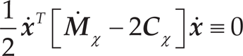
The Cartesian dynamic model (3) has important properties that are useful in control problems, the most important ones being,

Property 1 The matrix M_χ is a symmetric, positive definite matrix.

\begin{matrix} M_{χ} > 0, & M_{χ} = M_{χ}^{T} \end{matrix}

(5)

Property 2 Matrix M_χ is upper- and lower-bounded by

λ_{m i n} {M_{χ}} I \leq M_{χ} \leq λ_{m a x} {M_{χ}} I

(6)

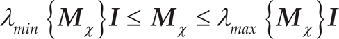
where λ_min, λ_max stands for the minimum and maximum eigenvalues of matrix M_χ.

Property 3 Since ${\dot{M}}_{χ} = C_{χ} + C_{χ}^{T}$ , the matrix ${\dot{M}}_{χ} - 2 C_{χ}$ is skew-symmetric, i.e.,

\frac{1}{2} {\dot{x}}^{T} [{\dot{M}}_{χ} - 2 C_{χ}] \dot{x} \equiv 0

(7)

Once the principal properties and the relationship between the Cartesian space and the joint space dynamic models are defined, it is possible to define a control problem and a proposed solution.

2.2 Defining a control problem

In mechanics, Hooke's law of elasticity is a model that states that the extension of a spring is in direct proportion to the load applied to it. Many materials comply with this law so long as the load does not exceed the material's elastic limit. Materials for which Hooke's law is a valid approximation are known as linear-elastic or “Hookean” materials. Hooke's law, in simple terms, states that strain is directly proportional to stress.

The most commonly encountered form of Hooke's law is the spring equation, which relates the force exerted by a spring to the stretched distance by using a spring constant k, measured in terms of force per length. Mathematically, Hooke's law states that

f (x) = - k (x - x_{0})

(8)

where x denotes the actual position of the spring's end while x₀ denotes its relaxed position, f(x) is the restoring force exerted by the spring on that end, and k is a scalar constant referred to as the spring constant. The negative sign indicates that the force exerted by the spring is in direct opposition to the direction of displacement. It is designated as a restoring force, as it tends to restore the system to its relaxed position. It is important to notice that the potential energy stored in the spring is given by $U (k, x, x_{0}) = \frac{1}{2} k {(x - x_{0})}^{2}$ .

For a robot arm, whose movements are typically in 3D space, the behaviour of a spring in the end-effector can be reproduced by considering the following expression, [18], which represents the model of a multidimensional spring or linear elastic material,

f_{χ} = - K (x - x_{d})

(9)

where x_d∊ⁿ denotes the relaxed position of the spring in the n-dimensional workspace, while x_d∊ⁿ denotes the actual position of the end-effector, or the virtual spring's end. K∊^nxn is known as the ‘stiffness matrix'. In this case, the artificial potential energy stored in the virtual spring is given by $U_{a} (K, x, x_{d}) = \frac{1}{2} {(x - x_{d})}^{T} K (x - x_{d})$ .

The multidimensional Hook model (9) describes the behaviour of an n-dimensional linear spring - it is important to note that this model belongs to a particular class of spring models. In particular, this model describes a linear spring with no physical constraint, i.e., expression (9) models a linear spring that can be stretched or compressed in any direction with any displacement. The focus of this paper is to extend this idea by considering a multidimensional spring model by using Hook's law in a generalized function. The most important elements used to describe the model are the following: a constant spring matrix, denoted by $K_{p} ∊ ℝ^{n \times n}$ , and a displacement variable denoted by $\tilde{x} ∊ ℝ^{n}$ and defined as $\tilde{x} = x_{d} - x$ .

The expression for our generalized virtual spring model is given by

f_{χ} = \nabla U_{a} (K_{p}, \tilde{x})

(10)

this model is written using a notation that makes it easy to relate to the potential energy given by $U_{a} (K_{p}, \tilde{x})$ .

This paper addresses an indirect interaction control approach, referred to as an indirect stiffness control approach, which will be related to the Cartesian robot-control structure. In such a control structure, a force modelled in (10) - in stable state - is applied with the end-effector to a fixed environment (restricted motion); the force is indirectly manipulated by controlling the position of the end-effector with respect to a constant given position which serves as the relaxed point of the virtual spring model.

The aforementioned control problem can be defined, indirectly, in terms of a Cartesian position-regulation problem for unconstrained motion, which consists of finding f_χ in order to accurately achieve a desired constant position x_d starting from a near-initial condition x(0). In more formal terms, in the case of unconstrained motion, the control objective consists of finding f_χ such that

\lim_{t \to \infty} \tilde{x} (t) = 0

(11)

where $\tilde{x} ∊ ℝ^{n}$ stands for the Cartesian position-error vector or position error - in more simple terms - and is defined by

\tilde{x} = x_{d} - x (t)

(12)

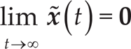
where x _d is defined as stated above.

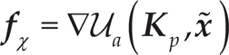
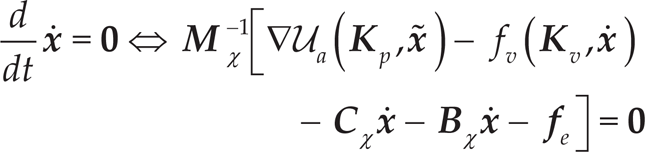
If the manipulator performs a constrained motion, it is clear that it is not possible to achieve the control objective (11). In this case, in a similar manner to that of the classical stiffness control [18] designed for static behaviour, the control objective for a constrained motion consists of applying a force to the environment with the end-effector at the contact point, given by

\lim_{t \to \infty} f_{e} = \nabla U_{a} (K_{p}, {\tilde{x}}_{E})

(13)

where ${\tilde{x}}_{E} = x_{d} - x_{E}$ . In this case, x_E denotes a constant vector representing the position achieved by the end-effector as $t \to \infty$ .

Proposition. In order to achieve the control objective for unconstrained motion given by (11), and in order to satisfy our definition of an indirect stiffness-control approach with the control objective for constrained motion given in (13), a new structure for controllers is proposed as follows,

f_{χ} = \nabla U_{a} (K_{p}, \tilde{x}) - f_{v} (K_{v}, \dot{x}) + g_{χ}

(14)

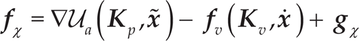
The proposed control (14) associates the artificial potential energy $U_{a} (K_{p}, \tilde{x})$ , the energy-shaping of which leads to $\nabla U_{a} (K_{p}, \tilde{x})$ , and a damping-injection term $f_{v} (K_{v}, \dot{x})$ . The term $\nabla U_{a} (K_{p}, \tilde{x})$ corresponds to a virtual generalized spring model, the second term $f_{v} (K_{v}, \dot{x})$ is a dissipative function, where K_v is referred to as the ‘diagonal damping matrix', while the last term represents the gravity forces. It is important to note that at least partial knowledge of the dynamic model of the manipulator is needed in order to implement the controller, i.e., in order to compute g_χ, both the vector of gravity torques g ( q ) and the Jacobian matrix J ( q ) are required.

Assuming that x_d is a constant vector, the equation that describes the closed-loop system can be represented in terms of the state vector ${[\begin{matrix} {\tilde{x}}^{T} & {\dot{x}}^{T} \end{matrix}]}^{T} ∊ ℝ^{2 n}$ , which is obtained by combining equations (3) and (14), and is given by

\frac{d}{d t} [\begin{matrix} \tilde{x} \\ \dot{x} \end{matrix}] = [\begin{matrix} - \dot{x} \\ M_{χ}^{- 1} Ψ_{χ} \end{matrix}]

(15)

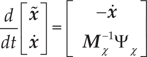
where

Ψ_{χ} = \nabla U_{a} (K_{p}, \tilde{x}) - f_{v} (K_{v}, \dot{x}) - C_{χ} \dot{x} - B_{χ} \dot{x} - f_{e}

In the robotics literature, a simple but significant model of contact [36] is widely used. In this case, a decoupled, elastically compliant environment is considered $f_{e} ∊ ℝ^{n}$ , which is described by the following model,

f_{e} = K_{e} (x - x_{e})

(16)

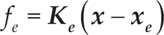
where $K_{e} ∊ ℝ^{n \times n}$ is referred to as the ‘stiffness matrix of the environment', the term x_e denotes the contact position with the environment, and x denotes the actual position of the end-effector.

2.3 Lyapunov stability analysis

In order to study the existence of the equilibrium point of the system (15), an analysis is performed under the following conditions, [(i)]

1.
For design purposes, we assume that

$\nabla U_{a} (K_{p}, \tilde{x}) = 0 \Leftrightarrow \tilde{x} = 0, K_{p} > 0$
(17)

$f_{v} (K_{v}, \dot{x}) = 0 \Leftrightarrow \dot{x} = 0, K_{v} > 0$
(19)

2.
It is true that

$\begin{array}{l} C_{χ} \dot{x} = 0 \Leftrightarrow \dot{x} = 0 \\ B_{χ} \dot{x} = 0 \Leftrightarrow \dot{x} = 0 \end{array}$
(19)

The first condition for the existence of the equilibrium point is given by

$\frac{d}{d t} \tilde{x} = 0 \Leftrightarrow \dot{x} = 0$
(20)

which implies that x is constant when condition (20) is true. This constant vector will be denoted as x_E, and as such a constant vector exists, ${\tilde{x}}_{E} = x_{d} - x_{E}$ .

The second condition is given by

$\begin{array}{l} \frac{d}{d t} \dot{x} = 0 \Leftrightarrow M_{χ}^{- 1} [\nabla U_{a} (K_{p}, \tilde{x}) - f_{v} (K_{v}, \dot{x}) \\ - C_{χ} \dot{x} - B_{χ} \dot{x} - f_{e}] = 0 \end{array}$
(21)

Considering that $M_{χ} > 0 \Rightarrow \exists M_{χ}^{- 1} > 0$ , and given condition (20), then by considering (18) and (19), we obtain

$f_{e} = \nabla U_{a} (K_{p}, \tilde{x})$
(22)

which is consistent with Newton's third law on steady states.

It is important to analyse the expression (22) and interpret it correctly. If the interaction force does not exist, then $f_{e} = 0 = \nabla U_{a} (K_{p}, \tilde{x})$ , and considering (17) we obtain $\tilde{x} = 0$ ; in this case, the origin is an equilibrium point of the system (15). If the interaction force exists, it is given by $f_{e} = \nabla U_{a} (K_{p}, {\tilde{x}}_{E})$ ; hence, the equilibrium point of the system (15) is ${[\begin{matrix} {\tilde{x}}_{E}^{T} & 0^{T} \end{matrix}]}^{T} ∊ ℝ^{2 n}$ .

The concern of this section is to perform the stability analysis in a Lyapunov sense for the system (15) when an interaction force exists, as the opposite case is trivial. We will proceed in a similar manner as Canudas et al, [35], who analyses the classical stiffness control approach with an equilibrium point out of the origin.

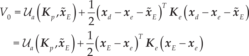
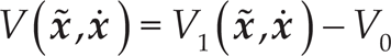
Consider the following Lyapunov-like function

$\begin{array}{l} V_{1} (\tilde{x}, \dot{x}) = \frac{1}{2} {\dot{x}}^{T} M_{χ} \dot{x} + U_{a} (K_{p}, \tilde{x}) \\ + \frac{1}{2} {(x_{d} - x_{e} - \tilde{x})}^{T} K_{e} (x_{d} - x_{e} - \tilde{x}) \\ = \frac{1}{2} {\dot{x}}^{T} M_{χ} \dot{x} + U_{a} (K_{p}, \tilde{x}) \\ + \frac{1}{2} {(x - x_{e})}^{T} K_{e} (x - x_{e}) \end{array}$
(23)

where the first and third terms are radially unbounded and positive definite - due to their quadratic form - and $U_{a} (K_{p}, \tilde{x})$ is proposed as a definite positive function in order to have the same properties as function $V_{1} (\tilde{x}, \dot{x})$ . For example, it is possible to propose $U_{a} (K_{p}, \tilde{x})$ in a quadratic form or otherwise, which is positive definite.

The minimum of $V_{1} (\tilde{x}, \dot{x})$ is obtained when the following conditions are met

$\begin{array}{l} \frac{\partial V_{1} (\tilde{x}, \dot{x})}{\partial \dot{x}} = M_{χ} \dot{x} = 0 \\ \frac{\partial V_{1} (\tilde{x}, \dot{x})}{\partial \tilde{x}} = \nabla U_{a} (K_{p}, \tilde{x}) - \underset{f_{e}}{\underset{︸}{K_{e} (x - x_{e})}} = 0 \end{array}$

hence, the minimum $V_{1} (\tilde{x}, \dot{x})$ is obtained at ${[\begin{matrix} {\tilde{x}}_{E}^{T} & 0^{T} \end{matrix}]}^{T} ∊ ℝ^{2 n}$ , i.e., at the equilibrium point. As such, V₀ is given as

$\begin{array}{l} V_{0} = U_{a} (K_{p}, {\tilde{x}}_{E}) + \frac{1}{2} {(x_{d} - x_{e} - {\tilde{x}}_{E})}^{T} K_{e} (x_{d} - x_{e} - {\tilde{x}}_{E}) \\ = U_{a} (K_{p}, {\tilde{x}}_{E}) + \frac{1}{2} {(x_{E} - x_{e})}^{T} K_{e} (x_{E} - x_{e}) \end{array}$
(24)

For the stability analysis of the equilibrium point ${[\begin{matrix} {\tilde{x}}_{E}^{T} & 0^{T} \end{matrix}]}^{T} ∊ ℝ^{2 n}$ of the system (15), the following Lyapunov candidate function is considered,

$V (\tilde{x}, \dot{x}) = V_{1} (\tilde{x}, \dot{x}) - V_{0}$
(25)

where $V_{1} (\tilde{x}, \dot{x})$ and V₀ are given in (23) and (24) respectively.

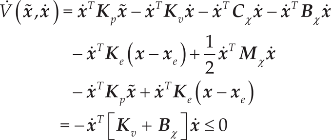
The time derivative of the Lyapunov candidate function (25) along the trajectories of the closed-loop system (15) is given as follows,

$\begin{array}{l} \dot{V} (\tilde{x}, \dot{x}) = {\dot{x}}^{T} M_{χ} \ddot{x} + \frac{1}{2} {\dot{x}}^{T} M_{χ} \dot{x} - {\dot{x}}^{T} \nabla U_{a} (K_{p}, \tilde{x}) \\ + {\dot{x}}^{T} K_{e} (x - x_{e}) \end{array}$
(26)

Thus, by substituting $M_{χ} \ddot{x} = \nabla U_{a} (K_{p}, \tilde{x}) - f_{v} (K_{v}, \dot{x}) - C_{χ} \dot{x} - B_{χ} \dot{x} - K_{e} (x - x_{e})$ from the closed-loop equation (15), and using Property 3 with ${\dot{x}}^{T} [\frac{1}{2} {\dot{M}}_{χ} - C_{χ}] \dot{x} = 0$ , we get

$\begin{array}{l} \dot{V} (\tilde{x}, \dot{x}) = {\dot{x}}^{T} \nabla U_{a} (K_{p}, \tilde{x}) - {\dot{x}}^{T} f_{v} (K_{v}, \dot{x}) - {\dot{x}}^{T} C_{χ} \dot{x} - {\dot{x}}^{T} B_{χ} \dot{x} \\ - {\dot{x}}^{T} K_{e} (x - x_{e}) + \frac{1}{2} {\dot{x}}^{T} M_{χ} \dot{x} - {\dot{x}}^{T} \nabla U_{a} (K_{p}, \tilde{x}) \\ + {\dot{x}}^{T} K_{e} (x - x_{e}) \\ = - {\dot{x}}^{T} f_{v} (K_{v}, \dot{x}) - {\dot{x}}^{T} B_{χ} \dot{x} \leq 0 \end{array}$
(27)

where ${\dot{x}}^{T} f_{v} (K_{v}, \dot{x}) > 0$ is designed as a sigmoid dissipative term, and B_χ = J^−T BJ₋₁ > 0 due to B>0. Since $\dot{V} (\tilde{x}, \dot{x})$ is a negative, semi-definite function - in agreement with Lyapunov's direct method - the control law yields a stable closed-loop system.

Since the closed-loop equation (15) describes an autonomous nonlinear system, the use of LaSalle's theorem [37] is a valid alternative to analyse the asymptotic stability of the equilibrium point.

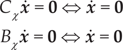
With this aim in mind, the set Ω is used

$\begin{array}{l} Ω = {ω ∊ ℝ^{2 n} : \dot{V} (ω) = 0} \\ = {ω = [\begin{matrix} \tilde{x} \\ \dot{x} \end{matrix}] ∊ ℝ^{2 n} : \dot{V} (\tilde{x}, \dot{x}) = 0} \\ = {\tilde{x} ∊ ℝ^{n}, \dot{x} = 0 ∊ ℝ^{n}} \end{array}$
(28)

Observe that $\dot{V} (\tilde{x}, \dot{x}) = 0$ if, and only if, $\dot{x} = 0$ . For a solution ω (t) to belong to Ω for all t ≥0, it is necessary and sufficient that x(t) = 0 for all t≥0. Therefore, it must also hold that $\ddot{x} (t) = 0$ for all t≥0. Taking this into account, we conclude from the closed-loop equation (15), followed by equation (21), that, if ω(t)∊Ω for all t≥0, then

$0 = M_{χ}^{- 1} [\nabla U_{a} (K_{p}, \tilde{x}) - f_{e}]$
(29)

which means that $\tilde{x} = {\tilde{x}}_{E}$ for all t≥0. Thus, ${[\begin{matrix} \tilde{x} {(0)}^{T} & \dot{x} {(0)}^{T} \end{matrix}]}^{T} = {[\begin{matrix} {\tilde{x}}_{E}^{T} & 0^{T} \end{matrix}]}^{T} ∊ ℝ^{2 n}$ is the only initial condition in Ω for which ω(t)∊Ω for all t ≥0. As such, according to LaSalle's theorem, this is enough to guarantee the asymptotic stability of the equilibrium point ${[\begin{matrix} {\tilde{x}}^{T} & {\dot{x}}^{T} \end{matrix}]}^{T} = {[\begin{matrix} {\tilde{x}}_{E}^{T} & 0^{T} \end{matrix}]}^{T} ∊ ℝ^{2 n}$ .

As a result, the equilibrium point ${[\begin{matrix} {\tilde{x}}_{E}^{T} & 0^{T} \end{matrix}]}^{T}$ is asymptotically stable, i.e.,

$\begin{array}{l} \lim_{t \to \infty} \tilde{x} (t) = {\tilde{x}}_{E} \Rightarrow \lim_{t \to \infty} f_{e} = \nabla U_{a} (K_{p}, \tilde{x}_{E}) \\ \lim_{t \to \infty} \dot{x} (t) = 0 \end{array}$

As such, the control objective for the indirect stiffness control approach is achieved. Further details are given in the Appendix, where the boundedness of the state-equation solution is studied.
2.4 Case studies

Several controllers can be generated by using the proposed structure (14), and some examples are given below.

2.4.1 PD-type controller structure

The PD Cartesian position controller (Salisbury's stiffness controller) belongs to the family of stiffness controllers with dissipative terms, which are given in (14). The structure of the PD regulator can be formed by using a linear spring model $\nabla U_{a} (K_{p}, \tilde{x}) = K_{p} \tilde{x}$ , and is given by

f_{χ} = K_{p} \tilde{x} - K_{v} \dot{x} + g_{χ}

(30)

In order to perform the stability analysis of the dynamic system given in (15) for this controller, the following Lyapunov function candidate is used,

V (\tilde{x}, \dot{x}) = V_{1} (\tilde{x}, \dot{x}) - V_{0}

(31)

where

\begin{array}{l} V_{1} (\tilde{x}, \dot{x}) = \frac{1}{2} {\dot{x}}^{T} M_{χ} \dot{x} + \frac{1}{2} {\tilde{x}}^{T} K_{p} \tilde{x} \\ + \frac{1}{2} {(x - x_{e})}^{T} K_{e} (x - x_{e}) \end{array}

(32)

V_{0} = \frac{1}{2} {\tilde{x}}_{E}^{T} K_{p} {\tilde{x}}_{E} + \frac{1}{2} {(x_{E} - x_{e})}^{T} K_{e} (x_{E} - x_{e})

(33)

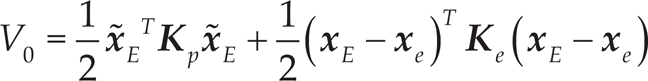
In this case, V₀ was obtained in a similar way to the general case presented above.

The time-derivative of the Lyapunov candidate function (31) along the trajectories is

\begin{array}{l} \dot{V} (\tilde{x}, \dot{x}) = {\dot{x}}^{T} K_{p} \tilde{x} - {\dot{x}}^{T} K_{v} \dot{x} - {\dot{x}}^{T} C_{χ} \dot{x} - {\dot{x}}^{T} B_{χ} \dot{x} \\ - {\dot{x}}^{T} K_{e} (x - x_{e}) + \frac{1}{2} {\dot{x}}^{T} M_{χ} \dot{x} \\ - {\dot{x}}^{T} K_{p} \tilde{x} + {\dot{x}}^{T} K_{e} (x - x_{e}) \\ = - {\dot{x}}^{T} [K_{v} + B_{χ}] \dot{x} \leq 0 \end{array}

(34)

In order to study the asymptotic stability, it is possible to apply LaSalle's theorem in the region (28), where the unique invariant is ${[\begin{matrix} {\tilde{x}}^{T} & {\dot{x}}^{T} \end{matrix}]}^{T} = {[\begin{matrix} {\tilde{x}}_{E}^{T} & 0^{T} \end{matrix}]}^{T} ∊ ℝ^{2 n}$ .

2.4.2 Tanh-tanh-type controller structure

The tanh-tanh Cartesian controller structure reproduces the behaviour of a nonlinear virtual spring plus a saturated dissipative term. In Cartesian space, this controller represents a saturated PD regulator, but in the joint space this feature is not satisfied since the applied torques are not saturated. The structure of the tanh-tanh controller is given by

f_{χ} = K_{p} t a n h (\tilde{x}) - K_{v} t a n h (\dot{x}) + g_{χ}

(35)

where tanh(α) represents - using a simplified notation - a vectorial function given by

t a n h (α) = [\begin{matrix} \tanh (α_{1}) \\ ⋮ \\ \tanh (α_{n}) \end{matrix}]

(36)

for $α = \tilde{x}, \dot{x} ∊ ℝ^{n}$

Furthermore, the stability analysis can be carried out by selecting the following candidate Lyapunov function,

V (\tilde{x}, \dot{x}) = V_{1} (\tilde{x}, \dot{x}) - V_{0}

(37)

where

\begin{array}{l} V_{1} (\tilde{x}, \dot{x}) = \frac{1}{2} {\dot{x}}^{T} M_{χ} \dot{x} + \frac{1}{2} {(x - x_{e})}^{T} K_{e} (x - x_{e}) \\ + {[\begin{matrix} \sqrt{\ln {\cosh ({\tilde{x}}_{1})}} \\ ⋮ \\ \sqrt{\ln {\cosh ({\tilde{x}}_{n})}} \end{matrix}]}^{T} K_{p} [\begin{matrix} \sqrt{\ln {\cosh ({\tilde{x}}_{1})}} \\ ⋮ \\ \sqrt{\ln {\cosh ({\tilde{x}}_{n})}} \end{matrix}] \end{array}

(38)

\begin{array}{l} V_{0} = \frac{1}{2} {(x_{E} - x_{e})}^{T} K_{e} (x_{E} - x_{e}) \\ + {[\begin{matrix} \sqrt{\ln {\cosh ({\tilde{x}}_{E 1})}} \\ ⋮ \\ \sqrt{\ln {\cosh ({\tilde{x}}_{E n})}} \end{matrix}]}^{T} K_{p} [\begin{matrix} \sqrt{\ln {\cosh ({\tilde{x}}_{E 1})}} \\ ⋮ \\ \sqrt{\ln {\cosh ({\tilde{x}}_{E n})}} \end{matrix}] \end{array}

(39)

In this case, V₀ was obtained in a similar way to the general case presented above.

The time-derivative of the Lyapunov candidate function (37) along the trajectories is

\begin{array}{l} \dot{V} (\tilde{x}, \dot{x}) = {\dot{x}}^{T} K_{p} t a n h (\tilde{x}) - {\dot{x}}^{T} K_{v} t a n h (\dot{x}) - {\dot{x}}^{T} C_{χ} \dot{x} \\ - {\dot{x}}^{T} B_{χ} \tilde{x} - {\dot{x}}^{T} K_{e} (x - x_{e}) + \frac{1}{2} {\dot{x}}^{T} M_{χ} \dot{x} \\ - {\dot{x}}^{T} K_{p} t a n h (\tilde{x}) + {\dot{x}}^{T} K_{e} (x - x_{e}) \\ = - {\dot{x}}^{T} K_{v} t a n h (\dot{x}) - {\dot{x}}^{T} B_{χ} \tilde{x} \leq 0 \end{array}

(40)

Considering that K_v>0 is a diagonal matrix, note that ${\dot{x}}^{T} K_{v} t a n h (\dot{x}) = 0$ , if x=0 and ${\dot{x}}^{T} K_{v} t a n h (\dot{x}) > 0$ otherwise.

2.4.3 Reciprocal-quadratic-type controller structure

The reciprocal-quadratic (RQ) Cartesian controller is a new member of the family of indirect stiffness regulators, which reproduces the dynamic behaviour of a virtual nonlinear spring in addition to a dissipative term. Similar to the tanh-tanh structure, this controller represents a saturated-proportional/saturated-derivative regulator in Cartesian space, although the applied torques are not saturated in the joint space. The structure of the RQ-type controller, which was proposed while looking for a mathematical structure that would meet the properties of the stiffness control family, is given by (41). This control structure represents a control scheme that is inversely proportional to the position error. When the position error is large, the control provides a small applied torque, while when the position error is small, the torque will be within the operational range, as provided by a proper tuning of the controller gains. With these properties, the control scheme drives the position error to zero.

f_{χ} = K_{p} \frac{\tilde{x}}{1 + {\tilde{x}}^{2}} - K_{v} \frac{\dot{x}}{1 + {\dot{x}}^{2}} + g_{χ}

(41)

where the following vectorial function is described - using a simplified notation - as

\frac{α}{1 + α^{2}} = [\begin{matrix} \frac{α_{1}}{1 + α_{1}^{2}} \\ ⋮ \\ \frac{α_{n}}{1 + α_{n}^{2}} \end{matrix}]

(42)

for $α = \tilde{x}, \dot{x} ∊ ℝ^{n}$

Moreover, in order to carry out the stability analysis, the following candidate Lyapunov function is proposed,

V (\tilde{x}, \dot{x}) = V_{1} (\tilde{x}, \dot{x}) - V_{0}

(43)

where

\begin{array}{l} V_{1} (\tilde{x}, \dot{x}) = \frac{1}{2} {\dot{x}}^{T} M_{χ} \dot{x} + \frac{1}{2} {(x - x_{e})}^{T} K_{e} (x - x_{e}) \\ + {[\begin{matrix} \sqrt{\ln (1 + {\tilde{x}}_{1}^{2})} \\ ⋮ \\ \sqrt{\ln (1 + {\tilde{x}}_{n}^{2})} \end{matrix}]}^{T} K_{p} [\begin{matrix} \sqrt{\ln (1 + {\tilde{x}}_{1}^{2})} \\ ⋮ \\ \sqrt{\ln (1 + {\tilde{x}}_{n}^{2})} \end{matrix}] \end{array}

(44)

\begin{array}{l} V_{0} = \frac{1}{2} {(x_{E} - x_{e})}^{T} K_{e} (x_{E} - x_{e}) \\ + {[\begin{matrix} \sqrt{\ln (1 + {\tilde{x}}_{E 1}^{2})} \\ ⋮ \\ \sqrt{\ln (1 + {\tilde{x}}_{E n}^{2})} \end{matrix}]}^{T} K_{p} [\begin{matrix} \sqrt{\ln (1 + {\tilde{x}}_{E 1}^{2})} \\ ⋮ \\ \sqrt{\ln (1 + {\tilde{x}}_{E n}^{2})} \end{matrix}] \end{array}

(45)

In this case, V₀ was obtained in a similar way to the general case presented above.

The time-derivative of the Lyapunov candidate function (43) along the trajectories is

\begin{array}{l} \dot{V} (\tilde{x}, \dot{x}) = {\dot{x}}^{T} K_{p} \frac{\tilde{x}}{1 + {\tilde{x}}^{2}} - {\dot{x}}^{T} K_{v} \frac{\dot{x}}{1 + {\dot{x}}^{2}} - {\dot{x}}^{T} C_{χ} \dot{x} - {\dot{x}}^{T} B_{χ} \dot{x} \\ - {\dot{x}}^{T} K_{e} (x - x_{e}) + \frac{1}{2} {\dot{x}}^{T} M_{χ} \dot{x} \\ - {\dot{x}}^{T} K_{p} \frac{\tilde{x}}{1 + {\tilde{x}}^{2}} + {\dot{x}}^{T} K_{e} (x - x_{e}) \\ = - {\dot{x}}^{T} K_{v} \frac{\dot{x}}{1 + {\dot{x}}^{2}} - {\dot{x}}^{T} B_{χ} \dot{x} \leq 0 \end{array}

(46)

Considering that K_v>0 is a diagonal matrix, note that ${\dot{x}}^{T} K_{v} \frac{\dot{x}}{1 + {\dot{x}}^{2}} = 0$ if $x = 0$ , and ${\dot{x}}^{T} K_{v} \frac{\dot{x}}{1 + {\dot{x}}^{2}} > 0$ otherwise.

3. Experimental evidence

Experimental evidence of the performance of the proposed controllers was obtained using an anthropomorphic direct-drive robot which was designed and built at the Robotics laboratory of Benemérita Universidad Autónoma de Puebla (BUAP). The three-degrees-of-freedom robot, “Rotradi” (Figure 1), consists of three 6061 aluminium alloy order to drive the joints without gear reduction. The motors used in “Rotradi” comprise DM-1050A, DM-1150A and DM-1015B models from Parker Compumotor for the base and the shoulder and elbow joints, respectively. The servomotors are operated in torque mode, which means that the motor acts as a torque source and that they accept an analogue voltage as a reference for the torque signal. The features of the servo actuators are shown in Table 1. The robot system has a device designed for reading the encoders and generating the reference voltages, namely a motion control board from Precision MicroDynamics Inc. The control algorithms are written in the language C and run in real-time with a 2.5 ms sample period on a Pentium 1 computer running at 166 MHz.

Figure 1.

Experimental robot “Rotradi”

Table 1.

Robot arm servo actuators

Joint	Model	Max. Torque	Resolution [cpr]
1. Base	DM-1050	50	1,024,000
2. Shoulder	DM-1150A	150	1,024,000
3. Elbow	DM-1015B	15	1,024,000

A challenging task to which the controllers presented in this work can be applied involves engraving a metal surface using a drill mounted at the third link of the arm, as shown in Figure 1. The direct kinematics are helpful in describing the experimental results due to the fact that the proposed control structure is given in Cartesian space. The direct kinematics x of the robot used in the experiments are given as follows,

\begin{array}{l} x_{1} = (d_{2} + d_{3} + d_{z}) \cos (q_{1}) - (l_{3} + d_{x}) \sin (q_{1}) \sin (q_{2} + q_{3}) \\ - d_{y} \sin (q_{1}) \cos (q_{2} + q_{3}) - l_{2} \sin (q_{1}) \sin (q_{2}) \end{array}

(47)

\begin{array}{l} x_{2} = (d_{2} + d_{3} + d_{z}) \sin (q_{1}) + (l_{3} + d_{x}) \cos (q_{1}) \sin (q_{2} + q_{3}) \\ + d_{y} \cos (q_{1}) \cos (q_{2} + q_{3}) + l_{2} \cos (q_{1}) \sin (q_{2}) \end{array}

(48)

\begin{array}{l} x_{3} = d_{y} \sin (q_{2} + q_{3}) - (l_{3} + d_{x}) \cos (q_{2} + q_{3}) \\ - l_{2} \cos (q_{2}) \end{array}

(49)

where l₂ = l₃ = 0.45m represent the lengths of the second and third links, while d₂ = 0.15m and d₃ = 0.10m denote the lengths of the servos for the shoulder and elbow joints, respectively. In addition, d_x = 0.175m, d_y = − 0.03m and d_z = 0.05m represent the dimensions of the tool attached at the third link. As commented upon above, and in order to compute $g_{χ}$ , both the gravitational torque vector g (q) and the Jacobian matrix J (q) are required. The complete dynamic model of our experimental robot “Rotradi” is presented in [38].

The experiment was designed in order to evaluate the performance of all the aforementioned control schemes. This experiment consists of placing the robot at an initial configuration by using the joint control and then the Cartesian control is activated. The reference for the stiffness control is given in such a way that the interaction between the tool and the metal surface is ensured. The metal surface, consisting of an aluminium sheet, is placed on the force sensor in order to measure the interaction forces. At the same time, the sensor is fixed on a work table. The objective of the manoeuvre is to leave a mark on the metal surface of the metal sheet using a drill. The initial conditions are depicted in Figure 1.

The initial position for the end-effector was set at x(0) = 0.300 0.420-0.585 m, and the desired position was x_d = 0.300 0.420-0.688 m; furthermore, the work surface was placed - with respect to the robot - at a distance of approximately z_e = − 0.686m. Table 2 shows the gain matrices for all the control schemes. These values were selected based on the experience obtained while tuning the controllers in Cartesian space.

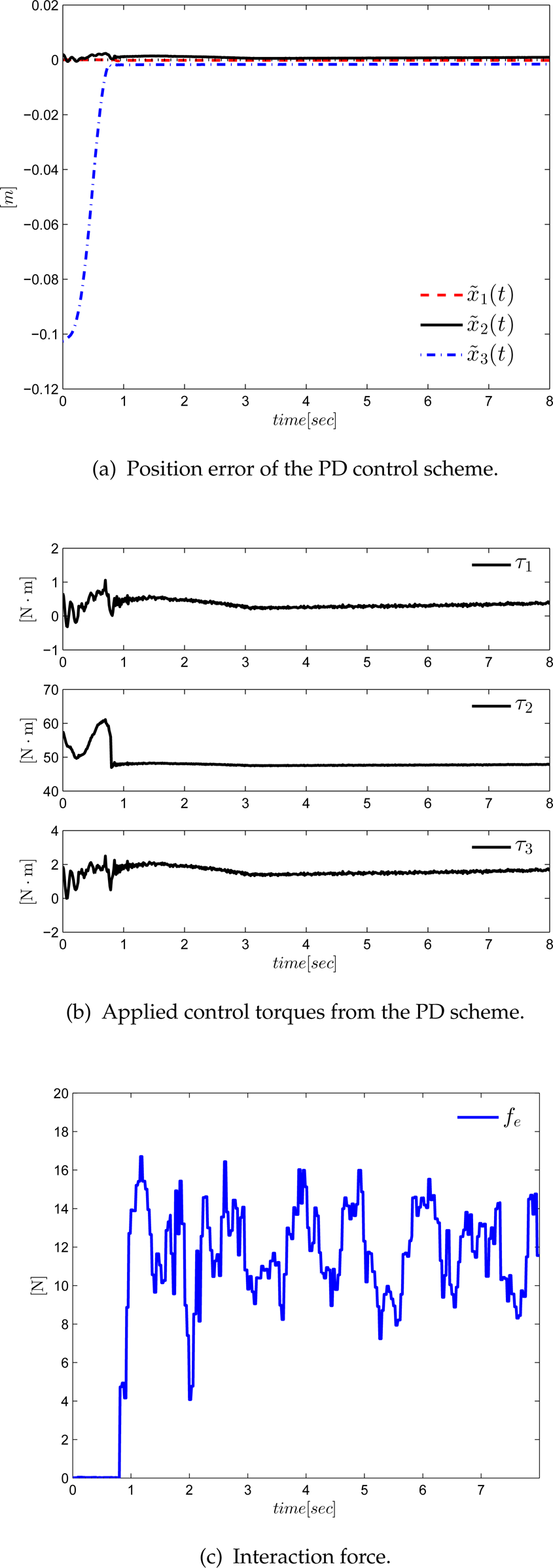
The results of all the control schemes are now presented. For each control scheme, the results regarding the position errors, the applied control torques and the interaction force, measured with the force sensor, are shown. It is worth mentioning that, in order to mark the surface, the experiments had to be performed with the drill turned on.

Table 2.

The gain matrix for all the control schemes

Control scheme	K_p	K_v
PD	diag(750.0,1150.0,750.0)	diag(15.0,15.0,40.0)
tanh	diag(750.0,1750.0,850.0)	diag(15.0,15.0,45.0)
RQ	diag (750.0,1750.0,800.0)	diag(15.0,15.0,45.0)

Figure 2.

Experimental evidence for the PD control scheme

Figure 3.

Experimental evidence for the tanh-tanh control scheme

The results of the PD control scheme are shown in figures 2(a), 2(b) and 2(c). The first figure shows that there exists an error in the x₃ direction, due to the interaction with the surface. The second figure shows that the applied torques are within the operational range. The last figure shows that the interaction force is noisy due to the vibration of the rotating tool.

Figure 4.

Experimental evidence for the RQ control scheme

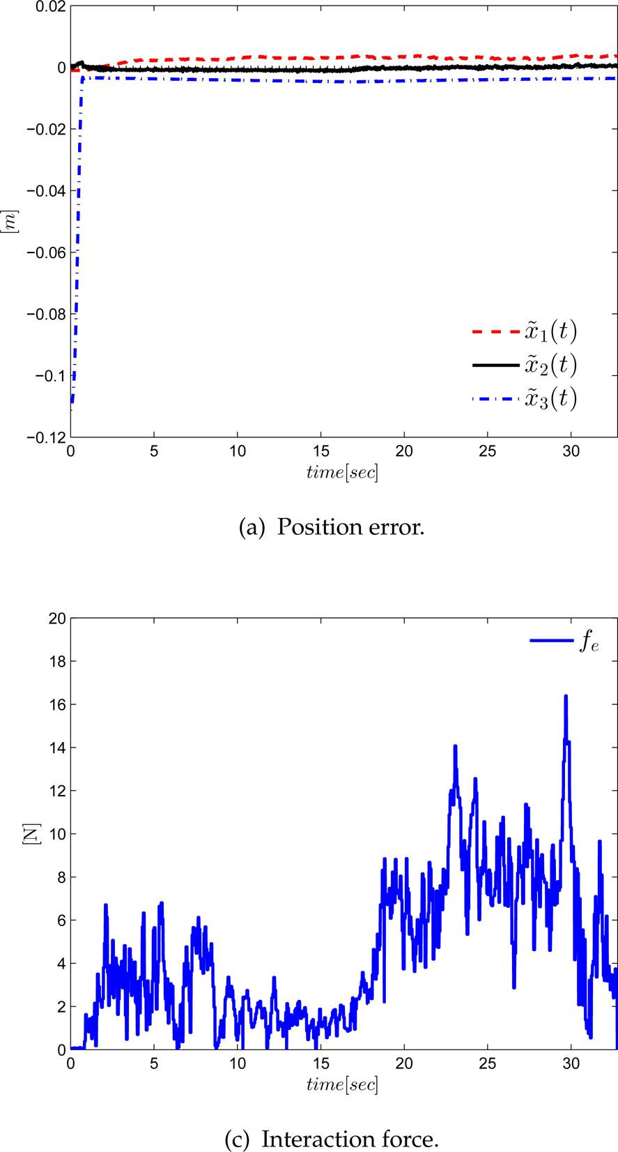
The results of the tanh-tanh control scheme are shown in Figures 3(a), 3(b) and 3(c). The results of the tanh-tanh scheme are similar to the e results of t n h he PD scheme.

The results of the RQ control scheme are shown in Figures 4(a), 4(b) and 4(c). The results of the RQ scheme are similar to the results of the two aforementioned control schemes.

The proportional and derivative gains were tuned, for each controller, by trial and error; in the experiments, these gains were empirically designed to seek the best time-response, without overshoot and with a minimum steady-state position error. From the experimental results, it can be seen that all the components of the position error, after a smooth transient, tend asymptotically to a small neighbourhood of zero. The response obtained with these controllers does not exhibit overshoot while also achieving fast convergence to zero position error.

In order to get a measure of the performance of all the control schemes, the norm $ℒ_{2}$ of the position error is evaluated, which is given as

ℒ_{2} {\tilde{x}} = \sqrt{\frac{1}{t} \int_{0}^{t} {‖ \tilde{x} ‖}^{2} d t}

(50)

All the values obtained were normalized with respect to the maximum value. These values are presented in a percentage scale in Figure 5. The normalized index of error shows that the tanh-tanh scheme presents less error with respect to the PD scheme and the RQ scheme, while the PD scheme presents more error than the rest of the schemes.

Figure 5.

Normalized norm $ℒ_{2}$ of position error

Once it was determined that the tanh-tanh scheme gives the best performance, a point-to-point control application was designed in order to perform an engraving task. The task was planned for the engraving of the letter ‘V'. The reference points used to draw the ‘V’ are presented in Table 3. It is important to note that a large number of interpolated points were generated, with a periodicity of 100 ms, in order to make this a high resolution manoeuvre. Further-more, each line of the ‘V’ was planned to be completed within 15 seconds. Figures 6(a), 6(b), 6(c) and 6(d) show the results.

Figure 6.

Engraving task

Table 3.

Main points used in the engraving task

Point number	x^T
Point 1	[0.2776,0.4397,-0.695]^T m
Point 2	[0.3000,0.3950,-0.695]^T m
Point 3	[0.3221,0.4393,-0.695]^T m

Figure 7 shows a picture with a pair of traces over the surface. It is expected that, in order to improve the experimental results while testing the different control schemes, a robot with a higher structural stiffness - such as a Cartesian robot - is preferable. In this scenario, the vibration caused by the drill would have a reduced effect on the system.

Figure 7.

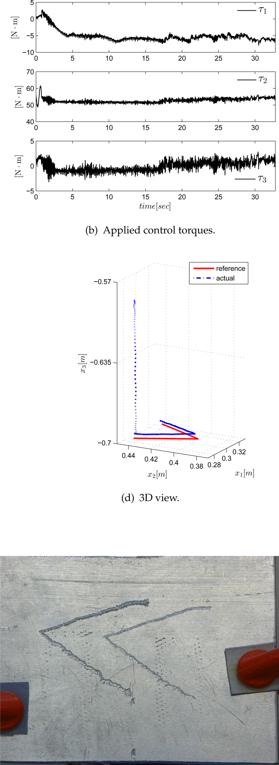
Traces over the surface

4. Conclusion

In this paper, a new family of stiffness control structures has been presented, designed to achieve the desired static behaviour of the interaction of a robot with the environment. The stiffness controller proposed by Salisbury can be considered as a particular member of the proposed family. The original idea of simulating a linear multidimensional spring with the end-effector of the robot manipulator - as the virtual spring's end - has been expanded to nonlinear models. The generalization consists of simulating a multidimensional spring - not necessarily linear - but with a well-defined mathematical structure. The new family of stiffness controllers is supported and validated with a rigorous stability analysis in the Lyapunov sense; it was found that the equilibrium point of the closed-loop system is locally and asymptotically stable in the Lyapunov sense.

In the absence of interaction forces, the controller becomes a position regulator in Cartesian space. Three case studies have been presented, including a new proposed controller. The case studies are as follows: the Cartesian PD controller (Salisbury's stiffness controller), the Cartesian tanh-tanh PD control structure, and the new controller which includes a proportional term of the Cartesian position error, and another term with the corresponding time-derivative; each term has a RQ form with their respective variable. Using the controllers, an engraving task was designed and performed in order to demonstrate the performance of all of the control schemes presented herein.

As a final comment, it is worth mentioning that the stability analysis was performed by using a Lyapunov criterion which exploits the properties reported for the model in Cartesian space. A final, more challenging experiment used to test the performance of the controllers consisted of a point-to-point application. In this case, the control structure was originally designed for regulation. Tackling the problem of tracking is proposed for future work, as well as dealing with the presence of parametric uncertainty in the robot model. In this case, an adaptive version of the control scheme might be a suitable solution approach [39]. In the tracking problem case, the analysis in Cartesian space represents a bigger challenge because not all the properties of the model in the joint space are mappable to the model in Cartesian space.

5. Acknowledgements

The first author would like to thank CONACyT and the ECOES programme for partially funding this work.

Footnotes

Appendix

Boundedness of the state equation solution

From the stability analysis, it was obtained that

\begin{matrix} V (\tilde{x}, \dot{x}) > 0 \\ \dot{V} (\tilde{x}, \dot{x}) < 0 \end{matrix}

which implies that $V (\tilde{x}, \dot{x})$ is a decreasing function in time [40] then,

(51)

0 < V (\tilde{x} (t), \dot{x} (t)) \leq V (\tilde{x} (0), \dot{x} (0)), \forall t \geq 0

Consequently, by considering the definition of $V (\tilde{x}, \dot{x})$ and the Rayleigh-Ritz theorem, the following is deduced,

(52)

\begin{array}{l} \frac{1}{2} λ_{m i n} {M_{χ} (t)} {‖ \dot{x} (t) ‖}^{2} \leq \frac{1}{2} {\dot{x}}^{T} M_{χ} (t) \dot{x} \\ \leq V (\tilde{x} (0), \dot{x} (0)) \end{array}

(53)

U_{a} (K_{p}, \tilde{x} (t)) - U_{a} (K_{p}, {\tilde{x}}_{E}) \leq V (\tilde{x} (0), \dot{x} (0))

where λ_min {M_χ} represents the minimum eigenvalue of the matrix M_χ.

Hence, the following maximum bounds are obtained,

(54)

\begin{array}{l} {‖ \dot{x} (t) ‖}^{2} \leq \frac{2}{λ_{m i n} {M_{χ} (t)}} [\frac{1}{2} {\dot{x}}^{T} (0) M_{χ} (0) \dot{x} (0) \\ + U_{a} (K_{p}, \tilde{x} (0)) + \frac{1}{2} {(x_{d} - x_{e} - \tilde{x} (0))}^{T} K_{e} (x_{d} - x_{e} - \tilde{x} (0)) \\ - U_{a} (K_{p}, {\tilde{x}}_{E}) - \frac{1}{2} {(x_{d} - x_{e} - {\tilde{x}}_{E})}^{T} K_{e} (x_{d} - x_{e} - {\tilde{x}}_{E})], \\ \forall t \geq 0 \end{array}

(55)

\begin{array}{l} U_{a} (K_{p}, \tilde{x} (t)) \leq \frac{1}{2} {\dot{x}}^{T} (0) M_{χ} (0) \dot{x} (0) + U_{a} (K_{p}, \dot{x} (0)) \\ + \frac{1}{2} {(x_{d} - x_{e} - \tilde{x} (0))}^{T} K_{e} (x_{d} - x_{e} - \tilde{x} (0)) \\ - \frac{1}{2} {(x_{d} - x_{e} - {\tilde{x}}_{E})}^{T} K_{e} (x_{d} - x_{e} - {\tilde{x}}_{E}), \forall t \geq 0 \end{array}

Additionally, consider the common structure $U_{a} (K_{p}, \tilde{x}) = h {(\tilde{x})}^{T} K_{p} h (\tilde{x})$ for the case studies included in this paper, then

(56)

λ_{m i n} {K_{p}} {‖ h (\tilde{x} (t)) ‖}^{2} \leq \underset{U_{a} (K_{p}, \tilde{x} (t))}{\underset{︸}{h {(\tilde{x} (t))}^{T} K_{p} h (\tilde{x} (t))}}

hence,

(57)

\begin{array}{l} {‖ h (\tilde{x} (t)) ‖}^{2} \leq \frac{1}{λ_{m i n} {K_{p}}} [\frac{1}{2} {\dot{x}}^{T} (0) M_{χ} (0) \dot{x} (0) \\ + U_{a} (K_{p}, \tilde{x} (0)) + \frac{1}{2} {(x_{d} - x_{e} - \tilde{x} (0))}^{T} K_{e} (x_{d} - x_{e} - \tilde{x} (0)) \\ - \frac{1}{2} {(x_{d} - x_{e} - {\tilde{x}}_{E})}^{T} K_{e} (x_{d} - x_{e} - {\tilde{x}}_{E})], \forall t \geq 0 \end{array}

The results (54), (55) and (57) imply that the state equation solution will be bounded for all initial conditions ${[\begin{matrix} \tilde{x} {(0)}^{T} & \dot{x} {(0)}^{T} \end{matrix}]}^{T}$ .

References

Siciliano

and Khatib

. Springer Handbook of Robotics. Springer, 2008.

Siciliano

and Villani

. Robot Force Control. Kluwer Academic Publishers, Norwell, MA, USA, 1st edition, 2000.

Caccavale

Natale

Siciliano

, and Villani

. Integration for the next generation: embedding force control into industrial robots. IEEE Robotics Automation Magazine, 12(3):53–64, 2005.

Hogan

. Impedance control - An approach to manipulation. I - Theory. II - Implementation. III - Applications. ASME Transactions Journal of Dynamic Systems and Measurement Control B, 107:1–24, mar 1985.

Volpe

and Khosla

. A theoretical and experimental investigation of explicit force control strategies for manipulators. IEEE Transactions on Automatic Control, 38(11):1634–1650, nov 1993.

Singh

S.K.

and Popa

D.O.

. An analysis of some fundamental problems in adaptive control of force and impedance behavior: theory and experiments. IEEE Transactions on Robotics and Automation, 11(6): 912–921, dec 1995.

Siciliano

Sciavicco

Villani

, and Oriolo

. Robotics: Modelling, Planning and Control. Springer Publishing Company, Incorporated, 2010.

Raibert

M. H.

and Craig

J. J.

. Hybrid Position/Force Control of Manipulators. Journal of Dynamic Systems, Measurement, and Control, 103(2):126–133, 1981.

Yoshikawa

Sugie

, and Tanaka

. Dynamic hybrid position/force control of robot manipulators-controller design and experiment. IEEE Journal of Robotics and Automation, 4(6):699–705, dec 1988.

10.

Lozano

and Brogliato

. Adaptive hybrid forceposition control for redundant manipulators. IEEE Transactions on Automatic Control, 37(10):1501–1505, oct 1992.

11.

Jeon

and Tomizuka

. Learning hybrid force and position control of robot manipulators. IEEE Transactions on Robotics and Automation, 9(4):423–431, aug 1993.

12.

Ferretti

Magnani

, and Rocco

. Toward the implementation of hybrid position/force control in industrial robots. IEEE Transactions on Robotics and Automation, 13(6):838–845, dec 1997.

13.

Gueaieb

Karray

, and Al-Sharhan

. A Robust Hybrid Intelligent Position/Force Control Scheme for Cooperative Manipulators. IEEE/ASME Transactions on Mechatronics, 12(2):109–125, 2007.

14.

Namvar

and Aghili

Farhad

. Adaptive Force-Motion Control of Coordinated Robots Interacting With Geometrically Unknown Environments. IEEE Transactions on Robotics, 21(4):678–694, 2005.

15.

Kumar

Panwar

Sukavanam

Sharma

, and Borm

. Neural network based hybrid force/position control for robot manipulators. International Journal of Precision Engineering and Manufacturing, 12(3):419–426, 2011.

16.

Chiaverini

and Sciavicco

. The parallel approach to force/position control of robotic manipulators. IEEE Transactions on Robotics and Automation, 9(4):361–373, aug 1993.

17.

Xia

Q. H.

Lim

S. Y.

Ang

M.H.

, and Lim

T. M.

. Parallel force and motion control using adaptive observer-controller. In SMC 2008. IEEE International Conference on Systems, Man and Cybernetics, pages 3143–3149, oct. 2008.

18.

Salisbury

J. K.

. Active stiffness control of a manipulator in cartesian coordinates. In 19th IEEE Conference on Decision and Control including the Symposium on Adaptive Processes, volume 19, pages 95–100, dec. 1980.

19.

Sang-Rok

Ho-Chan

Il-Hong

Bum-Jae

, and Chong-Won

. A compliance control strategy for robot manipulators using a self-controlled stiffness function. In 1995 IEEE/RSJ International Conference on Intelligent Robots and Systems 95. ‘Human Robot Interaction and Cooperative Robots’, volume 3, pages 179–184, aug 1995.

20.

Byoung-Ho

Nak-Young

Sang-Rok

Il-Hong

, and Young-Jo

. Intelligent compliance control for robot manipulators using adaptive stiffness characteristics. In ICRA 1999. IEEE International Conference on Robotics and Automation, volume 3, pages 2134–2139, 1999.

21.

Tischler

and Goldenberg

A.A.

. Stiffness control for geared manipulators. In ICRA 2001. IEEE International Conference on Robotics and Automation, volume 3, pages 3042–3046, 2001.

22.

Mehdi

and Boubaker

. Stiffness and Impedance Control Using Lyapunov Theory for Robot-Aided Rehabilitation. International Journal of Social Robotics, pages 1–13, 2011.

23.

Kazerooni

Sheridan

, and Houpt

. Robust compliant motion for manipulators, part I: The fundamental concepts of compliant motion. IEEE Journal of Robotics and Automation, 2(2):83–92, jun 1986.

24.

Seul

Hsia

T.C.

, and Bonitz

R.G.

. Force tracking impedance control of robot manipulators under unknown environment. IEEE Transactions on Control Systems Technology, 12(3):474–483, 2004.

25.

Sang-Hoon

Maolin

, and Pyung-Hun

. A Solution to the Accuracy/Robustness Dilemma in Impedance Control. IEEE/ASME Transactions on Mechatronics, 14(3):282–294, 2009.

26.

Mehdi

and Boubaker

. Impedance Controller Tuned by Particle Swarm Optimization for Robotic Arms. International Journal of Advanced Robotic Systems, 8, 2011. DOI: 10.5772/45692.

27.

Mendoza-Gutiérrez

Reyes

Bonilla-Gutiérrez

, and González-Galván

E.J.

. Proportionalderivative impedance control of robot manipulators for interaction tasks. Proceedings of the Institution of Mechanical Engineers, Part I: Journal of Systems and Control Engineering, 225(3):315–329, 2011.

28.

Bonilla-Gutiérrez

Reyes

Mendoza-Gutiérrez

, and González-Galván

E. J.

. A Dynamic-compensation Approach to Impedance Control of Robot Manipulators. Journal of Intelligent & Robotic Systems, 63:51–73, 2011.

29.

Chenguang

Ganesh

Haddadin

Parusel

Albu-Schaeffer

, and Burdet

. Human-Like Adaptation of Force and Impedance in Stable and Unstable Interactions. IEEE Transactions on Robotics, 27(5):918–930, 2011.

30.

Anderson

R.J.

and Spong

M.W.

. Hybrid impedance control of robotic manipulators. IEEE Journal of Robotics and Automation, 4(5):549–556, oct 1988.

31.

Carelli

and Kelly

. An adaptive impedance/force controller for robot manipulators. IEEE Transactions on Automatic Control, 36(8):967–971, aug 1991.

32.

Hosseinzadeh

Aghabalaie

Talebi

H.A.

, and Shafie

. Adaptive Hybrid Impedance Control of robotic manipulators. In IECON 2010 – 36th Annual Conference on IEEE Industrial Electronics Society, pages 1442–1446, nov. 2010.

33.

Kurfess

T. R.

. Robotics and Automation Handbook. Taylor & Francis, 2005.

34.

Takegaki

and Arimoto

. A New Feedback Method for Dynamic Control of Manipulators. Journal of Dynamic Systems, Measurement, and Control, 103(2):119–125, 1981.

35.

Canudas-de Wit

Bastin

, and Siciliano

, editors. Theory of Robot Control. Springer-Verlag New York, Inc., Secaucus, NJ, USA, 1st edition, 1996.

36.

Siciliano

Robot control. In Samad

Tariq

, editor, Perspectives in control engineering: technologies, applications, and new directions, pages 442–461. Wiley-IEEE Press, 2000.

37.

Vidyasagar

. Nonlinear Systems Analysis. Prentice Hall, 1993.

38.

Chávez-Olivares

C. A.

Reyes-Cortés

González-Galván

E. J.

Mendoza-Gutiérrez

, and Bonilla-Gutiérrez

. Experimental Evaluation of Parameter Identification Schemes on an Anthropomorphic Direct Drive Robot. International Journal of Advanced Robotic Systems, 9, 2012. DOI: 10.5772/52190.

39.

Wang

and Yongchun

. Adaptive inverse dynamics control of robots with uncertain kinematics and dynamics. Automatica, 45(9):2114–2119, 2009.

40.

Khalil

H.K.

. Nonlinear Systems. Prentice Hall, New Jersey, 2002.

On Stiffness Regulators with Dissipative Injection for Robot Manipulators

Abstract

Keywords

1. Introduction

2. A new family of stiffness regulators and dissipative injection

2.1 A dynamic model of robot manipulators

2.4.1 PD-type controller structure

5. Acknowledgements

Footnotes

Appendix

References