
Abstract
To date, running robots are still outperformed by animals, but their dynamic behaviour can be described by the same model. This coincidence means that biomechanical studies can reveal much about the adaptability and energy efficiency of walking mechanisms. In particular, animals adjust their leg stiffness to negotiate terrains with different stiffnesses to keep the total leg-ground stiffness constant. In this work, we aim to provide one method to identify ground-robot impedance so that control can be applied to emulate the aforementioned animal behaviour. Experimental results of the method are presented, showing well-differentiated estimations on four different types of terrain. Additionally, an analysis of the convergence time is presented and compared with the contact time of humans while running, indicating that the method is suitable for use at high speeds.
1. Introduction
Although there are only a few agile legged machines, research into faster robots is increasing [2, 20, 22, 26, 38, 39, 42]. Nevertheless, these robots are still outperformed by animals. Thus, there remains a lot to learn from their biological counterparts, particularly in the case of adaptability and endurance.
It is generally accepted that a spring-loaded inverted pendulum (SLIP), i.e., a point mass on a simple Hookean spring models the basic dynamics of running remarkably well. This model explains the mechanics of running of several animals, including humans [1, 8, 9, 11, 14, 17, 35]. Moreover, it has been applied to describe the dynamic behaviour of running robots [2, 19, 41]. This coincidence implies that the conclusions obtained from studies of animal-running dynamics should also be applicable to robots.
The stiffness of the leg spring (the spring used to model the energetics of running) is an important parameter in the dynamics of running because it influences contact time and stride frequency [15, 36]. Biomechanical studies of running reveal that animals, including humans, can adjust the stiffness of their leg spring. Experimental data show that this adjustment depends on velocity [3], stride frequency [15] and surface stiffness [16, 28, 37].
Changes of stiffness to increase velocity are small, and the same effect can be achieved by increasing the leg stride (angle swept by the leg) while maintaining the same stride frequency [14]. Moreover, stiffness changes depending on stride frequency are made to preserve a certain velocity [15]. In contrast, stiffness changes made to accommodate different surface stiffnesses have more important consequences. First, if the same leg stiffness is used on every surface, the body can be put out of balance whenever an abrupt change in the surface stiffness occurs; however, adjusting the stiffness offers a smooth transition between surfaces [17]. Second, adjusting the leg stiffness to accommodate different terrains can lead to more efficient running because increasing the leg stiffness as the terrain stiffness decreases leads to less mechanical work being done by the leg and more mechanical work being done by the terrain [18]. In other words, by adjusting the leg stiffness to accommodate terrain adaptability, energy efficiency can be enhanced.
To extrapolate this conclusion to legged robots, one important consideration is how to know when the stiffness adjustment must be performed. Animals, or at least birds [12] and humans [17], change their leg stiffness before stepping onto a new surface when they are knowingly changing surfaces. Nonetheless, the question remains as to how they adjust leg stiffness one the first occasion, when the surface is unknown. This question leads to the idea that some sort of information about ground stiffness must be acquired directly from the surface (on at least) the first time they step on it while running.
The aim of this study is to provide a method to obtain ground stiffness information with a legged robot rather than to propose methods to adjust leg stiffness, although much research effort is being put into solving the latter problem [5, 7, 24, 25, 27]. Nevertheless, this application is kept in mind throughout the paper. The reason for this approach is that identifying the leg-ground stiffness while running must be treated as an independent problem due to the various application restrictions (these restrictions will be clarified in the next section). Additionally, the ultimate goal of our identification method is not to estimate the ground stiffness as accurately as possible but rather to estimate the robot-ground interaction properties, which are the control target.
Another important reason for this study is that, in real-world conditions, it is not possible to predict every contact surface that will be encountered. Nevertheless, it might be possible to store the information of ground stiffness beforehand in order to adjust the robot's leg stiffness using some type of perception, although perception (e.g., vision) has its limits in detecting different surfaces; for example, two different terrains might be hidden under a given cover. For this reason, in order to obtain information about the terrain, we propose to use an event-driven system identification method. This method is based on the well-known recursive least squares (RLS) method [23, 33] and aims to estimate the parameters of the ground as modelled as a spring dashpot. The RLS method was chosen because it is computationally efficient, allowing online computation, and because it has shown good convergence and accurate results in similar applications.
This paper is organized as follows. Section 2 presents the contact model we used as well as a brief summary of the detail, and the necessary considerations for its application are established. Section 4 describes the experimental setup and the implementation of the algorithm on a leg prototype. In Section 5, the experimental results are presented, and finally, the conclusions are provided in Section 6.
2. Background
Most of the biomechanics research on the adaptability of humans and other animals to different terrains has focused on leg stiffness [3, 12, 14-17, 28, 35-37]. However, there are studies that show that the centre of mass (COM) of humans running on dissipative materials (such as sand) follows a bouncing motion with the same stride frequency as on hard surfaces [31, 43]. For this reason, to incorporate an estimate of the energy dissipation, the contact model chosen in this work was the spring dashpot model [7, 21]:

where Fc is the contact force, δ is the displacement of the ground, and k and b are the stiffness and damping constants of the surface, respectively. This particular model was also chosen because it is linear and thus relatively easy and quick to identify. Other more complex models that describe the contact dynamics more accurately are nonlinear and require special techniques of system identification, more execution time, and frequency-richer data than the data that can be obtained using a legged robot (while walking or running). The relatively poor frequency information of the data obtained using a legged robot is because the types of signals that can be given to excite the ground mechanical system using a legged robot are limited; other specialized signals that allow for the extraction of frequency-rich information can cause the robot to lose balance, which is undesirable.
As stated above, the identification procedure was developed based on the well-known RLS method for system identification. This choice is justified by the fact that it offers a low modelling error (defined in the next section) when used in similar applications, e.g., identifying the contact properties of a determined surface [4]. Here, a brief summary of the RLS method is provided for the sake of completeness. However, the interested reader is referred to the specialized literature [10, 23, 33].
2.1 RLS method
The RLS method consists of applying the least squares criteria to minimize the modelling error of a process expressed as a linear regression, and it can be summarized as follows:
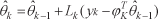

were
It is important to note that this algorithm can cause matrix P to become negative because of round-off errors; to avoid this situation, we have used Bierman's U-D factorization algorithm [32] to compute matrix P and update matrix L.
Note that Equation (1) is a linear differential equation, not an autoregressive process. Nonetheless, it can be transformed into a linear regression by simply rewriting the equation as follows:

where:


Thus, the modelling error is defined as:

It is important to note that Equation (1) can be written in different forms. To clarify the choice of Equation (7), let verr denote the unknown modelling errors and the noise in the measurements of the regression (i.e., force, velocity and position). As such, we can write the estimations as:


Now, if we apply a least squares estimation to the above equations, this yields [33]:

where M(φi) is a matrix that depends on the regressor and w is a vector containing the modelling errors and the noise in the measurements. These last equations can be used to find and upper bound in terms of the largest singular value of the matrix M(φi). Let us denote this singular value as σmax (Mφi)). Thus, we can write the upper bound as:


The previous analysis suggests that if the maximum singular values are equal, then equation (??) provides the best estimate. Moreover, the results of a comparison between the results applied to the data will be provided further below.
Now, using the linear regression form of Equation (1), it is possible to apply the RLS method directly to the identification problem. However, because our intention is to use the algorithm in a legged robot (namely, to identify the contact properties of the ground using legs), a few concerns arise: When should the identification start? How are the samples taken? Is it necessary or even practical to use the system identification during the whole gait cycle? The next section is devoted to answering these questions and it describes in detail the system identification procedure proposed in this work.
3. Identification procedure
Before describing the identification procedure, it is useful to review the literature concerning haptic interfaces. In that field, several studies have focused on recognizing the dynamic properties of manipulated objects [13, 29, 30, 34], These studies have mainly used two approaches: active sensing methods [34], which offer precise and accurate estimations of the properties in the presence of noise, but which require specialized control techniques; and passive sensing methods [13, 29, 30], in which the identification procedure is independent of control but which are less efficient [29].
3.1 Basic considerations
Although the application addressed in this paper is different and some necessary considerations may differ, some of the conclusions of the previous work on haptic interfaces still apply. Active sensing, although more precise, is not suitable for use in legged robots because using a specialized control method for the identification would disrupt the robot running behaviour, which might cause destabilization. Moreover, active sensing methods continuously preform the system identification. On the other hand, the system identification literature establishes that identifying a system in equilibrium is useless because information about its dynamic behavior cannot be obtained. This implies that the identification should start as soon as the foot touches the ground and cease when the foot leaves the ground or the contact has been stabilized Therefore, passive sensing is the logical choice.
Considering this last remark, one possible state diagram of the identification procedure can be envisaged (see Figure 1).
This state machine consists of two basic states: (a) the “idle” state, in which all of the matrices and vectors of the identification method are reset to their original values and wait until the leg contacts the ground (in this case, it goes to the next state); and (b) the “identify ground impedance” state, which performs the system identification according to the RTS method described in the previous section.
Note that the “idle” state is said to reset the system identification algorithm. This feature is not strictly necessary if the robot steps on the same surface more than once. In fact, using the estimates of a prior identification with a given surface might enhance the accuracy of the estimation. Nevertheless, we chose to reset the algorithm here in order to prepare the robot for a new surface, as using the estimates of another surface as the starting point might affect convergence.
At this point, it is important to discuss the sampling frequency. When controlling a system, the sampling frequency should be as high as possible so as to maintain good tracking error for the reference trajectories, regardless of the control method used. Nevertheless, in this case the control loop frequency (2,000 kHz) may be too high and produce a quantization error in the identification algorithm. These errors might lead the system identification algorithm to fail because it might consider the system to be in equilibrium. Thus, the sampling frequency should be chosen accordingly in order to reflect the changes in the system response. A more detailed discussion of the sampling frequency will be addressed in Section 5.
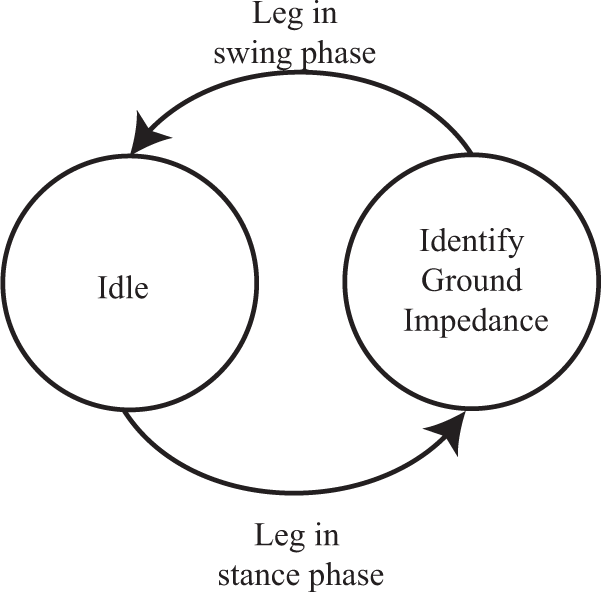
State diagram of the system identification method
3.2 Robot structure considerations
Another important point is the effect of the robot's structure on the identification. Let us consider a robot during a bouncing gait in contact with the ground. The behaviour of the robot should resemble a SLIP. Nevertheless, many robots have rigid links, and the spring compression at the lowest part of the stance phase could be achieved by flexing a rigid leg. In this case, there is no need to consider deformation on the robot's links, and the state diagram described in the above section might be sufficient.
In contrast, the robot might not be constructed entirely of rigid links, as is the case with many robots designed to run [20, 22, 26, 38-40, 42]. In this case, when computing the ground penetration (δ), the compression of the robot's links must be considered to obtain an accurate measure.
With this last consideration, a modified version of the block diagram in Figure 1 with a wider range of applicability can be designed (see Figure 2). In this diagram, two new states have been included, an “initialization” state and a “compute COM position” state. The initialization state computes the initial leg position, its maximum length and the COM position when the algorithm starts. Next, the “compute COM position” state is included to compute the COM's vertical displacement to pass the information to the next identification state at the beginning of the stance phase. Following this, the “identify ground impedance” state can compute the COM's vertical displacement from the moment at which the foot makes contact with the ground. Thus, the ground penetration will be equal to the difference between the COM's displacement and the leg's compression.

State diagram of the system identification method considering the robot structure
Note that to increase the adaptability to the terrain, the ultimate goal of the identification is not to estimate the ground properties as accurately as possible but rather to estimate the robot-ground interaction properties. Thus, the leg stiffness can be adjusted to hold the total robot-ground impedance constant, which is desirable because biomechanical studies in humans [17, 18] show that humans adjust their leg stiffness to maintain the total impedance as constant, leading to more energy-efficient running.
In the next section, the system identification procedure is implemented on a robotic leg prototype [5, 20] and used to identify the impedance of the leg in contact with different types of ground.
4. Experimental setup
The HADE leg prototype (see Figure 3) is a planar, three-degree-of-freedom (DOF), under-actuated mechanism featuring the characteristics of a horse leg [20]. It is actuated by two series elastic actuators (SEAs), one at the hip and one at the knee, while the ankle joint is passively driven by an extension spring with a stiffness constant Ks = 3, 113 N/m. The hip and knee actuators have a spring with an encoder attached that acts as a force sensor with a resolution of 1.2 N per count and an encoder for measuring the position with a resolution of 50.8e-6 m per count. The ankle has a linear encoder with a resolution of 224e-6 m per count, which is equivalent as 0.69 N per count.
The leg is fixed to the wall by a sliding rail, so horizontal movements of its COM are restricted but it is capable of moving vertically. Moreover, the vertical movement is limited by a mechanical top at the bottom in order to prevent falling when the leg is not in contact with the ground. Incremental encoders are used to measure the position of each joint and to indirectly measure the joint torque by measuring the spring deflection at each actuator and the fetlock spring. The leg implements a position control scheme based on inverse kinematics and proportional-integral-derivative (PID) controllers at each active joint (hip and knee), while ground contact is detected by monitoring the ankle spring torque. The control was implemented using a National Instruments PXI-1024Q (Austin, TX, USA) and had an execution time of 0.5 ms per cycle, while the identification algorithm had an execution time of 5 ms per cycle.
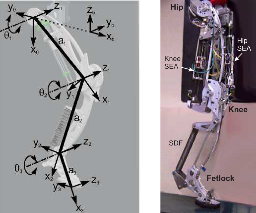
The HADE Leg Prototype. Conceptual design (left). Real prototype (right).
The complete experimental setup is shown in Figure 4. The foot was placed over two different surfaces and then commanded to move upwards until it was not in contact with the surface. Next, it was commanded to stay in that position for 0.5 s. Afterwards, it was commanded to return to its initial position (in contact with the ground) and stay there for another 0.5 s. This procedure was repeated twice for each experiment.

Experimental setup. Leg stepping over the variable-impedance box (right) and sand (left).
Moreover, the experiments were performed on four different types of terrain: (A) rigid ground; (B) an adjustable-impedance metal box [4], designed to resemble the behaviour of the spring dashpot contact model (see Equation (1)); (C) river sand; and (D) rocks. The last two types of terrain were used by filling a wooden box with the corresponding material (see Figure 4).
4.1 Implementing the system identification algorithm on the HADE leg
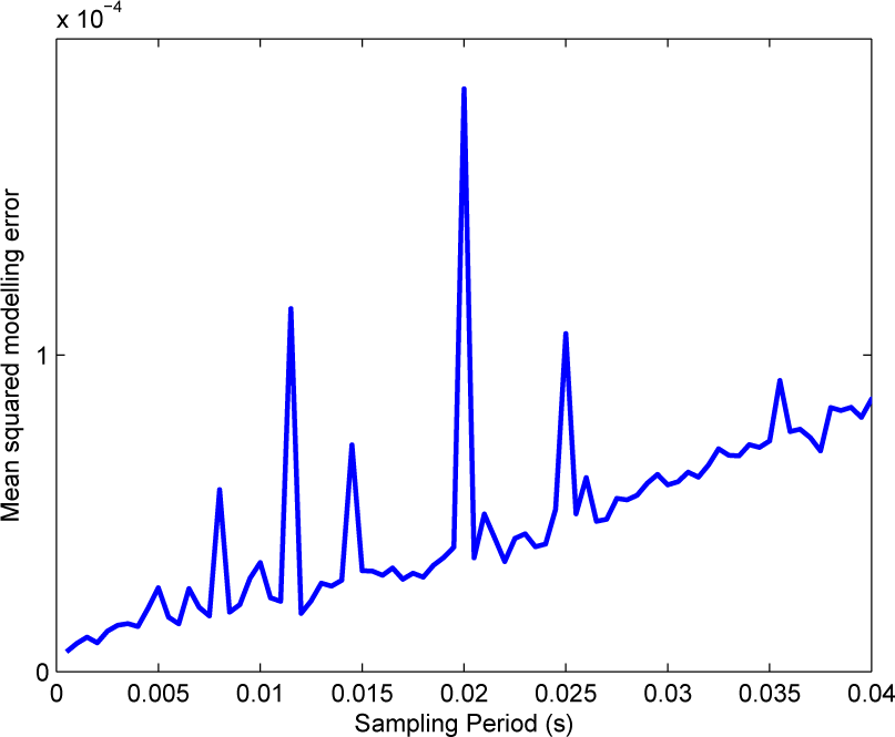
Prior to the implementation on the HADE leg, experiments were performed on data obtained using the experimental setup published in [4] with the RLS algorithm to choose values for the forgetting factor λ and the sampling frequency. Fig. 5 and 6 show the mean square modelling error against the sampling time for the metal box and the river sand, respectively. The data used in these simulations were collected by applying a force square wave to the metal box and the river sand; the force wave consisted on a 60 N force for 15 seconds; next, a square wave of ± 10 N around the 60 N force offset for 10 s; afterwards, the square wave amplitude was increased to 40 N for 10 s; at this time, the frequency was changed to 1.5 Hz for 10 s more; and finally, the reference force was set to 0 for the last 10 s of the experiment [4]. The results in Fig. 5 and 6 by resampling the data using frequencies between 2 kHz and 25 Hz and applying the RLS algorithm to 10 repetitions of the experiment for each type of terrain.

Mean square error vs sampling time for the metal box
In Fig. 5, it is shown that – generally – as the sampling frequency decreases (i.e., the sampling time increases), the modelling error increase (except for the sampling frequencies between 2 kHz and 333.3 Hz, where the error decreases). This is explained by the quantization error introduced by the position encoders' measuring position. Nevertheless, when the algorithm was applied to the river sand, the modelling error always increased as the sampling frequency was reduced. The difference is because the river sand is less stiff, and thus there are larger variations in the position for the same force; therefore, the quantization error has less influence on the result. Nonetheless, in Fig. 6 and 8, the errors are one order of magnitude larger than the errors shown in Figs. 5 and 7. This has a twofold explanation: the first reason for why this occurs is that the errors shown here are not normalized, and thus the errors with the river sand are larger because it is less stiff and there are larger variations in position; the second and most important reason is that, in the case of the river sand, the model is less accurate as this type of terrain presents nonlinear behaviour, and the identified model is a linear approximation of the system.
Mean square error vs sampling time for river sand
As the algorithm is intended to be used with different types of terrain, we have chosen a sampling frequency of 200 Hz, partly because it presented a near-minimum modelling error when used in a terrain that resembles our model. Moreover, when the algorithm was implemented with the PXI-1024Q, higher sampling frequencies interfered with the execution of the control loop. The problems explained here could be solved by using a computer with more computational power and with the use of higher resolution encoders.
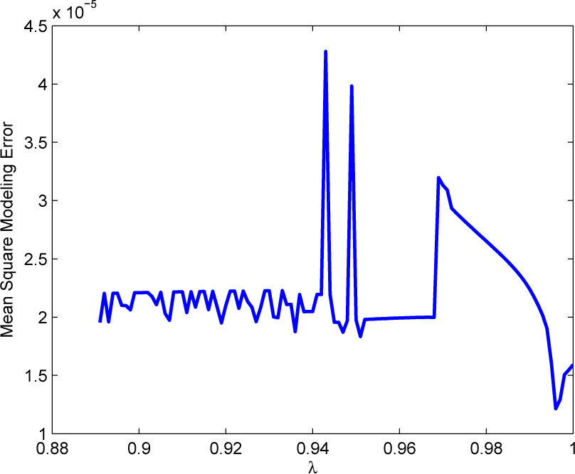
To choose the forgetting factor, the algorithm was applied to the same data as the sampling frequency experiment, using values of λ between 0.89 and 1. Figs. 7 and 8 show the mean square modelling error vs. λ for the metal box and the river sand, respectively.

Mean square error vs λ for the metal box
In Fig. 7, it can be seen that values of λ between 0.89 and 0.94 lead to a more or less constant modelling error; nevertheless, as lambda increases from 0.94 to 0.99, the modelling error decreases until it reaches its minimum around λ = 0.98 and then increases a little between λ =0.99 to λ = 1. In Fig. 8, a similar behaviour is observed, although the constant behaviour of the modelling error is from λ = 0.89 through λ = 0.97; then the error increases sharply and starts decreasing until it reaches its minimum at λ = 0.996 and increasing towards λ = 1.
Mean square error vs. λ for the river sand
Considering the results of the previous experiments, we have chosen a value of λ of 0.996, as it presented an error value near the minimum with the metal box and the minimum error value with the river-sand.
Once the values for lambda and the sampling frequency were chosen, we tested the algorithm with the same data for different forms of Equation (1). The results of this implementation are shown in table 1, in which the errors have been divided by the squared sum of the measured output for meaningful comparison. That is:

where e is the normalized error, Ei are the residuals and Yi is the measured output of the system. As can be seen from the table, the chosen form of the recursion performs better that its counterparts, as suggested by equations (15) through (17). A detailed analysis of the residuals of the RTS method with different types of terrain can be found in [4], where it is shown that the residuals exhibit evidence of unmodelled behaviour in both nonlinear and linear terrains due to quantization errors and non-linearities in the robot.
Mean square error for different forms of Equation (1)

Once the parameters of the identification algorithm were chosen, to implement the system identification on the HADE leg, given the leg characteristics, it was necessary to use the state machine depicted in Figure 2. Here, during the “initialization” state, both the total extended length of the ankle spring and the offset force had to be computed to obtain an accurate measure. The latter is a consequence of the incremental encoders mounted on the leg and the fact that the spring starts pre-compressed because of the leg's weight. This implementation has also been presented in [6].
To compute the ground penetration, and because there was no accelerometer or inertial measurement unit (IMU) mounted on the leg, we used the COM as the origin of the coordinate frame. Thus, making ZCOM = 0 made it necessary to consider the ground penetration as the difference between the foot's vertical position Zfoot and the ankle's vertical position Zankle. Moreover, it is important to note that in the implementation, we not only measure the ground penetration but also the compression in the leg due to its weight. This is because we only have access to the displacement of the contact interface between the robot and the ground. Therefore, in the algorithm we are performing the identification on the combined robot-ground system, which for consistency with the rest of the paper we call ‘ground penetration’ δ. Nevertheless the reader should be aware that hereafter, when we say ‘ground penetration’, we will be referring to the combined displacement of the leg and the ground (δ = δground +δrobot), which is equal to the difference between Zfoot –ZAnkle (see Figure 9).

Identification parameters
As can be seen in Fig. 9, δr obot can vary only due to flexion of the foot, even without observable ground penetration.
Nevertheless, as our primary objective is to identify the total impedance of the ground-robot system, this is not an issue. In other words, if the ground is perfectly rigid (or else stiff enough), the algorithm will identify the leg's impedance, which is a logical result since the total stiffness will converge to the leg's stiffness. This is because, when computing the equivalent stiffness of a series of springs:

The exerted foot force was computed using the force measurements on the ankle spring only. This force was a good approximation because the torque transmitted by the spring to the ankle was the same as the torque transmitted by the ankle to the ground, as they were connected to each other through a rigid link. Nevertheless, the arm from the spring to the ankle was variable; therefore, this arm had to be computed for each force measurement. Technically, the arm from the foot to the ankle was also variable, as it depended upon the area of contact of the foot; however, this variation was small because the foot touched the ground at approximately the same contact point every time.
One last thing to note about the implementation of the identification algorithm on the HADE leg is the detection of contact. As the HADE leg has no force or contact sensor at the sole of the foot, it was necessary to monitor the ankle spring. If the spring is sufficiently rigid such that it does not oscillate when the leg is in the swing phase, it suffices to monitor only the spring and launch the identification algorithm when its value is below zero (the force of the spring has the opposite sign from the contact force because of the manner in which it is attached to the leg). This is the case for the HADE leg, and so contact is detected whenever the value of the force becomes negative.
Nevertheless, note that if the spring does oscillate, then the contact can be detected when the force reaches a certain threshold. The value of the threshold will depend upon the oscillation, and it can also be computed in the “compute COM position” state.

Scaled Gaussian bell of the estimation results for the stiffness (left) and damping (right) coefficients for the metal box (continuous line) and the rigid ground (dashed line)
In our case, the threshold was computed when the leg left the ground. This is because the encoders used were incremental and the leg started resting on the ground. This caused an offset in the force measurements when the leg was lifted.
5. Results
The results of the identification performed on the rigid ground and variable-impedance box are presented in Figure 10, which consists of the scaled Gaussian bell of the estimated total stiffness (left) with the box (continuous line) and rigid ground (dashed line), as well as the Gaussian bell of the damping coefficient (right) for the box (continuous line) and rigid ground (dashed line). The scaling was performed as follows:

where f is the Gaussian function obtained from the data, n is the distribution of the values of the histogram of the data, and G is the Gaussian bell to be plotted.
Scaled Gaussian bells were chosen to offer an intuitive representation of the results. Though they do not offer a quantitative result, the figure shows that the majority of the estimated values lay at approximately 2,750 N/m and 3,500 N/m for the box and rigid ground, respectively.
Moreover, from the curves it can be seen that the results for both types of ground are differentiated, as the majority of the curves' areas do not overlap with each other. In addition, and in order to offer a quantitative evaluation, Table 2 shows the mean value, the standard deviation of the estimated values, the theoretically calculated value, and the mean of the estimation error.
Note that in the case of the rigid ground, the identified stiffness corresponds to the leg's stiffness, as the series combination of two series springs when K1 » K2 tends to K2. Moreover, in the experiment, the final position of the leg on the ground was the extended position, which meant that the leg's stiffness was approximately equal to the ankle spring because the series elastic actuator's elastic constant was 15 times higher than that of the ankle spring.
Estimation results for the stiffness of the box and rigid ground

The theoretical values given in Table 2 were computed with the stiffness values supplied by the manufacturer, so the tolerance error was also included in the identification. The damping constant was not included in the table because this value was unknown for both the leg and the box, and no theoretical value could be used to evaluate the performance of the identification method. However, the estimated values of the damping coefficient and their standard deviation are shown in Table 3.
Figure 11 shows the results of the identification of the sand and rocks. The figure shows the scaled Gaussian bells of the estimated values of the stiffness (left) and damping coefficients (right) for the rocks (dashed line) and the sand (continuous line). In the curves, it can be observed that the two types of ground have well-differentiated stiffnesses. In the case of the rocks, the majority of the points were concentrated at approximately 2,500 N/m, while in the case of the sand they were concentrated at approximately 1,100 N/m. Note that both of these terrains generate nonlinear behaviour, such as elastic deformation (they can be compressed due to the geometrical rearrangement of the rocks or the grains of sand). Thus, the dispersion standard deviation of the estimation should be larger than in the previous case.
Estimation results for the damping coefficient of the box and rigid ground


Scaled Gaussian bell of the estimation results for the stiffness (left) and damping (right) coefficients for the rocks (continuous line) and the river-sand (dashed line)
Regarding the damping coefficients, it can be inferred from the curves that the damping coefficients of both types of terrain were relatively close. In the case of the rocks, most of the estimated values were approximately 200 Ns/m (see Figure 11 right), while in the case of the sand the values were concentrated at approximately 600 Ns/m. To provide quantitative results, the mean and standard deviation of the estimated values for the rocks and sand are presented in Table 4.
Estimation results for the sand and rocks

Table 4. demonstrates that the standard deviation of all the quantities was high compared to their respective mean values. This result indicates unmodelled behaviour, which was to be expected because the model used in this work was linear, whereas the terrain behaviour is not. Nonetheless, they had well-differentiated values of stiffness. Expressed mathematically:

where K indicates the mean value of the samples and std(K) indicates the standard deviation. In contrast, the damping coefficients did not appear useful in discriminating between the terrains. Nevertheless, these coefficients did indicate the energy losses during locomotion, so they can be used to compensate for that energy.
The value of the standard deviation for the rigid ground and adjustable-impedance box was approximately 2% of the mean, while the values for the rocks and sand were between 23% and 30%. The standard deviation was relatively high in both cases because there was unmodelled behaviour due to motor transmissions, joint friction and other factors that are intrinsic to the leg system. Therefore, the implemented parameter estimation method provides more accurate results for the rigid ground and the adjustable impedance box, as these environments are reasonably well modelled by Equation (1).
5.1 Convergence time
Another important aspect of identifying the terrain contact properties with a legged robot is the convergence time. This parameter is important because the identification should be performed completely within the stance phase of any particular leg.
Figure 12 shows the average values of the components of the vector of parameters used in the identification of sand versus time. Note that the figure shows the values of θ = [1/k, b/k], which was intentional because the vector of the parameters was initialized with θ1 = 1/k = 0, implying that k → inf (which might have been confusing for representation purposes).

Estimated values of the parameters 1/k (dashed line) and b/k (solid line) obtained by applying the identification algorithm to sand versus time
The parameters 1/k and b/k reach convergence at approximately t = 0.3s. In contrast, biomechanical studies show that the contact time of humans when running on rigid and soft elastic surfaces at a speed of 3.7 m/s is approximately 0.2 s [28]. McMahon, in [37], reported that the contact time for a human running over pillows at a speed of 4 m/s was over 0.3 s. Although it is true that contact time decreases with increasing speed, these results show that the algorithm can be used for running at moderate speeds (on viscous terrains). Moreover, it is important to note that the average velocity of legged robots is below 2 m/s (with the exception of Boston Dynamics' Cheetah).
Moreover, the convergence time differed as the impedance varied (i.e., with different systems). Figure 13 shows the values of the estimated parameters with the rigid ground. The convergence time was approximately 0.15 s, which was lower than the value measured by Kerdok et al. [28]. This value varies with speed, so the proposed algorithm can be used at relatively high speeds as long as the contact time is higher than 0.15 s.

Estimated values of the parameters 1/k (dashed line) and b/k (solid line) obtained by applying the identification algorithm to rigid ground vs time
The above discussion is valid with an ankle spring with Kspring = 3, 113 N/m and with the execution time of 5 ms. If the sampling frequency is increased, then the convergence time can be reduced. However, as was stated in previous sections, this would require encoders with a higher resolution.
6. Conclusion
According to biomechanical studies, humans and animals adjust their leg stiffness to maintain the same mechanics when running on surfaces with different stiffnesses. This adjustment allows them to achieve higher energy efficiency on more flexible terrains while maintaining balance. This behaviour can also be beneficial for robots, as their behaviour during running can be explained by the same mathematical model as animals. Following this idea, we have described in detail a system-identification procedure based on the RTS method to be used in legged robots. The algorithm identifies the combined impedance of the leg and the ground simultaneously. Moreover, it considers several aspects, such as ground modelling, the structure of the robot and the sampling frequency.
Additionally, we experimentally evaluated the HADE leg (an under-actuated 3-DOF planar mechanism). The results of the evaluation are encouraging, as the algorithm offers good convergence and tracking when applied to elastic terrains (a rigid ground and adjustable impedance box) in addition to unknown dissipative terrains (sand and rocks). Despite the nonlinearity of the behaviour of these last two terrains, the algorithm is capable of producing well-differentiated estimations of their respective stiffnesses and produces an estimation of their damping properties.
Moreover, the convergence time of the algorithm was analysed, comparing the convergence time with the published data on contact time in running humans. This comparison shows that the algorithm is faster than the contact time of human running (3.7 m/s). Thus, it can be used at relatively high velocities if the contact time is lower than 0.15 s.
One major disadvantage of our approach is that if the walking speed is high, the information can only be used in the next step. Thus, in the worst case scenario (where the impedance of the ground varies substantially between one step and another) this makes the model-based approach a better option. Nevertheless, model-based approaches requires a model of the robot, while our approach does not. Moreover, this method can be used to construct a map of such types of terrain to be used later for other robots to adjust their impedance. Another possible solution is to use a combined approach, using the proposed method to compute the impedance of the ground on the fly and combine it with a model-based approach to adjust the desired impedance as the preliminary parameters of the contact model are updated.
Footnotes
7. Acknowledgements
This work was partially funded by the Spanish National Plan for Research, Development and Innovation through grant DPI2013–40504-R. Mr. Juan Carlos Arevalo and Mr. Manuel Cestari would like to thank the Spanish National Research Council and the Spanish Ministry of Economy and Competitiveness for funding their PhD research.