
Abstract
Modern production systems must guarantee high performance. Increasingly challenging international competition, budget reductions for the health sector and constant technological evolution are just three of the many aspects that drive pharmaceutical companies to continuously improve the productivity of their lines.
The scientific literature has for many years been proposing calculation models for estimating the productivity of a machine. One of the most famous, and still used, is overall equipment effectiveness (OEE). This allows the calculation the valuable output considering the six ‘big losses’. The limitations of this approach are noticeable when considering a production line instead of a single machine. Numerous researchers have proposed alternative methods or changes in OEE, to be able to cover the widest spectrum of possible cases.
In this study, we wanted to evaluate how such theoretical models related to OEE are actually able to represent the world of tight production flows or whether, in these cases, a more complex type of simulation should be preferred. To do this, we carried out a case study of a production line in the pharmaceutical industry, and the results showed that the simulation approach gives better results because of the peculiarities not considered by the theoretical models.
1. Introduction
In the industrial sector it is increasingly common to employ methods and tools to measure production performance. There are various reasons why, in recent years, there has been a steady increase in the adoption of these techniques. The main reason is the need to quantify the achievement of the objectives set by the companies and, consequently, to identify areas of improvement [1].
In the literature there are many papers that deal with the measurement of system performance [2] [3] [4] [5]. They emphasize their historical evolution over the years and the ways in which they had to adapt to the changing features of the target market; first of all, globalization. In the production field in particular this shifted the focus of performance from the financial to different aspects, widely spread until at least the end of the 1980s [6]. Since productivity is so crucial in production management, many methods have been developed recently in order to improve the performance of a line in various industrial fields [7].
The performance measures used in production management, focus on quick inefficiency identification. In particular, it is essential to measure actual performance and compare it to the theoretical one, in order to identify which elements make it less effective than its hypothetical potential.
As a production process is generally composed of several machines that contribute to the production of the product coming out of the same process, performance measurement is primarily concerned with individual machines. Throughput rate and capacity utilization are widely used for this purpose [8]. For low production rates, such indicators are less effective and more structural approaches are preferred [9]. However, throughput and capacity utilization provide a general measure of the operation of a machine, without giving information about the causes of inefficiencies or any guidance on how to resolve them. For this reason the need was felt to define an index that would enclose the main characteristic features of a production system.
In 1998, Nakajima [10] introduced the concept of overall equipment effectiveness (OEE), a key element for the implementation of total productive maintenance (TPM). Based on this concept, the semiconductor equipment and materials international (SEMI), defined an index to measure the efficiency of equipment. The OEE indicator provides a measure of the actual productivity of a machine with respect to the theoretical one. The causes of this difference are associated with the so-called six big losses, which are usually defined in terms of three parameters: availability (A), performance (Ep) and quality (Q).
The availability parameter (see Figure 1) refers to the loss of productivity due to breakdowns and setups, performance efficiency takes into account the minor and non-measurable stops, while the quality index considers scraps and reworks. These productivity losses mean that the OEE parameter is less than one, as actual production will never be equal to theoretical production.

Outline of OEE calculation according to Nakajima. Subtracting from the loading time (LT) the down time, the time due to speed losses, and the time taken for the production of defective parts, we obtain the operating time (OT), the net operating time (NT) and, at the end, the valuable time (VT)
The use of OEE to quantify the efficiency of a machine is fairly widespread in the production sector. There are several aspects that make this parameter, in its classical formulation, unsuitable for the different contexts in which it could be applied. For this reason several authors have tried to overcome the limitations of OEE, proposing some changes to the classical formulation of Nakjima.
This paper analyses the applicability of the classical OEE model and of some of its evolutions to a production line in a pharmaceutical company. The pharmaceutical sector shows great interest in the calculation of OEE, for comparing both batch and continuous production models [11], [12], to assess the benefits of integrated approaches such as total productive manufacturing [13], and to generally improve the manufacturing process [14].
The purpose of the study is to verify whether these models are sufficient and useful for describing and measuring the performance of the production process or, rather, if other instruments, in particular simulation, are more appropriate.
The remainder of this paper is organized as follows: the next section summarizes the evolution of OEE in scientific literature, then section 3 illustrates the theory of OEE and a couple of its improvements. In section 4, the case study is presented. In section 5, the experimental results are described, while in the last section there is a discussion of the results and some concluding remarks.
2. OEE evolution in scientific literature
A first difficulty in the use of OEE is found when the inefficiencies of the system considered are unlikely to fall inside the reference six big losses [8]. This occurs frequently in the analysis of the production data logs of complex machines. In these cases, in fact, it is common that the control system of the machine would provide error codes for each stop, which are often difficult to classify in the Nakajima paradigm. It is often necessary to contact the machine manufacturer for clarification and explanation; this, unfortunately, is almost never immediate and is sometimes impossible.
Furthermore, Jeong and Phillips [15] have shown that OEE is not very suitable in capital-intensive sectors. In these areas, in fact, in order to have an immediate return on investment, the machines should be utilized to their maximum potential. It is therefore appropriate to consider each type of loss, even those related, for example, to the scheduled preventive maintenance (PM) or to the closures of plants during holidays. These elements are not considered in the classical version of OEE, which was conceived in a manufacturing environment. According to Jeong and Phillips, therefore, the right time at which the calculation of OEE should be made is not the loading time but, rather, the total calendar time.
In addition, de Ron and Rooda [16] have introduced a new version of the OEE parameter, in order to measure the actual performance of a production system, without considering all the inefficiencies that come from outside and that do not depend directly on them (operator skills, availability of materials, etc.). They define the E parameter that distinguishes cases in which a machine is inserted and integrated in a production process from those in which it is considered an element in itself. According to the authors, the conditions of starving and blocking, causing slowdowns in an independent machine, should not be considered in the calculation of inefficiencies. The OEE, therefore, measures the performance of a specific machine inserted into a wider production environment. Material handling, the presence of buffers, and production queues, however, significantly impact on its performance; for this reason, as well as having an index that measures the efficiency of each machine, you must also have an index representative of the entire line.
In fact, the main limitation of OEE is that it generally cannot be used for the calculation of the efficiency of an unbalanced production line. For this reason, several authors have proposed modifications to the classical formulation of OEE.
Brandt and Taninecz [17], for example, have introduced a parameter called the overall plant efficiency, which takes into account the efficiency of three elements: the workspace, the people and, of course, the machines.
Braglia et al. [8] have studied how to calculate the efficiency of a production line, introducing a new metric called OEEML (overall equipment effectiveness of a manufacturing line). The main advantage of this method is its possibility of evaluating a global parameter of an entire production line.
Caridi et al. [18] used the OEE parameters to calculate the rate of a balanced paced line without decoupling points, taking into account how the quality parameter impacts negatively on the pace of the line. The main limitation of this approach is that it needs a balanced line.
The analytical approach of OEE, despite the proposed changes, has several limitations, and so several researchers directed their interest towards a different approach [1], namely, the simulation. In literature, in fact, there are many works that demonstrate such interest [19], in particular in the production field [20] [21], for improving line effectiveness [22], for a more efficient plant layout [23], or for management of the entire supply chain [24].
Simulation is defined as the process that allows experiments to be performed on a specifically developed model, rather than on the real system. A simulation model, therefore, is a descriptive model of a process or of a system, built thanks to some of its typical parameters (production speed of a station, production or waiting times, etc.).
As a descriptive model of a real system, it can be used to perform experiments, to evaluate hypothetical changes to the real system, to compare different alternatives, and to urge the system ‘in vitro’. This experiment has the advantage of not having any real impact on the system, although many of these simulations are time consuming and require information that is not always readily available [25].
Despite these disadvantages, the simulation is considered to be an indispensable method of problem solving [26] in different application contexts, outstandingly necessary in the following cases [25]:
testing of a complex system;
definition and design of a new system;
heavy investments required for the implementation of a proposed change to a new or existing system;
the need to have a tool that can show the various stakeholders involved the effects of specific solutions for a system.
The use of performance indicators is widespread in all industries, especially in those with a high level of difficulty in achieving high profits [27]. One of these is the pharmaceutical industry, which has high profitability and, at the same time, a remarkable need for high investments. These are linked both to the development phase of a new drug (the time and cost required for the introduction of a new drug into the market are, in fact, extremely long) and to the production phase.
3. OEE and OEEML description
OEE is a very important model, so much so that it has become a reference in the efficiency measure of a production system. The available time to production, according to quality standards, is calculated. From this time the unproductive times, related to the parameters of availability, efficiency and quality, are subtracted.
The corporate interest for this parameter is significant: the reason for this can be found essentially in the need to obtain a synthetic and intuitive index of the behaviour of a machine.
One of the major problems in the use of OEE is related to the unavailability of the information necessary for its determination. Searching for useful data within the information and control system of the equipment involves a considerable effort in terms of time. For continuous and profitable OEE use, therefore, it is essential to have prepared an appropriate software and hardware system, such as the one described by Singh et al. [28].
As is known, one of the parameters that contributes to reducing the value of OEE is that of quality. The presence of scraps that are detected only at the end of the line, in particular, is an element of which the classical OEE model does not take into account. Indeed it should be considered properly, especially when we search for a performance value for the entire production line.
Caridi et al. have tried to account for this effect through an alternative model [18]. The objective of this study was to determine whether, for a paced line, the best solution is always to strive for the perfect balance. The authors have queried whether, even if not perfectly balanced, lines can have high levels of productivity. Some authors [29] [30] argue that the balancing of the lines is undesirable and difficult to obtain: to avoid productivity losses generating an undesirable reduction of overall efficiency, it is necessary to introduce an additional capacity to the required one.
The authors calculate the cycle time of a paced line, taking into account the effect that the quality index of each machine downstream of the bottleneck has on the production rate of the line. This concept is expressed by the following equation:

T: rhythm (pace) of the paced line
ST: standard time of the bottleneck
Ab: availability of the bottleneck
EPb: performance efficiency of the bottleneck
Qb: quality of the bottleneck
b: bottleneck station index
n: number of stations of the line
s: index for evaluate the quality downstream the bottleneck.
The presence of the productivity losses connected to A, Ep and Q implies the best allocation strategy is not balanced, with the bottleneck moved to the end of the line.
The evolution of OEE proposed by Braglia et al. [8] defines a new parameter called OEEML (overall equipment effectiveness of a manufacturing line). The starting point of the authors is the definition of a new structure of the sources of inefficiency; they argue that it is important to separate the losses directly due to a production station from those which are generated in line for its operation. To the latter category belong the losses associated with, for example, the conditions of starving and blocking. A further modification, according to the authors, must be made to account for the losses due to preventive maintenance tasks on a machine that causes a reduction in the availability of the entire line (see Figure 2).

An alternative scheme of time classification, used for the calculation of OEEM
Just for the consideration of these losses, the authors define a new index, representative of the efficiency of a real machine, called OEEM. It is obtained by calculating the classic OEE multiplied by APM, which is the loss of availability due to preventive maintenance.

The OEEML is then obtained by considering the OEEM of the bottleneck:

For the calculation of OEEML, you start from the OEEM of the theoretical bottleneck (TBN) multiplied by the losses that are upstream and downstream in the line. The theoretical bottleneck differs from the real one (RCO), which is identified in the line considering the situations of blocking and starving, and in fact identify the losses upstream of TBN, those between TBN and RCO, and finally those downstream of RCO. The model presented above is applicable to synchronous lines. Otherwise (asynchronous lines, or with buffers) there is not a steady pace on the line. Each non-bottleneck station, after a slowdown, can recover its inefficiencies thanks to upstream buffer. In this way efficiency losses, unavoidable in the previous model, are drastically reduced.
The simulation approach, however, is different from the analytical methods presented here. It defines a new way of dealing with problems, defining a model representative of a real system. The simulation model is the way in which you formalize the reality to be investigated. It allows you to investigate the model instead of the real system, giving you the ability to evaluate alternative scenarios without the need to implement them in practice. It is, therefore, a valuable tool for evaluating the performance of a system (e.g., a production process); it allows the identification of appropriate key performance indicators (KPIs) representative of specific operating settings of the real system, and the comparison of alternative solutions.
The simulation models require the use of computer software, both to create a suitable (and often large and complex) representation of reality, and as a calculation tool. Nowadays there are many commercial simulation applications, most of which also provide important support for the graphic representation of the model and its results.
In order for the simulation model to provide important and relevant information about the choices to be made on the system under consideration, it is necessary that it passes the verification and validation stages [31]:
the verification phase allows us to ensure that the model created reflects the analyst's initial idea, which is that, as a result of its construction and implementation on the appropriate software, it reflects the initial ideas of the expert;
the validation phase verifies that the model is actually representative of the real system.
Both phases are obviously necessary conditions for the use of the model as a support tool.
The simulation models can be classified according to two different levels:
deterministic vs. stochastic simulation
continuous vs. discrete simulation
The difference between deterministic and stochastic simulation depends on the presence or absence of randomness. We have a deterministic simulation when the model evolves over time, only on the basis of its features and initial conditions. In the stochastic simulation, the presence of random variables results in different behaviours. In a simulation of the continuous type, the variable values vary with continuity during time, while in the discrete one, the state of the system, and then its variables, vary only in certain time instants.
The discrete event simulation is a special kind of discrete simulation in which the time evolution of the system is made through variables that change their value instantly in well-defined instances of time. These moments correspond to those in which events occur [25] that generate a variation of the state of the model. For instance, examples of events in the service field include the arrival of a customer and the completion of the service requested. The advancement of time, in this example, takes place according to the occurrence of these two events, in the chronological order in which they occur.
The majority of the discrete event models are stochastic, which means that the model outputs will need a statistical analysis to reach valid conclusions.
4. Case study
The case study presented in this paper refers to the packaging line of a pharmaceutical company.
The scheme of operation of the line is represented in Figure 3 according to American Society of Mechanical Engineers (ASME) symbology.

Operation diagram of the line in accordance with ASME symbology
The packaging line consists of a main stream in which the medicinal products undergo, station by station, the various steps required to be packaged. In this process other materials are needed: for this reason, other secondary flows are added to the main flow. The latter are conveyed on the packaging line in designated areas. Such materials are, for example, the blisters for the containment of the vials, the boxes for the blister packs, the information pamphlets to insert in each box, the tape for the union of the boxes, and so on, up to the formation of the pallet, ready for transportation to the customer locations. The stations of the line are essentially a labeller, a blistering machine, a boxing machine, a shrinker, another boxing machine and a palletizer.
The line just described is not perfectly balanced: the third machine line, C, is the bottleneck, with a productivity of about 400 vials per minute. Both machines upstream and those downstream have higher productivity, varying between 430 and 440 ampoules per minute.
The line includes the presence of some buffers, which are able to decouple the different stations. Important in particular are the buffers adjacent to the bottleneck. The buffer upstream allows exploitation of the greater productivity of the machines preceding the bottleneck (A and B) and ensures that the bottleneck is never starving (problems such as failures to upstream machines set ups, etc., generating a lack of material for the bottleneck, are avoided). The buffer downstream, instead, avoids the bottleneck never being in the condition of blocking. In fact the critical station can work even when the downstream machine is no longer able to work (for a failure or any setup), continuing to produce and to store the pieces worked right in the downstream buffer. The goal of the buffers adjacent to the bottleneck, therefore, is to avoid the blocking of production for reasons dependent from other working stations.
The line has the main decoupling buffer just upstream of the machine C. It is supervised by the control logic that constantly checks his level of filling and stops, if necessary, either the upstream or downstream machine. The machines at the bottom of the line have high productivity that is obviously not fully exploited because the bottleneck sets its lower pace to the entire line.
5. Results
The methods presented in the third section were applied to the packaging line of a pharmaceutical company in order to assess its performance.
The application of each method was preceded by a phase of production log analysis, necessary to obtain useful data for the calculation of productive performance. This phase required considerable effort, mainly related to the need to determine the times of production and those of machine downtime. These values were derived by analysing the codes associated with the states of the machines, although this relation is not always trivial and immediate because the difficulty of the interpretation of some codes is somewhat cryptic.
The classic OEE was the first model applied. Starting from the log data of the production line, we prepared the necessary information for the calculation of A, Ep and Q and, in particular, the load times, failures, setup times, and the time lost due to non-measurable stops and to loss of quality.
The database used included an opening time of the factory of approximately three months (89 days) from which, given non-working days (holidays, Sundays) and work shifts, we had a loading time of 48 days.
We then performed the availability parameter calculation, considering only the efficiency losses related to faults and setups. Thus, for each machine of the line, we could evaluate the operating time. Table 1 shows the values gained.
Availability, performance efficiency, quality and OEE for each of the six machines of the line obtained with the application of the Nakajima approach

The last three stations, D E and F, have very high experimental values of Ep as they never showed reductions in their rate of production. It should be noted that stations are largely oversized and, in the calculation, all the cases in which a station was stopped for blocking or starving were eliminated.
The application of the model proposed by Caridi et al. enabled the reduction of the quality index going upstream in the line to be taken into account. The OEE values of the machines are shown in Table 2.
Availability, performance efficiency, quality and OEE for each of the six machines of the line obtained with the Caridi et al. [18] approach

To evaluate the OEEML [8] it was necessary to separate inefficiencies due to individual machines of the line from the external ones (blocking, starving and preventive maintenance). This difference has an impact mainly on the values of Ep, which were obtained by eliminating the efficiency losses related to blocking and starving. To take into account preventive maintenance, however, we analysed the maintenance plan of the line, from which we could derive the values of APM. Table 3 shows the values of OEEM for each machine of the line.
Availability, performance efficiency, quality, PM availability and OEEM for each machine in the line, obtained by applying the method proposed by Braglia et al. [8]

To compare these results, the performances of the packaging line were finally measured through the creation of a simulation model of the line. This activity required a careful analysis of the line, both on the field and through the production logs, necessary to obtain all the information needed to describe the line according to a level of detail appropriate to our needs.
We used stochastic discrete event simulation: a model was built in Rockwell Arena simulation software, using its specific packaging simulating modules. The model considers the main features of the real packaging line, which are true material flow, the use of secondary materials (labels, tapes, wraps), machine reliability, location, and dimension of buffers.
Figure 4 shows a graphical representation of the model very useful to describe the system, obtained with the simulation software.
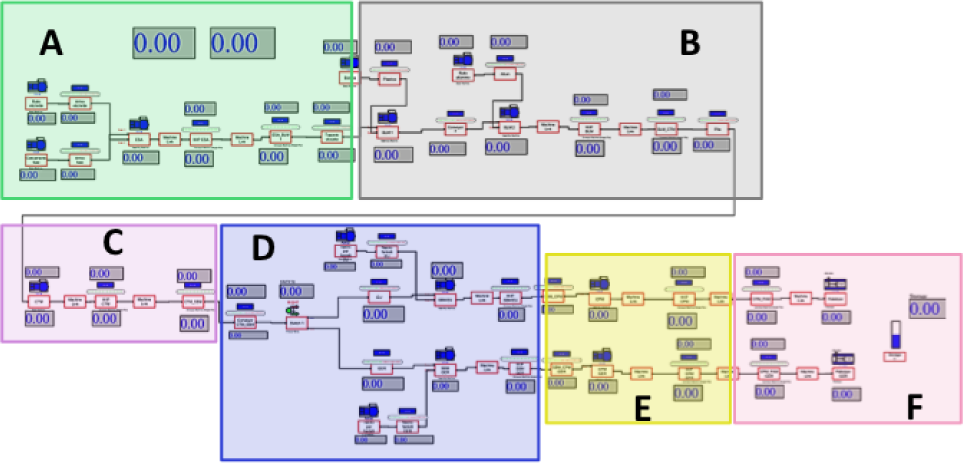
Simulation model of the packaging line. The areas highlighted with different colours identify the parts of the model that define the behaviour of each of the machines that make up the line (A, B, C, D, E, F)
Before using the simulation model, the steps of verification and validation were carried out. The validation was performed considering the different characteristic parameters of the line, by comparing the results provided by the model with the real ones.
Figure 5 shows, as an example, the comparison between the actual and simulated cumulative production of machine C for a specific batch.

Real vs. simulated trend of the cumulative production of a specific batch of the C machine. The real data were obtained from the production log while the simulated data derives from the simulation results.
Referring to Figure 5, Table 4 shows the cumulative production of the C machine both for the real and for the simulated case.
Real vs. simulated trend of the cumulative production, for a specific batch of the C machine. The real data were obtained from the production log, while the simulated data derives from the simulation results.

In the graph, of course, you may not notice any stop for failure, given the relative shortness of the time on the horizontal axis. You can still observe a non-linear trend due to the interaction between the different machines and inter-operational buffers. From the analysis of the two graphs it is clear that the trends are comparable, with an exception for a greater speed in the phases of filling and emptying of the line, visible in the simulation model compared to reality.
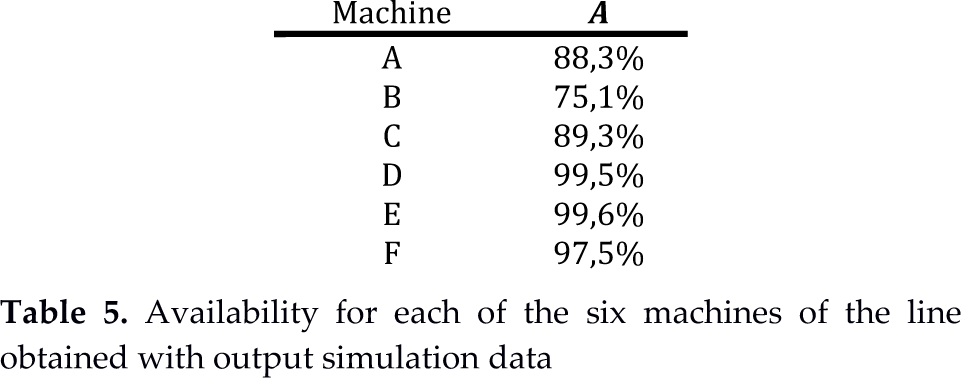
Table 5 shows the value of availability evaluated with the output data of the simulation model.
Availability for each of the six machines of the line obtained with output simulation data
In order to attain a complete representation of the performance, Table 6 shows the availability of the line compared to the results of the simulation model with real data (these are shown in Table 1).
Real vs. simulated availability for the packaging line

The simulation approach allows the non-conformity management typical of the pharmaceutical industry to be taken into account. While in most production or packaging lines quality controls are carried out almost entirely at the end of the process, in the pharmaceutical field they are distributed along the entire line. This is mainly due to the stringent quality controls typical of this area. The stage of packaging, also, as the final link in the chain of making a product, is not suitable for the identification of defective parts at the end of the line, when the products are already contained in boxes and pallets. It is quite necessary that controls on the quality of the product are carried out continuously at intermediate points of the line, so as to identify and discard (or rework) non-compliant pieces as soon as possible. In practice, the quality controls typical of our case study relate to the physical integrity of the vials, the presence of the label of the medicine, the correctness of the number of vials inserted in each package, and so on.
From the operational point of view, the quality values of each machine were introduced by taking them from the experimental values. Availability and performance efficiency were obtained experimentally by the interaction of each station with the other, introducing the setups, the scheduled stops and the reliability and maintainability values of each machine.
The simulation results were very useful for the line managers because, in addition to providing the behaviour of every single machine, they enabled an OEE value to be obtained for the entire production line. The OEE of the entire line obtained by the simulation model is 61.20%.
The simulation results were compared with the real data and with an experimental productivity KPI in use in the company, calculated as the ratio between real and the theoretical productivity. For instance a value of 60% means that the real production is 60% of the maximum theoretical value obtainable. The experimental value is very close to the simulated one, but slightly lower (the value is not given here for industrial confidentiality). The comparison with the company's KPI was the way to verify the quality of both the simulation results and the theoretical methods.
A critical analysis of the results is provided in the next section.
6. Discussion and conclusion
The application of the models presented previously has shown how the simulation approach is more suitable for representing the packaging line considered in this study. The problems related to the application of the OEE models, both classical and its evolutions, in fact, have also been faced in our case study. Although the results of the analytical models are to be considered quite well, simulation, however, makes it possible to obtain results more meaningful to the business because every aspect of the line can hypothetically be considered.
The simulation approach is more demanding than the analytical one: to have a true and reliable model huge effort is necessary, both in terms of time and competency. Most of the time has been spent identifying all the necessary parameters and adjusting the model during the verification and validation phases.
The main element that differentiates simulation by analytical models is the presence of decoupling points along the line. The buffers allow separation of the machines and ensure that they can work independently of each other (i.e., when there are downstream or upstream stops, a machine can work anyway picking up the worked pieces from the upstream buffer and putting them in the downstream buffer).
The analysis of the results (see Figure 5) has shown that the simulation model cannot perfectly represent real production, due to a mismatch between reality and the model in the start-up phase. For this reason the simulation model has been modified in order to give a better representation of the actual functioning of the packaging line. The simulation software used allows definition of speed related to the phases of the opening and closing of batches. This information has been derived through line observation. Introducing these speed values, the differences between the two patterns of Figure 5 are reduced and the pattern adheres to reality even more.
A further comparison can be made by considering the buffer upstream of the bottleneck. Figure 6 shows the trend of this buffer in the real case, while Figure 7 shows its performance in the simulation model.

Number of pieces in the buffer upstream of the bottleneck in the real case

Number of pieces in the buffer upstream of the bottleneck in the simulated case
As well as the model, the OEE value of the entire line changed, passing from the previous 61.20% to the new estimate of 58.80%. Thus, this additional modification of the model has led to further reduction of the gap between the experimental value recorded in the KPI, and the simulation.
With regard to the theoretical models, their predictions have been a bit too far from experimental reality.
The classical OEE calculation gave results that were too low, for the bottleneck of the line, when compared with real data. This is explained by the lack of buffers in the calculation model.
The second model, in addition to not managing the buffers, has worsened the situation because it assumes that scraps proceed along the line without being reworked. As has been stated previously, it takes into account the quality index of every upstream station by reducing it according to the downstream machines, but this is not suitable for our pharmaceutical environment. As a matter of fact in the pharmaceutical industry, as mentioned, the defective parts are identified and immediately extracted from the line with automated procedures.
The third model, lastly, provides a higher value, although the lack of any modelling of the buffer causes a limitation in the reliability of the results.
To sum up, we can say that the classical OEE approach is helpful with individual machines, and the second approach is well suited to scenarios with synchronized and well balanced paced lines, while the third can also manage imbalances of the stations but does not include the effects of buffers.
The simulation, on the contrary, is suitable for modelling any ‘abnormal’ situations and, for this reason, proves to be a valuable alternative to analytical models, especially in all cases in which the system is not reducible to any encoded stereotype.
To conclude, we can say that the availability of performance measures able to assess the efficiency of a production or packaging line is essential for monitoring performance, identifying problems and planning improvement actions. Some measure models are more appropriate than others, because they enable comprehension of more typical elements of the real system.
The analytical methods have proven to always be able to provide some estimate of the production performance of the line. In any case, it is important to be careful in selecting the model and in making assumptions that define its scope. If the choice is well thought out, these methods have significant advantages in terms of speed and effectiveness. If, however, we must investigate in more depth the behaviour of the line, highlighting the mutual relations between the machines and the ways in which they interact with each other and with the inter-operational buffer, then the simulation is the best available approach. Simulation, despite the high expenditure of time and cost, is still today one of the instruments with the greatest effectiveness. Another advantage of simulation is that it is possible to directly edit one of the input values, in order to verify the effects on output, without going through any intermediate evaluation of formulae as required by the theoretical models. Once the model is built, therefore, the support continues with many possibilities for prompt analyses, modification and improvement of the line.
An increased use of theoretical models for the evaluation of the productivity of a line will be possible only when they allow the representation of unbalanced lines, with an inter-operational buffer, operated under policies of scrap and rework (more realistic management for the industrial context.
From the point of view of the originality of this work, we can say that in the scientific literature there are currently no comparisons between OEE, OEEML, other variants of OEE and simulation approaches, neither in the pharmaceutical nor in the manufacturing field.
Considering future developments, this study shows the importance of developing new analytical models that enable representation of the performance efficiency of a production line, also taking into account the buffer effects. It will thus be possible to apply accurate analytical models that, unlike simulators, are much more immediate and can afford better analysis and comparison of the results.