Sage Journals: Discover world-class research

Abstract

In this paper, a novel approach to achieving the independent control of multiple magnetic microrobots is presented. The approach utilizes a specialized substrate consisting of a fine grid of planar, MEMS-fabricated micro coils of the same size as the microrobots (≤ 500 μm). The coils can be used to generate real magnetic potentials and, therefore, attractive and repulsive forces in the workspace to control the trajectories of the microrobots. Initial work on modelling the coil and microrobot behavior is reported along with simulation results for navigating one and two microrobots along independent desired trajectories. Qualitative results from a scaled-up printed circuit board version of the specialized substrate operating on permanent magnets are presented and offer proof-of-concept results for the approach. These tests also provide insights for practical implementations of such a system, which are similarly reported. The ultimate goal of this work is to use swarms of independently controlled microrobots in advanced, additive manufacturing applications.

Keywords

Mobile Microrobotics Multi-robot Control Additive Manufacturing

1. Introduction

Flexible manufacturing capabilities have been advancing steadily over the years. The resolution and size of the features has improved, and additive manufacturing has proven to be a disruptive technology at the small- to medium-scale. Many technical challenges exist to extending this technology to micro-scale structures. The ultimate goal of this work is to produce a flexible manufacturing microrobot platform to perform the micro-scale additive manufacturing of smart devices and structures. The state-of-the-art in micro-scale manufacturing does not allow for very complex structures to be created without many costly manufacturing steps. A particular unmet need is for micro-scale manufacturing processes that allow for the assembly of optimal, arbitrary material combinations and geometries. Topology structural optimization codes (genetic algorithms, simulated annealing) often arrive at optimal solutions that are not manufacturable within current capabilities. The potential for small-scale active devices and sensors has driven the investment of a large amount of federal resources into basic material development. The result is that there are now many small-scale building blocks that can be assembled into multi-functional micro-scale devices, structures and sensors. Microrobot manufacturing swarms, assembling and joining multi-functional building blocks, represent an enabling technology that can make this possible and mark the vision for our work. Such a platform has applications across a wide range of domains, e.g., in micro vehicles, steerable catheters, optimal structures, microfluidic circuits and energy harvesters.

2. Related Work in Mobile Microrobotics

Wireless, sub-millimetre mobile microrobots have emerged with new capabilities, operational modes and high operational speeds - when compared to traditional robots - facilitated by their small size and mass. As such, mobile microrobots with these features are likely to have a major impact in biology and advanced manufacturing applications in the future [1]. The main challenge in realizing a mobile microrobot is constructing an effective power storage and locomotion system [2]. Representative power and actuation mechanisms applied to mobile microrobots include electrostatic [3, 4], thermal and optical [5 –9], piezoelectric [10], biological [11 –14], electromagnetic [15 –17], and combined piezoelectric-electromagnetic [18] approaches. Electromagnetic systems using external magnetic fields provide attractive merits and offer the most promising results to date for untethered mobile microrobots [15, 16]. Some systems use external magnetic field gradients to propel the magnetic microrobots [19, 20]. Magnetic force-scaling depends on both the distance and the agent volume, and therefore this type of propulsion requires relatively large magnetic fields. Torques or non-gradient magnetic fields induced on magnetic bodies have led to a variety of microrobot locomotion concepts. In [21], microrobots consisting of neodymium-iron-boron (NdFeB) magnetic bodies are controlled with low-frequency magnetic fields to induce stick-slip locomotion of the body in order to achieve real-time controlled movement. A similar approach is proposed for biomanipulation in [22]. Rotating magnetic fields have also been utilized to drive helical microrobots to swim in low Reynolds' number regimes [23 –25]. A wireless resonant magnetic microactuator Magmite family of microrobots has been developed in [15, 26] using oscillating magnetic field actuation.

Similarly, in [27 –31], the fabrication, magnetic powering and control of wireless mobile microrobots operating on both dry surfaces and in aqueous environments has been demonstrated. Three families of mobile microrobots have been built: micro-scale magnetostrictive asymmetric bimorph (μMAB) microrobots, soft magnetic body (SMB) microrobots and micro-scale tumbling (μTUM) microrobots. The magnetic nickel layer of the μMAB is designed to expand and contract in the presence of an oscillating magnetic field, resulting in drive forces under the front and rear feet of the robot. Due to its asymmetric design, it locomotes in the direction of the front (i.e., the larger) feet. On the other hand, the SMBs are designed specifically for operation with gradient magnetic fields, with the robot translating along the direction of the field lines. The μTUM robots are designed in a dumbbell structure, consisting of two oppositely poled permanent magnet bells attached with a connection bar. It has two locomotion modes: tumbling mode and a sliding, stick-slip operating mode.

External electromagnetically powered microrobots require the same control signal to be sent to all of the microrobots in the workspace. Control strategies for this situation exist, but the tasks that can be achieved by multiple agents are limited by various constraints, such as a low number of agents (not scalable), non-smooth trajectories, coupled robot behaviours, and the robots meeting in the same location, congregating close together or colliding, while some are only realizable in fluidic environments [32 –40]. In some cases, the control strategies assume microrobot capabilities that are not yet realizable in practice [41]. If mobile microrobots are to be used outside of a controlled laboratory setting and for actual manufacturing tasks, future work on developing technologies to facilitate the operation and control of multiple microrobots is necessary. In this paper, we present our unique approach and initial work on obtaining the independent control of multiple magnetic microrobots for eventual use in additive manufacturing applications.

3. Technical Approach

3.1 Overview

Artificial potential field navigation controls are a very popular technique for the decentralized control of swarms of macro-scale mobile robots. This method directs a robot as if it were a particle moving in a gradient vector field. Gradients are viewed as forces acting on a positively charged particle robot which is attracted to the negatively charged goal. Obstacles also have a positive charge which forms a repulsive force directing the robot away from them and towards the goal [42]. It is desirable to use this technique at the micro-scale to control 2D swarms of microrobots. This can be done by generating real local (magnetic) potential fields at a fine resolution through the use of a specialized substrate consisting of MEMS-fabricated planar micro-coils (Figure 1). This system will allow for the truly independent and coordinated control of mobile magnetic microrobots. Real magnetic potential field navigation controls will be developed for both individual control and swarm control of the microrobots by the control substrate. Ultimately, a swarm of magnetic microrobots with specific functionalities for different micro-scale manufacturing tasks will be designed and fabricated along with a set of specialized micro-scale modular blocks and connectors so as to allow the microrobot swarm system to construct a variety of micro-scale devices. These modular blocks will have different material properties, while the connecting pins can have various functionalities. This will enable many advanced additive manufacturing applications.

Figure 1.

Technical approach: a specialized magnetic potential field-generating substrate made from MEMS-fabricated planar micro-coils will be used for the independent control of multiple mobile microrobots for advanced manufacturing tasks

3.2 Motion Primitives

Traditional motion planning in robotics is concerned with the problem of moving an object from an initial configuration to a goal configuration. The goal here is to plan motion paths for a team of microrobots required to perform a number of manipulation and assembly tasks. For this, MEMS-fabricated planar micro-coils will be used to control the magnetic force fields in the workspace. The magnetic forces applied to the magnetic microrobots have the potential to drive the robots to desired locations in the free space. The two main motion primitives that we require from a microrobot to accomplish these tasks are translation and rotation. With a sufficiently fine grid of micro-coils on the substrate, these primitives can be executed in the following ways:

Translation. Translational motion for a single microrobot can be achieved by inducing a positive (repulsive) potential at the starting location of the microrobot along with an attractive (negative) potential at its goal location. This will generate magnetic force vectors in the workspace of the microrobot, propelling it along a straight-line trajectory from its initial position to its goal position. A similar procedure can be followed in order to generate magnetic potential fields for more complex translational motion primitives for more than one robot and/or goal location (Figure 2(a)). In addition, with individual control of all the coils in the substrate, a swarm of microrobots can also be translated in the free workspace while maintaining a desired formation. As long as the relative distance between the positive and negative potentials holds, this formation will remain intact. Therefore, different coils in the substrate can be activated/deactivated with this same pattern in order to translate the microrobots in this formation along the substrate.

Figure 2.

Mobile microrobot motion primitives. (a) Translation: Two microrobots to two goal locations; (b) and (c): Rotation.

Rotation. The specialized substrate will also be able to rotate microrobots of interest. It can do this by changing the relative position of the potentials around the microrobot, as shown in Figure 2(b) and (c). In this scenario, a repulsive (positive) potential is held stationary under the robot while an attractive (negative) potential is rotated around the positive potential counter-clockwise. This results in the counter-clockwise rotation of the microrobot. The negative potential can be generated and rotated in the opposite fashion for rotation in the clock-wise direction.

4. Modelling for Microrobot Navigation using Magnetostatic Forces

In order to realize such a system as described in Section 3, we start with the modelling of the magnetic field and forces that such a specialized substrate of micro-coils can generate and examine whether it is feasible for use in controlling the trajectories of a magnetic microrobot. This modelling is presented next.

4.1 Designing Magnetic Fields

The currents which arise due to the motion of charges are the source of magnetic fields. When a current is passed through a circular coil, a magnetic field is produced around it. The strength of the magnetic field produced by a current-carrying circular coil can be controlled by:

Increasing/decreasing the current flowing through the coil

Increasing/decreasing the number of turns in the coil

Modifying the coil geometry, such as the diameter, width, winding/turn spacing, etc.

To calculate the magnetic field due to a circular current loop at a generic point P in space (Figure 3), one can first examine the magnetic vector potential:

Figure 3.

A circular current loop generating a magnetic field at an off-axis point P [43]

A = \frac{μ_{0} I}{4 π} \oint ​ \frac{d l}{s} .

(1)

where μ₀ is the permeability of free space, I is the current flowing through the coil, dl is the differential element carrying current I, and s is the distance from the current source to the field point P.

Using cylindrical coordinates at the point P(r,θ,z) and following [43, 44], the magnetic potential at point P can be written as:

\begin{array}{l} A = \frac{μ_{0} I \sqrt{R}}{2 π} [2 k^{- 1} r^{- 1 ∕ 2} E_{1} (k) \\ - 2 k^{- 1} r^{- 1 ∕ 2} E_{2} (k) - k r^{- 1 ∕ 2} E_{1} (k)] {\hat{e}}_{ϕ} \end{array}

(2)

where R is the radius of the circular coil and ${\hat{e}}_{ϕ} = - \hat{i} \sin ϕ + \hat{j} \cos ϕ$ , and where:

E_{1} (k) = \int_{0}^{π ∕ 2} \frac{d θ}{\sqrt{1 - k^{2} \sin θ^{2}}}

(3)

is the complete elliptic integral of first kind:

E_{2} (k) = \int_{0}^{π ∕ 2} \sqrt{1 - k^{2} \sin θ^{2}} d θ

(4)

is the complete elliptic integral of second kind, and:

k^{2} = \frac{4 r R}{z^{2} + {(R + r)}^{2}}

(5)

The magnetic field at point P(r,θ,z) is then:

\vec{B} = \nabla \times \vec{A}

(6)

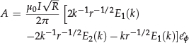
with the two components of the magnetic field along the z and r axes expressed as:

B_{z} = \frac{μ_{0} I}{2 π \sqrt{z^{2} + {(R + r)}^{2}}} (\frac{R^{2} - z^{2} - r^{2}}{z^{2} + {(r - R)}^{2}} E_{2} (k) + E_{1} (k))

(7)

B_{r} = \frac{μ_{0} I z}{2 π r \sqrt{z^{2} + {(R + r)}^{2}}} (\frac{R^{2} + z^{2} + r^{2}}{z^{2} + {(r - R)}^{2}} E_{2} (k) - E_{1} (k))

(8)

When modelling planar micro-coils analytically, spiral coils can be represented by concentric circles [45]. The magnetic fields for each concentric circle can then be added up to approximate the total flux resulting from the entire coil. The planar geometry of the coil determines the number of concentric circles needed for the calculation and the coil winding cross-sectional dimensions are used to determine the allowable currents that can be applied.

To obtain a fine resolution of the magnetic potentials in the workspace, it is desirable to have the size of the micro-coils as either the same size or else smaller than the microrobots (≤ 500 microns). From the work in [31], experiments show that the static force needed to move a micro-scale robot on a dry surface from rest is of the order of 5 μN, corresponding to a magnetic field strength of about 1 mT.

A planar micro-coil model with an outside diameter of 300 μm, a planar winding width of 7 μm, an out-of-plane winding thickness of 7 μm and a winding spacing of 7 μm, producing a micro-coil with 10 turns with an input current of 150 mA (in free air), was analysed as shown in Figure 4. At a distance of about 25 μm from the center of the micro-coil, a magnetic field intensity of approximately 1 mT is generated.

Figure 4.

Single planar micro-coil analysis. A 10 turn micro-coil with an outside diameter of 300 μm and an input current of 150 mA will produce a 1 mT magnetic field intensity approximately 25 μm from the center of the coil.

The magnetic field strengths for a cluster of micro-coils are examined next, as we want to control multiple micro-coils on the substrate at the same time in order to navigate the microrobots. A schematic of a seven-coil cluster arrangement is shown on the left of Figure 5. Each coil has an identical geometry, as in the previous single coil analysis. Here, some coils have positive input currents (repulsive potentials) while some have negative input currents (attractive potentials). The values for the currents for each coil are also listed in the figure. The 3D plot of the magnetic field on the right of Figure 5 shows that a magnetic field of approximately 1.5 mT is able to be generated above Coils 2, 5 and 7, while the fields residing along the other coils are substantially lower for these settings. A field such as this can be used to repel a robot from Coil 2, 5 or 7 to another location of lower potential. It can also be used as a barrier between a microrobot on Coil 1 or 3 and a microrobot on Coil 4 or 6 to prevent them from getting too close together. A more detailed analysis of how the magnetic fields generated by this coil cluster can be used to control the path of a microrobot is shown in Figure 6. Here, a microrobot is presumed to start outside of the magnetic coil cluster region. Attractive potentials are generated at Coils 2, 5 and 7 to move the robot to the cluster (Figure 6(i)). Next, the attractive potentials remain on at Coils 2 and 7 while the repulsive potentials are created at Coils 3 and 6 (Figure 6(ii)). Coil 2 is then set as the only attractive potential with repulsive potentials at Coils 3, 5 and 6 (Figure 6(iii). Finally, with the attractive potential still at Coil 2, repulsive potentials at Coils 3, 5, 6 and 7 will be able to generate enough field strength to move the robot to Coil 2 (Figure 6(iv)).

Figure 5.

Micro-coil cluster analysis. A seven-coil arrangement of 10 turns, 300 μm diameter micro-coils with the input currents specified is able to generate enough magnetic field to repel a robot from one coil and onto a neighboring coil. It can also serve as a barrier to keep microrobots separated on the substrate.

Figure 6.

Micro-coil cluster analysis for microrobot navigation from Coil 5 to Coil 2. (i) A microrobot is presumed to start outside of the magnetic coil cluster region and attractive potentials are generated at Coils 2, 5 and 7 to move the robot to the cluster. (ii) Attractive potentials remain on at Coils 2 and 7 while repulsive potentials are created at Coils 3 and 6. (iii) Coil 2 is the only attractive potential with repulsive potentials at Coils 3, 5 and 6. (iv) Finally, with the attractive potential still at Coil 2, repulsive potentials at Coils 3, 5, 6 and 7 will be able to generate enough field strength to move the robot to Coil 2.

4.2 Designing Magnetic Navigation Forces

In order to determine if the approximately 1 mT field strength will be able to be used to control the trajectories of the microrobots, we need to consider the geometry and properties of the microrobot itself and the resulting magnetic forces on the microrobot from the prescribed fields. We can consider the microrobot to be a permanent magnet that is poled through its thickness direction (north pole at the top, south pole at the bottom, or vice versa). We can model this as a magnetic dipole. If a magnetic dipole is placed at point P, due to the non-uniformity of the magnetic field, the dipole will experience a force given by:

{\vec{F}}_{B} = \nabla (υ \cdot B) = υ_{r} \frac{d B_{r}}{d r} \hat{i} + υ_{z} \frac{d B_{z}}{d r} \hat{k}

(9)

where υ_r and υ_z are the two components of the permeability of the material of the dipole. This force can be either attractive or repulsive, depending on the direction of the dipole.

Using Newton's difference quotient, $\frac{d B_{r}}{d r}$ and $\frac{d B_{z}}{d r}$ can be calculated numerically. The difference between two points is known as their Delta (Δr). The function difference divided by the point difference is known as the difference quotient. Thus, we can write:

\frac{Δ B (r)}{Δ r} = \frac{B (r + Δ r) - B (r)}{Δ r}

(10)

If Δr is infinitesimal, then the difference quotient is a derivative.

Consider a square cell with four coils, one in each corner as shown in Figure 7. The microrobot is modelled as a “point” about its center of mass. The total magnetic force in the z-direction is the algebraic sum of the F_z values of the four coils. The F_r values generated by each coil are decomposed into the global (microrobot) coordinate system (X and Y) components, and the total forces in the x- and y-directions from the coil set are calculated as the sum of the x and Y components from each coil, accordingly. Finally, we can write the resultant magnetic force on the robot from the set of four micro coils as F_x, F_y, and F_z.

Figure 7.

Resultant magnetic forces generated at point P by a set of four micro-coils The net force in the z-direction, F_z, is simply the sum of the z-direction forces generated by each coil at point P. The r-direction forces for each coil are decomposed into x- and y-direction components and then added together along each of these axes to produce the net magnetic force in the x- and y-directions (F_x and F_y) on the robot.

The trajectory of the robot can be determined taking the resultant force on the robot F_total and Newton's second law of motion as:

a (q) = \frac{F_{t o t a l} (q)}{m}

(11)

where a is the acceleration due to the resultant force F_total, m is the mass of the microrobot and q is the discretized state of the system. From this equation of motion, we can also determine the corresponding microrobot velocity:

υ (q) = υ (q - 1) + a (q) Δ t

(12)

where υ(q) is the velocity of the robot, υ(q − 1) is the initial velocity of the robot and Δ t is the time step. For q=1, υ(0) = 0, and so we can write the position x of the microrobot as:

x (q) = υ (q - 1) Δ t + \frac{1}{2} a (q) Δ t^{2}

(13)

With a microrobot starting from rest, it will need to overcome static friction. The static friction can be written as:

F_{s} = μ_{s} N = μ_{s} [W - F_{z}]

(14)

where μ_s is the static friction coefficient, N is the normal force, W is the weight of the robot and F_z is the total magnetic force in the z-direction. Once the robot starts to move, it will need to overcome the dynamic friction. This is described by:

F_{k} = μ_{k} N = μ_{k} [W - F_{z}]

(15)

where μ_k is the dynamic friction coefficient.

Therefore, the trajectory of the robot can be determined using Eq. 11 with the total force on the robot, F_total, written as:

F_{t o t a l} = F_{x y} - F_{s}

(16)

when υ(q) = 0 and:

F_{t o t a l} = F_{x y} - F_{k}

(17)

when υ(q) ≠ 0. Here, F_xy is the resultant force in the x/y-plane exerted on the microrobot by the coils, as determined from F_x and F_y. Therefore, the robot will start to move when F_xy > F_s and it continues to move until υ(q) = 0.

5. Simulation Results

The goal here is to be able to use a grid of planar micro-coils to control individual microrobots with arbitrary trajectories. Now that the equations of motion for the magnetic microrobot have been established along with the magnetic force capabilities of the micro-coils, we can simulate the coil inputs needed to obtain some desired trajectories of the microrobot for a given micro-coil grid configuration.

Figure 8 shows a schematic of the coil configuration used in the simulations. It is a 4×4 grid of 16 micro coils, each spaced 500 μm - both horizontally and vertically - from each other. The outside diameter of the coils is 80 μm and there are two turns for each coil. A permanent magnetic robot made of neodymium is used with dimensions of 300 μm × 300 μm × 250 μm, also shown schematically in Figure 8. When the microrobot is located in a region in the workspace that overlaps with the position of a coil, the coefficients of static and dynamic friction for this metal-metal contact are μ^metal_s = 0.3 [46] and μ^metal_k = 0.15 [47], respectively. When the microrobot is in a region that does not overlap with the position of a coil, a metal-plastic contact is assumed and coefficients of the static and dynamic friction of μ^plastic_s = 0.25 and μ^plastic_k = 0.10 are used, respectively [48].

Figure 8.

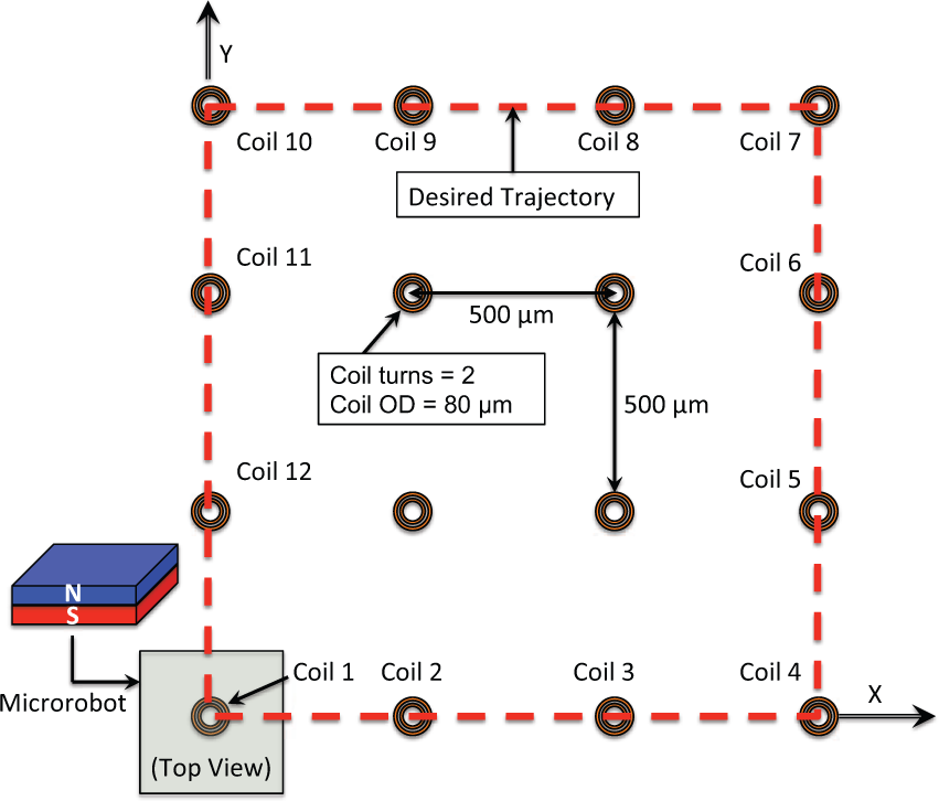
Schematic showing microrobot and a 4×4 grid of micro-coils used to navigate the microrobot along the desired trajectory (red). The microrobot starts from rest in the location shown and then moves with a constant velocity of 200 mm/s along the path in a counter-clockwise direction.

In the following simulations, we perform open-loop control of the microrobots. The current state of the robot and the model of the system are used to determine the applied force needed to drive the microrobot to a desired point (a waypoint or a final point). The required current inputs for the micro-coils are then solved to produce the appropriate forces in the workspace. As this controller is open-loop, it is not robust to disturbances. This means that any disturbances due to the environment or unmodelled dynamics in the system will drive the robot to a different position from the desired position. For these simulations, ideal conditions without any disturbances are assumed. Therefore, the actual and goal robot trajectories are identical.

5.1 Single Microrobot Trajectory Aligned with Coils

In the first case examined here, the desired trajectory of the microrobot is a 1.5 mm × 1.5 mm square path directly on top of the coils on the grid. This is shown at the red line in Figure 8. The microrobot starts from rest at the location of Coil 1 and then travels at a constant velocity of 200 mm/s along the path in a counter-clockwise direction. A time step of 10⁻⁵ seconds is used and a linear program is utilized to compute the appropriate bounded current values that meet the magnetic force requirement to move the microrobot the desired distance during the prescribed time step along the desired trajectory (waypoint control). The current values are limited to maximum/minimum values of ±500 mA. Figure 9 shows the current levels in the coils as the robot moves along the path from Coil 1 to Coil 4. For this trajectory, only those two coils that the microrobot is navigating from and towards are needed to control its movement. For example, when the robot is translating laterally between Coils 1 and 2, an attractive force (+ current values) is generated at Coil 2 while a repulsive force (− currents values) is needed at Coil 1 (Figure 9(top)). Similarly, when the robot moves between Coil 2 and Coil 3, Coil 1 is turned off and attractive forces are generated by Coil 3 along with repulsive forces emanating from Coil 2 (Figure 9(middle)). The same pattern holds for when the robot moves between Coil 3 and Coil 4 (Figure 9(bottom)). Next, the direction of the robot must change in order for the robot to start to move in the y-direction towards Coil 5. As the microrobot continues to navigate its way along the path, the same current patterns emerge as each additional segment of the path is a straight-line path between two coils.

Figure 9.

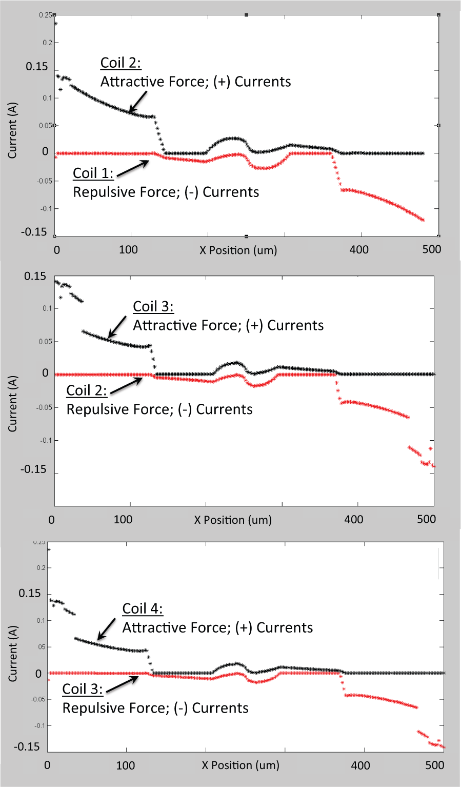
Coil current levels as a function of the microrobot position along the x-axis for a microrobot trajectory aligned with the grid of micro coils

5.2 Single Microrobot Trajectory Misaligned with Coils

Obviously, it is not feasible to expect all the desired trajectories for the microrobot to reside directly above the coil locations on the substrate. Therefore, the issue of how to determine the appropriate coil current levels for a square path that does not overlap the coil locations is examined next. Figure 10 shows the schematic for this simulation. The same coil geometry used in the previous example is used along with a with 750 μm spacing along with the same microrobot geometry and polarity and friction coefficients. The desired path shown in red is now 2.1 mm × 2.1 mm in size. The robot starts from rest in the lower left corner of the path and is then required to traverse the path in a clockwise fashion with a constant velocity of 200 mm/s. The step size is 10⁻³ seconds. Now, instead of just using two neighboring coils to control the position of the robot along the path, sets of four coils are used at a time, creating a rectangular active coil region to control the position of the microrobot. For example, to get the microrobot to move from its starting location an active coil region consisting of Coils 1, 2, 3 and 4 is utilized. Coils 1 and 2 generate repulsive forces on the robot (− currents) while Coils 3 and 4 generate attractive forces on the robot (+ currents). The current levels for the coils in the active coil region are shown in Figure 11(top) as a function of the position of the microrobot. Once the x-position of the microrobot gets to the x-position of Coil 3 (Coil 4) on the grid, the active coil region switches and consists of Coils 3, 4, 5 and 6. Next, Coils 3 and 4 apply repulsive forces while Coils 5 and 6 apply attractive forces to the microrobot (Figure 11(middle)). The same pattern continues as the x-position of the microrobot passes the x-position of Coil 5 (Coil 6) on the grid with Coil 5 and Coil 6 generating repulsive forces and Coils 7 and 8 generating attractive forces (Figure 11(bottom)). Again, large accelerations will occur at the corner point of the trajectory where the 90° change of direction occurs. After the robot reaches the corner position, the active coil region will remain the same but now Coil 5 and Coil 7 will generate the repulsive forces and Coil 6 and Coil 8 will generate attractive forces to navigate the robot along the y-direction. As the microrobot continues to navigate its way along the path, the same current patterns emerge for the active coil regions consisting of the four neighboring coils of the microrobot.

Figure 10.

Schematic showing the micro-coil grid and a desired microrobot trajectory that is not aligned with the coil grid. The microrobot starts from rest at the lower left corner of the path and then traverses it in a counter-clockwise manner with a constant velocity of 200 mm/s. Sets of four neighboring coils are used to create an active coil region to control the position of the microrobot along the corresponding section of the path.

Figure 11.

Coil current levels as a function of the microrobot position along the x-axis for a microrobot trajectory that is not aligned with the grid of micro coils

Note that in both the simulation cases presented, the desired microrobot trajectory is given as the input to the system in order to determine the actual coil input currents. Therefore, the actual and goal robot trajectories are one and the same. The constant velocity constraint is met along both trajectories except at the corner points where the 90° turn is encountered. In these instances, there is an instantaneous spike in the acceleration (rather than it remaining at zero as is the case for a constant velocity). In practice, the robot would need to slow down in order to negotiate this sharp turn instead of holding the constant velocity constraint enforced here.

5.3 Multiple Independent Microrobot Trajectories

When examining the case of generating the appropriate current inputs to the micro-coils for obtaining independent trajectories for multiple magnetic microrobots at the same time, the radius of influence for the micro-coils must be studied. The radius of influence, R_I, for a coil corresponds to the maximum distance away from the coil where the magnetic field is strong enough to induce the movement of the microrobot. If the microrobot is at a distance greater than R_I from the center of the micro-coil, the magnetic field produced by the coil will not cause it to move. For the micro-coil geometry considered here, R_I is directly proportional to the input current to the coil and is listed in Table 1.

Table 1.

Radius of influence of the micro-coils


Input Current (A)	Radius of Influence (μm)
0.1	180
0.2	238
0.3	277
0.4	306
0.5	330

It is easiest to visualize the effects of the coil radii of influence for the case when multiple microrobot trajectories are desired that are aligned with the coil positions (as considered in Sec. 5.1 above). We can construct an influence region around the two active coils used to move a particular microrobot to/from the waypoints located above these respective coils by conservatively using the largest R_I value in Table 1, corresponding to the maximum allowable input current (330 μm). This can be done for every microrobot in the workspace that is to be controlled. Figure 12 illustrates these regions for three different microrobots in the workspace. The region of influence is created by first drawing circles with diameters corresponding to d = 2 × R_I around each coil. Lines tangential to these circles are then constructed to connect the two circular influence regions into one continuous slot-shaped influence region. As long as there are no overlapping influence regions for all the desired microrobot trajectories in the workspace, one can proceed to generate the required current inputs in the exact same manner as was done in Sec. 5.1. In fact, the input current profiles will be identical to those shown in Figure 9. This scenario corresponds to trajectories with at least one micro-coil separation between them (500 μm).

Figure 12.

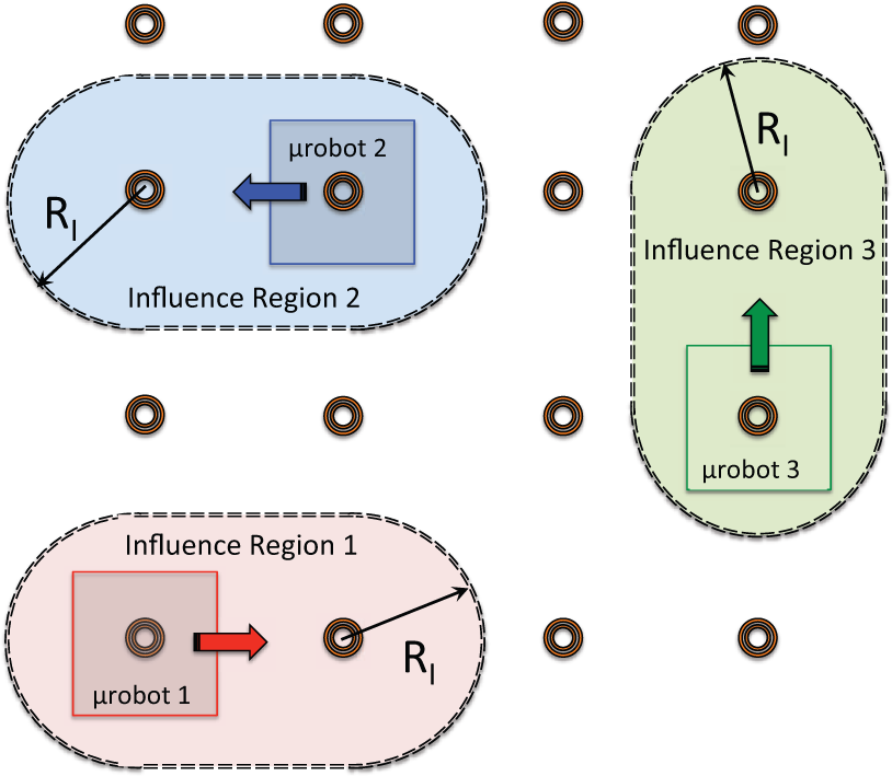
Micro-coil influence regions when controlling three microrobots at the same time with desired trajectories aligned with the micro-coil locations. As long as the influence regions for the different microrobots do not overlap at the same time, the independent control of each microrobot is possible.

The influence regions for all the desired microrobot trajectories can actually overlap as long as they do not overlap at the same time. For example, the microrobots can have a shared waypoint but they cannot be there at the same time. The scheduling of which robot is to go to which particular location needs to be taken into account during trajectory planning, which is a topic of our future work.

When the microrobots in the workspace have desired trajectories that are not aligned with the coils, as discussed in Sec. 5.2, one can employ as similar approach as just described. Instead of just two coils contributing to the influence region, the four active coils will create the influence region. Instead of being slot-shaped, it will be rectangular in nature with rounded corners, with the radius corresponding to the R_I value (Figure 13). For this scenario, the input current profiles for the coils in the influence region will be identical to those shown for the active coils in Figure 11. Again, trajectories that do not have overlapping influence regions at the same time can be utilized to obtain the independent control of multiple microrobots.

Figure 13.

Micro-coil influence regions when controlling two microrobots at the same time with desired trajectories that are not aligned with the micro-coil locations

Note that for the discussion here in Sec. 5.3, it is assumed that the radius of influence between adjacent magnetic robots (the distance that will cause the two magnets to stick to each other) is smaller than R_I. This is a reasonable assumption for two magnetic dipoles of the size used here with parallel magnetic pole directions.

To plan the motion of multiple microrobots, we employ a similar open-loop controller to that used in Sections 5.1 and 5.2. Unlike the discussion in those sections - which decompose the desired microrobot trajectories into waypoints and adapt the coil currents so that the microrobot tracks those desired waypoints - we here simulate a simpler situation where the desired microrobot trajectory is defined by an initial and a final position, under the assumption that constant currents exist that can realize this trajectory. This is without loss of generality, as the purpose of this experiment is to test the independent motion of multiple robots in close proximity to each other. For richer trajectories that cannot be realized by constant coil currents, a similar approach to Sections 5.1 and 5.2 can be employed with the decomposition of these trajectories into appropriate waypoints. In what follows, a simulation of two microrobots that need to track the desired trajectories that can be realized by constant coil currents is presented. We show that the proposed framework is able to achieve independent robot motion as desired.

To examine the constant current case, one can utilize the equations presented in Sec. 4 and the concept of the radius of influence for the micro-coils. Consider a grid of eight micro-coils with 500 μm spacing, arranged as shown in Figure 14. Coils 1 through 4 create an active coil region to control the position of Microrobot 1 as it traverses a path inside this region. Similarly, Coils 5 through 8 create an active coil region to control the position of Microrobot 2 as it moves through this region. A coil region - or cell - consisting of Coils 3 through 6 makes up a buffer region ensuring that the regions of influence for the active coil regions for Microrobot 1 and Microrobot 2 do not overlap.

Figure 14.

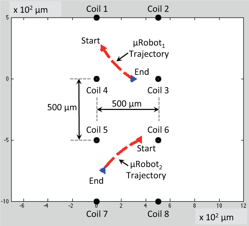
Two independent microrobot trajectories resulting from a constant input current in the micro-coils. Such input results in curvilinear trajectories that can be adjusted to control which side of the active coil region the microrobot will exit.

For the simulated microrobot trajectories shown in Figure 14, the same microrobot and coil geometry as well as the friction coefficients used previously are used. All the coils are prescribed constant positive current values to create attractive forces on the robots. The constant current values for Coils 1 to 4 are 0.01 A, 0.20 A, 0.40 A and 0.30 A, respectively. The current values for Coils 5 to 8 are 0.20 A, 0.01 A, 0.40 A and 0.20 A, respectively. The initial position for Microrobot 1 is halfway between Coil 1 and Coil 4 on the left side of the active region. The initial position for Microrobot 2 is between Coils 5 and 6 at the top of its active coil, closer to Coil 6 than Coil 5. The constant current input into the coils results in independent curvilinear trajectories for each microrobot. The simulation stops when each robot reaches the border of its active region. Microrobot 1 exits its active region between Coil 3 and Coil 4. Microrobot 2 exits its active region between Coils 5 and 7. Adjacent regions consisting of four micro-coils can be actuated to continue the robot along a desired trajectory through the region. The value of the current in the coils can be adjusted to cause the microrobots to exit their active region at any side (i.e., the goal face).

6. Experimental Observations

A scaled-up printed circuit board (Figure 15) consisting of an 8×8 grid of planar coils was manufactured to perform proof-of-concept studies and to check the validity of the modelling and simulation results presented previously. Two double-channel high-power (375 W) power supplies were used to apply positive and negative currents to the coils on the substrate. The microrobots were approximated by several different-sized permanent magnets that were poled through their thickness, as shown in Figure 8. The magnetic field strengths were measured with a Gauss meter.

Figure 15.

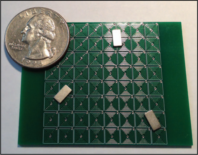
Printed circuit board version of the specialized substrate of planar coils and three permanent magnets. This 8×8 array of 5 mm square coils with five turns is used with magnets of different sizes for qualitative experiments.

Various kinds of experiments were carried out to analyse the different behaviours of the microrobots. The effects of the magnetic field due to the current flowing in the conductive coils and its interaction with the magnet were studied in detail to figure out the best possible method for actuating (exciting) the coils for the appropriate locomotion of the magnets. The following are descriptions of the tests performed, the qualitative results and the conclusions drawn based on these results.

6.1 Coil Excitation Tests

6.1.1 Single Coil Excitation

Setup: A magnet as placed on the particular coil to be excited.

Result: When placed biased to one particular side of the coil, the magnet was attracted to the center of the coil but, in some cases, the force was not large enough to result in any movement. On the other hand, when the magnet was flipped-over, changing its polarity, the magnet was repelled away from the coil for the same current setting and starting location. This result can also be obtained by changing the direction of the current through the coil instead of flipping the magnet.

6.1.2 Two Coil Excitation

Setup: A magnet was placed on one coil that was to be excited. A coil neighboring the first coil was also excited.

Result: Similar results to the previous case were obtained. However, the movement of the magnets was better-directed towards the neighboring (destination) coil which was also excited and providing an attractive force (unlike the random direction in which the magnet was moved in Case 1).

6.1.3 Multiple Coil Excitation

Setup: The magnet was placed on one coil to be excited with a repulsive force. A neighboring destination coil to the right was excited with an attractive force. Auxiliary coils around the starting and destination coils were also excited to ensure the well-directed movement of the magnet.

Result: Much better results were obtained in this scenario. This was because the repulsion forces from the auxiliary coils ensured that the tendency of a magnet to drift away towards other coils was restricted. Hence, it tended to move only towards the destination coil.

Conclusions: The coil excitation tests confirm that the coils are able to produce attractive and repulsive forces strong enough to generate the movement of a permanent magnet of a similar size. It is difficult to precisely control the movement of the magnet using just two coils. The more coils that are used, the easier it is to direct the motion of the magnet from the source to the destination coil. Figure 16(a) shows the minimum number of auxiliary coils that should be used for the movement of the magnet from the starting cell to green destination cell based on these tests. The yellow cell indicates the repulsive forces of the coils, while the green cell corresponds to attractive forces being applied. The best possible configuration to ensure directed movement from the starting location to the destination cell is shown in Figure 16(b). In practice, the optimal number of coils to be excited will be based on a number of other system parameters.

Figure 16.

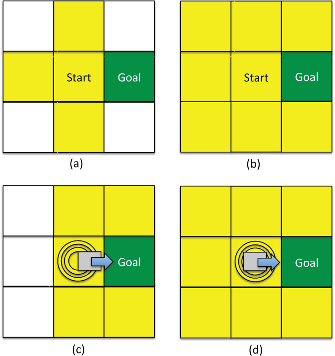
Coil states for magnet translation. Yellow = repulsive force, green = attractive force. (a) Auxiliary coils at the top, bottom and to the left of the starting coil can be used to help direct the magnet to the goal location. (b) Additional auxiliary coils turned diagonally to the starting coil can increase the reliability of the magnet translation. (c) Biased positioning of the magnet and coil settings to translate it to the goal coil. (d) Centered position of the magnet on the starting coil and coil settings used to more reliably direct the magnet to the goal coil.

6.2 Current Modulation Tests

6.2.1 Changing the Current Direction

Setup: A magnet was placed on a coil to be excited. The direction of the current flowing through the coil was altered.

Result: For one direction of current, the magnet experienced an attractive force whereas for the opposite direction it experienced a repulsive force. The magnetic field produced due to the current was verified using a Gauss meter.

6.2.2 Varying the Current Magnitude

Setup: A magnet was placed on a coil to be excited. The magnitude of the current was varied, both gradually and abruptly.

Result: When the magnitude of the current was varied abruptly, the magnet behaviour was very erratic and it had a tendency to flip over. This was because the sharp change in magnetic field strength resulted in an instantaneous magnetic torque pulling the top face of the magnet towards the substrate. A gradual change in the current magnitude gave more consistent results. The magnitude of the currents (0.04–0.20 A) needed to induce movement varied depending on the size of the magnets. The tolerance of the coil (maximum current without burning the coil) with which experiments were carried out was about 2 A.

6.2.3 Current Excitation Timing Effects

Setup: A magnet was placed on a starting (source) coil. The timings for when to excite the source, destination and auxiliary coils were varied.

Result: The most successful results were obtained when the attractive destination coils were excited before the repulsive source coils. Furthermore, the auxiliary coils should be excited slightly before the repulsive force is generated at the source coil. This ensures that all the coils necessary for guiding the magnet will be ready before the “push” from the source coil is generated.

Conclusions: The direction of current controls the type of magnetic force applied to the magnet, with a larger magnitude corresponding to larger forces. However, the speed of change in magnitude administered to the coil as well as the timing of when to excite different coils on the substrate are also crucial factors in obtaining the smooth and controllable motion of the magnet.

6.3 Magnet Positioning Tests

6.3.1 Biased Towards the Destination Coil

Setup: The magnet is placed on the starting (source) coil, biased towards the side closest to the destination coil (Figure 16(c)).

Result: The magnet exhibits a greater tendency to move towards the destination coil with this initial placement. Hence, this can be used as an initial condition (during the start of the motion). As a result of this, the number of auxiliary coils to be excited initially can be reduced.

6.3.2 Center of the Coil

Setup: The magnet is placed at the center of the source coil (Figure 16(d)).

Result: The magnet shows a lesser tendency for smooth translation from the source coil when compared with the previous case. The chances can be improved by increasing the number of auxiliary coils excited during the process.

Conclusions: The region of magnetic influence of a coil is at its maximum at the center of the coil and decreases as the distance from the center increases. Beyond a certain radius of influence, the coil does not have any attractive/repulsive effect on the magnet. As observed, results differ based on the initial positioning of the magnets. The conditions can either be varied for initial and other cases by using more or fewer auxiliary coils. However, as it is better to generalize the motion, it would be preferable to carry out all the experiments with magnets placed at the center of the coil while using a sufficient number of auxiliary coils to ensure smooth motions.

6.4 Magnet Characteristic Tests

6.4.1 Magnet Size

Setup: Tests were performed with NdFeB magnets of the following sizes and shapes: blocks: 1.6 mm × 1.6 mm × 1.6 mm (1/16″ × 1/16″ × 1/16″), 6.4 mm × 3.2 mm × 0.80 mm (1/4″ × 1/8″ × 1/32″); disks that are 0.80 mm thick, with the following diameters: φ1.6 mm, φ3.2 mm and φ6.4 mm.

Result: The size of the magnet has a direct impact on the magnitude of the current required for generating the desired attractive or repulsive force needed to move the magnet. As expected, the bigger the magnet, the greater the current required to move it.

Magnet Polarity

Setup: One side of the magnet was colored for reference during experiments.

Result: The flipping of the magnet was a main issue encountered during all the experiments. In the case of abrupt current changes, the magnets had a tendency to flip over. This resulted in a scenario similar to changing the direction of the current, which hampered the aims of the experiments once the magnet flipped over.

Conclusions: Magnet size is directly proportional to the amount of input current needed in the coils to get it move. Care should be taken with the timing of changes in current magnitudes to ensure that unwanted instantaneous torques resulting in the flipping of the magnets (resulting in polarity changes) do not occur.

6.5 Verification

The models presented in Sect. 4 were updated to include the geometry of the PCB version of the planar coils and for different-sized permanent magnets used in the experimental tests. The coils were modeled as 5 mm-diameter coils having five turns for the coil width, spacing and a thickness of 179 μm. The friction coefficients remained the same as in the previous simulations. The sizes of the magnets were changed according to the magnet under investigation. The simulation results were computed for the single coil excitation case to see how much current was needed to get a particular magnet to move. The simulation results corroborated the experimental findings for these cases. The smallest magnets were able to move with as little as 0.04 A of current and currents of 0.2 A were able to move all of the magnets investigated. Furthermore, the results also show the effect of the starting position of the magnet with respect to the center of the coil. The farther the magnet is from the center, the lower the effects of the magnetic field.

7. Conclusions and Future Work

In this paper, we illustrated a novel approach to obtain independent control of multiple magnetic microrobots for eventual use in advanced manufacturing applications. They key to the approach is a specialized substrate made of an array of MEMS-fabricated planar micro-coils. We described the modeling of the magnetic field and magnetic forces that were able to be applied from a planar coil to a microrobot in the workspace. The equation of motion for a microrobot subject to these magnetic forces was developed and simulations for navigating the microrobot along desired paths were presented. It has been shown that we can prescribe the currents input to the coils on the grid in order to control the trajectory of the robot along a desired path. Future work will examine curvilinear trajectories for the microrobots comprising both position and orientation control. The simultaneous control of trajectories for multiple robots on the grid will similarly be explored.

Proof-of-concept experiments with a circuit board version of the specialized substrate and permanent magnets verified the modeling and simulation results. They have also led to insights into practical considerations that are needed to eventually implement the system, such as the timing of what coils to activate and the effects of changing the magnitudes of the input currents too quickly. The experiments were mainly carried out to move the magnet from one coil to another given various settings. This concept can be extended to the continuous motion of the magnet on the platform by the proper timing of the excitation of the various coils that are to be used. An appropriate magnitude and directional change of current along with the synchronized timing of excitation will enable continuous motion. This motion can then be tracked using a camera to establish a visual feedback system in which the motion commands would be based on this visual feedback. Once this is achieved, various path planning strategies can be implemented and trajectory-following experiments conducted.

Finally, future work on fabricating a specialized substrate with MEMS-fabricated micro coils on the order of 300 μm in diameter will be pursued and experiments with magnetic mobile microrobots will be performed. Strategies to handle the dominant surface forces of the micro-world will need to be developed. These effects will also be investigated in simulations through the addition of an adhesive force term in Equations 16 and 17. Furthermore, adhesive coatings can be added to the PCB-version of the specialized control substrate to experimentally validate these strategies prior to the development of the micro-scale platform. Once this has all been accomplished, the ultimate goal of using a swarm of independently controlled magnetic microrobots for advanced manufacturing applications can be explored.

Footnotes

8. Acknowledgements

The authors would like to acknowledge the support of NSF grants IIS-1358446 and IIS 1302283 for this work. We would also like to acknowledge the help of Shi Bai in designing the printed circuit board version of the specialized control substrate.

References

Gorman

J. J.

McGray

C. D.

, and Allen

R. A.

Mobile microrobot characterization through performance-based competitions. Performance Metrics for Intelligent Systems (PerMIS) Workshop, 2009.

Abbott

Nagy

Beyeler

, and Nelson

Robotics in the small part i: Microrobotics. IEEE Robotics and Automation Magazine, 14(2):92–103, 2007.

Hollar

Flynn

Bellew

, and Pister

K. S. J.

Solar powered 10 mg silicon microrobot. In Proc. 16th Annu. Int. Conf. MEMS, pages 706–711, 2003.

Donald

B. R.

Levey

C. G.

McGray

C. D.

Paprotny

, and Rus

An untethered, electrostatic, globally controllable mems microrobot. Journal of Microelectromechanical Systems, 15(1):1–15, 2006.

Sul

O. J.

Falvo

M. R.

Taylor

R. M.

II Washburn

, and Superfine

Thermally actuated untethered impact-driven locomotive microdevices. Applied Physics Letters, 89(203512), 2006.

Erdem

E. Yegan

Chen

Y.-M.

Suh

J W.

Kovacs

G. T. A.

, and Bohringer

K. F.

Thermally actuated omnidirectional walking microrobot. Journal of Microelectromechanical Systems, 19(3):433–442, 2010.

Pac

M. R.

and Popa

D. O.

Laser-powered sub-mm untethered microrobotics. In In Proceedings of ASME International Design Engineering Technical Conferences (IDETC), Montreal, Canada, Montreal, Canada, 2010.

Chen

and Sun

Moving groups of microparticles into array with a robot tweezers manipulation system. Robotics, IEEE Transactions on, 28(5):1069–1080, Oct. 2012.

Ishii

K. S.

, and Ohta

A. T.

Micro-assembly using optically controlled bubble microrobots. Applied Physics Letters, 99(9):094103–094103-3, Aug. 2011.

10.

Oldham

Choong-Ho

Jeong-Hoon

Polcawich

, and Pulskamp

Lateral thin-film piezoelectric actuators for bio-inspired micro-robotic locomotion. In In Proceedings of ASME International Design Engineering Technical Conferences (IDETC), San Diego, CA, San Diego, CA, 2009.

11.

Darnton

Turner

Breuer

, and Berg

Moving fluid with bacterial carpets. Biophysical Journal, 86:1863–1870, 2004.

12.

Behkam

and Sitti

Design methodology for biomimetic propulsion of miniature swimming robots. Journal of Dynamic Systems, Measurement, and Control, 128(1):36–43, 2006.

13.

Steager

Patel

Kim

Lee

, and Kim

A novel method of microfabrication and manipulation of bacterial teamsters in low Reynolds number fluidic environments. Microfluidics and Nanofluidics, 5:337–346, 2008.

14.

Marteland

Mohammadi

Felfoul

, and Poupanneau

Flagellated magnetotactic bacteria as controlled mri-trackable propulsion and steering systems for medical nanorobots operating in the human microvasculature. The International Journal of Robotics Research, 28(4):571–581, 2009.

15.

Vollmers

Frutiger

D. R.

Kratochvil

B. E.

, and Nelson

B. J.

Wireless resonant magnetic microactuator for untethered mobile microrobots. Applied Physics Letters, 92(144103), 2008.

16.

Pawashe

Floyd

, and Sitti

Modeling and experimental characterization of an untethered magnetic micro-robot. Int. J. Robotics Research, 28(8):1077–1094, 2009.

17.

Jiang

Guu

Shen

Lee

Yeh

, and Hou

Development of rolling magnetic microrobots. Journal of Micromechanics and Microengineering, 20(085042), 2010.

18.

Ivan

I. A.

Hwang

Agnus

Rakotondrabe

Chaillet

, and Regnier

First experiments on magpier: A planar wireless magnetic and piezoelectric microrobot. In Robotics and Automation (ICRA), 2011 IEEE International Conference on, pages 102–108, may 2011.

19.

Martel

Mathieu

J. B.

Felfoul

Macicior

Beaudoin

Soulez

, and Yahia

Adapting mri systems to propel and guide microdevices in the human blood circulatory system. 26th Annual International Conference of the IEEE EMBS, San Francisco, CA, 2004.

20.

Yesin

Vollmers

, and Nelson

Modeling and control of untethered biomicrorobots in a fluidic environment using electromagnetic fields. The International Journal of Robotics Research, 25(5–6):527–536, 2006.

21.

Floyd

Pawashe

, and Sitti

An untethered magnetically actuated micro-robot capable of motion on arbitrary surfaces. In Proc. Int. Conf. IEEE on Robotics and Automation, Pasadena, CA, 2008.

22.

Gauthier

and Piat

An electromagnetic micromanipulation system for single-cell manipulation. Journal of Micromechatronics, 2(2):87–119, 2004.

23.

Yamazaki

Sendoh

Ishiyama

Arai

Kato

Nakano

, and Fukunaga

Wireless micro swimming machine with magnetic thin film. Journal of Magnetism and Magnetic Materials, 272:E1741–E1742, 2004.

24.

Ghosh

and Fischer

Controlled propulsion of artificial magnetic nanostructured propellers. Nano Letters, 9(6):2243–2245, 2009.

25.

Zhang

Peyer

K. E.

, and Nelson

B. J.

Artificial bacterial flagella for micromanipulation. Lab on a Chip, 10:2203–2215, August 2010.

26.

Frutiger

D. R.

Kratochvil

B. E.

Vollmers

, and Nelson

B. J.

Small, fast, and under control: Wireless resonant magnetic micro-agents. International Journal of Robotics Research, 29(5):pp. 613–636, 2010.

27.

Jing

Chen

Lyttle

Shi

, and Cappelleri

Design of a magnetostrictive thin film microrobot. Proceedings of the ASME International Mechanical Engineering Congress & Exposition, November 2010.

28.

Jing

Chen

Lyttle

Shi

, and Cappelleri

A magnetic thin film microrobot with two operating modes. Proceedings of the IEEE International Conference on Robotics and Automation, Shanghai, China, 2011.

29.

Jing

Pagano

, and Cappelleri

A micro-scale magnetic tumbling microrobot. ASME International Design Engineering Technical Conferences (IDETC), 2012.

30.

Jing

Pagano

, and Cappelleri

A novel micro-scale magnetic tumbling microrobot. Journal of Micro-Bio Robotics, 8(1):1–12, 2013.

31.

Jing

Pagano

, and Cappelleri

A tumbling magnetic microrobot with flexible operating modes. IEEE International Conference on Robotics and Automation (ICRA), 2013.

32.

Pawashe

Floyd

, and Sitti

Multiple magnetic microrobot control using electrostatic clamping. Applied Physics Letters, 94(164108), 2009.

33.

Pawashe

Floyd

, and Sitti

Assembly and disassembly of magnetic mobile microrobots towards deterministic 2-d reconfigurable micro-systems. International Symposium on Robotics Research, 2009.

34.

Donald

Levey

, and Paprotny

Planar microassembly by parallel actuation of mems microrobots. Journal of Microelectromechanical Systems, 17(4), August 2008.

35.

Donald

Levey

Paprotny

, and Rus

Simultaneous control of multiple mems microrobots. International Workshop on the Algorithmic Foundations of Robotics (WAFR), 2008.

36.

Bretl

Control of many agents using few instructions. Robotics: Science and Systems (RSS), 2007.

37.

Diller

Pawashe

Floyd

, and Sitti

Assembly and disassembly of magnetic mobile micro-robots towards deterministic 2-d reconfigurable micro-systems. The International Journal of Robotics Research, 30(14):1667–1680, 2011.

38.

Diller

Floyd

Pawashe

, and Sitti

Control of multiple heterogeneous magnetic microrobots in two dimensions on nonspecialized surfaces. IEEE Transactions on Robotics, 28(1):172–182, 2012.

39.

Becker

Kim

M. J.

, and Julius

Feedback control of many magnetized: Tetrahymena pyriformis cells by exploiting phase inhomogeneity. In Intelligent Robots and Systems (IROS), 2013 IEEE/RSJ International Conference on, pages 3317–3323, Nov 2013.

40.

Diller

Giltinan

, and Sitti

Independent control of multiple magnetic microrobots in three dimensions. The International Journal of Robotics Research, 32(5):614–631, 2013.

41.

DeVon

and Bretl

Control of many agents moving in the same direction with different speeds: A decoupling approach. American Control Conference (ACC), 2009.

42.

Choset

Lynch

Hutchinson

Kantor

Burgard

Kavraki

, and Thrun

Principles of Robot Motion: Theory, Algorithms, and Implementations. MIT Press, Boston, MA, 2005.

43.

Trebbing

Off axis magnetic field of a circular current loop, “http://www.grant-trebbin.com/2012/04/off-axis-magnetic-field-of-circular.html“, Accessed on 07 Feb 2014.

44.

Giancoil

Physics for Scientists and Engineers with Modern Physics. Pearson Education, Upper Saddle River, NJ, 2007.

45.

Liao

Dourmashkin

, and Belcher

Introduction to Electricity and Magnetism, MIT 8.02 course notes. MIT, 2004.

46.

Robertson

D. G.

Introduction to Biomechanics for Human Motion Analysis, 2nd Ed. Waterloo Biomechanics, Waterloo, Ontario, CA, 2004.

47.

Grimshaw

and Burden

Sport & Exercise Biomechanics. Taylor & Francis Group, New York, NY, 2007.

48.

Tribology ABC website. “http://www.tribology-abc.com/abc/cof.htm“, Accessed on 05 May 2014.

Towards Mobile Microrobot Swarms for Additive Micromanufacturing

Abstract

Keywords

1. Introduction

2. Related Work in Mobile Microrobotics

3. Technical Approach

3.1 Overview

3.2 Motion Primitives

4. Modelling for Microrobot Navigation using Magnetostatic Forces

4.1 Designing Magnetic Fields

4.2 Designing Magnetic Navigation Forces

5. Simulation Results

5.1 Single Microrobot Trajectory Aligned with Coils

5.2 Single Microrobot Trajectory Misaligned with Coils

5.3 Multiple Independent Microrobot Trajectories

6. Experimental Observations

6.1 Coil Excitation Tests

6.1.1 Single Coil Excitation

6.1.2 Two Coil Excitation

6.1.3 Multiple Coil Excitation

6.2 Current Modulation Tests

6.2.1 Changing the Current Direction

6.2.2 Varying the Current Magnitude

6.2.3 Current Excitation Timing Effects

6.3 Magnet Positioning Tests

6.3.1 Biased Towards the Destination Coil

6.3.2 Center of the Coil

6.4 Magnet Characteristic Tests

6.4.1 Magnet Size

Magnet Polarity

6.5 Verification

7. Conclusions and Future Work

Footnotes

8. Acknowledgements

References