Sage Journals: Discover world-class research

Abstract

In this paper, we present a Bayesian algorithm based on particle filters to estimate the camera pose for vision-based control. The state model is represented as a relative camera pose between the current and initial camera frames. The particles in the prior motion model are drawn using the velocity control signal collected from the visual controller of the robot. The pose samples are evaluated using an epipolar geometry measurement model and a suitable weight is associated with each sample. The algorithm takes advantage of the a priori knowledge about motion, i.e., the velocity computed by the visual servo control, to estimate the magnitude of the translation in addition to its direction, hence producing a full camera motion estimate. Its application to position-based visual servoing is demonstrated. Experiments are carried out using a real robot setup. The results show the efficiency of the proposed filter over the motion measurements of the robot. In addition, the filter was able to recover the split performed by the robot joints.

Keywords

Visual Servoing Particle Filter Pose Estimation Controlled Motion

1. Introduction

Based on the type of features that are used in the error function, there are two basic designs for visual controllers: image-based and position-based visual servo controllers [1 –3]. In the latter category, an appropriate pose computation algorithm [4 –6] is employed for computing the present and desired poses from the image cues. The problem is usually summarized to estimate the object-camera pose in the current and desired frames. As such, the relative pose between the current and desired frames can be also used in many of the control law designs [5, 7].

The application of the extended Kalman filter (EKF) to the pose estimation problem is straightforward if the 3D model of the target object is available [8]. In such a system, the state vector is the pose vector. In the method presented in [7], the motion model assumes a constant velocity motion while the measurement model is the perspective projection model. The update stage needs to compute the Jacobian matrix of the projection (measurement) model. If the 3D model is not available, it should be estimated in the online step using dual EKFs.

Since estimation using dual filters is erroneous, Deng and Wilson [7] suggest that the state vector should be partitioned and a different measurement function should be used for each part of the state vector. In particular, they use the joint measurement of the arm to update the model vector. This method increases the stability and robustness of the filter. Later on, Janabi-Sharifi and Marey [9] proposed an iterative adaptive extended Kalman filter (IAEKF) that integrates mechanisms for noise adaptation and iterative-measurement linearization. This shows robustness in the case of poor a priori initialization of the pose or state vector.

Tahri and Chaumette [10] presented a pose estimation method based on virtual visual servoing (VVS). The method determines the pose of a planar object with complex shape using 2D moment invariants. The method considers the problem of pose estimation as a positioning of a virtual camera using features in the image [11]. The method is equivalent to non-linear methods that aim at minimizing a cost function using iterative algorithms. The method proposed in [12] ïż£requires tracking of the manipulator relative pose with respect to the camera. They use a model based pose tracking system. This is achieved through virtual visual servoing (VVS) in which the systematic and random errors are compensated.

In the pose estimation problem, the EKF uses the perspective re-projection error function as a measurement function in the update stage. The Jacobian matrix of this measurement function can be easily obtained and used in the filter, since this function is differentiable. However, the epipolar geometry between two views can be used as a measurement function to estimate the camera motion or the relative pose. Unfortunately, the measurement function here is not analytically tractable; thus, it is difficult to compute the Jacobian to be involved in the update stage of the EKF. As a result, the EKF cannot be used here but particle filters efficiently use this measurement function to update the state of the relative pose. Forsyth et al. [13] investigated the use of general Monte Carlo sampling, while Qian and Chellappa describe a method based on sequential importance sampling (SIS) [14]. However, both of these methods were presented in the context of traditional offline SFM - indeed, real-time operation is not discussed. In [14], the scaled pose and depth are estimated using partitioned particle filters. In addition, the amplitude of the translation is estimated separately, since no a priori information about the amount of translation is given. The method was presented as a batch algorithm, without dealing with the real-time issues.

The contribution of this paper is a Bayesian tracking-based pose estimation algorithm for model-free visual servoing. The proposed algorithm uses a particle filter to estimate the relative pose between the initial and current camera frames. The filter draws particles to predict the current pose using its a priori knowledge about the velocity control signal since the motion is controlled. Next, as the correction stage, the two-views measurement model is used to correct this prediction. It can be considered as superior to previous offline works like the one presented in [14] from the following points of view: the particle filter that estimates the pose in our work uses a priori knowledge about the motion to include the amount of translation in the state vector, while the work in [14] uses different filters in more than one partitioned step to estimate the magnitude of the translation. The a priori motion is presented in our work as a velocity signal of the camera since the camera motion is controlled motion (visual servoing). This aspect makes the method suitable for real-time applications, like visual servoing. By using this technique in visual servoing algorithms, model-free servoing can be performed by estimating online the 3D information (depth or pose) which is necessary to the control law's design.

The remainder of this paper is organized as follows. The next section presents the background and basic concepts of multiple views geometry and the imaging process. Section 3 presents our proposed relative camera pose estimation based on an epipolar geometry. Section 4 presents the application of the pose estimation algorithm to model-free 3D visual servoing. Finally, experimental results are presented and discussed in section 5 while a concluding discussion is presented in section 6.

2. Background of Multiple View Geometry

We review in this section the basics of perspective projection and 3D reconstruction from multiple views [15]. The imaging process using the perspective (pin-hole) model can be described as follows.

Let us represent the moving camera at two time instances as two identical cameras with a relative pose: (R, t). This situation can be modelled by two cameras, where the first one has the matrix 𝒫₁ = 𝒦: (I, 0) and the second camera has the matrix 𝒫₁ = 𝒦: (R, t). The matrix 𝒦 is a 3 × 3 matrix consisting of the intrinsic camera parameters.

Let M be a 3D point whose images are m₁ in the first image and m₂ in the second image. These image points and the 3D point satisfy the following:

\begin{array}{l} m_{1} = 𝒫_{1} M \\ m_{2} = 𝒫_{2} M \end{array}

(1)

In fact, these two equations can be rewritten as:

m \times (𝒫 M) = A M = 0 .

(2)

This equation can be solved by finding a non-trivial solution to this system which is linear in M, where A = m × 𝒫.

We can write the relation between the image points in the first and second images as:

m_{2}^{T} ℱ m_{1} = 0.

(3)

The coordinates of the two points m₁ and m₂ are given in the physical image plane and measured in pixels. The matrix ℱ is called the fundamental matrix.

One can note that l¹ = ℱ^Tm₂ is the epipolar line in the first image that corresponds to the image point m₂ in the second image. Similarly, the epipolar line l² = ℱ_m₁ in the second image corresponds to the image point m₁ in the first image. It is easy to show that the vectors e₁, and e₂ that represent the positions of the epipoles in both images are in the null space of ℱ.

In the calibrated case, we denote the points in the normalized image space by ${\tilde{m}}_{1}$ and ${\tilde{m}}_{2}$ . The coordinates of the points are given in metres and written as $m_{1} = 𝒦 {\tilde{m}}_{1}$ and $m_{2} = 𝒦 {\tilde{m}}_{2}$ . Substituting in Equation (3), we can write:

{\tilde{m}}_{2}^{T} ℰ {\tilde{m}}_{1} = 0.

(4)

The matrix ℰ is called the essential matrix. It is related to the fundamental matrix as ℱ = 𝒦^−Tℰ𝒦⁻¹.

In fact, the relative pose between the two camera frames is embedded within the matrix where ℰ = [t]_× R and where [a]_× is the skew-symmetric matrix corresponding to the vector a.

3. Epipolar-based Relative Pose Estimation

In this section, an algorithm for camera motion (pose) estimation is presented. Particle filter is used with epipolar constraints as the measurement function. The motion and measurement models are presented as prediction and update stages. First, an overview of the proposed algorithm is presented. In the remaining subsections, the detailed stages of the proposed algorithm are presented.

3.1 Overview of the Proposed Method

An overview of the real time solution for estimating camera motion from visual servoing motion is illustrated in Figure 1. The pose estimation process involves prediction and update stages, feature extraction and a matching stage. The frame to frame a priori displacement is estimated using the velocity signal produced by the visual controller.

Figure 1.

Block diagram of the pose estimation. The prediction and update stages are the important blocks of the pose estimation algorithm.

The prediction stage uses the velocity information V_t and the pose estimate P_t/t at time t to estimate the pose at the time t + 1 given the previous pose state P_t+1/t. The state vector consists of three translation parameters and four quaternion rotation parameters. Quaternion parametrization is useful to avoid singularity due to the Euler angles. Particle filter uses the velocity value of the system to estimate the current distribution of the frame to frame displacement which is accumulated to estimate the total pose between the initial and current views. This is different from previous particle filter methods [14, 16] that consider a random motion model centred around the previous state estimate. That adds a parameter tuning step, while in our methods tuning is needed only for the time interval as common in all filtering methods. This plays a major role in allowing the algorithm to work in the real time. In previous methods [14,16], the scale of the translation and the depth of feature have been estimated in two additional stages.

The update stage is performed using epipolar-based measurement model. The measurement function is nothing but the epipolar constraints that relate the initial and current image features. The measurement (likelihood) function is selected in the simplest form that is the relation between the image measurements and the epipolar line in current view that are corresponding to one image measurement in the initial view. Applicability of this measurement model justifies the use of particle filter instead of Kalman filter. The difficulties in differentiating this measurement function are solved by using a particle filter since individual samples represent the a priori distribution that is used to evaluate the measurement function and compute the corresponding weights. The pose estimates computed in the prediction stage are corrected by the epipolar relations between the image measurements in the initial and current view.

3.2 Bayesian Filtering for Pose Estimation

Bayes filters are effective for addressing the problem of estimating the state vector P of a dynamical system with the help of sensor measurements [17 –21]. Here, we provide a probabilistic Bayesian model to estimate camera relative pose P in visual servoing environment. Consider a camera mounted on a robot arm manipulator observing an object in the 3D world, the dynamical system consists of the robot arm, eye-in-hand camera, and the 3D scene. The state vector of the system is the pose of the camera with respect to reference frame. Bayes filter assumes that the environment is Markov, that is, the past and future data are conditionally independent if the current state is known.

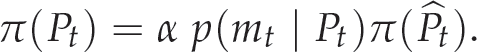
In the state estimation of a dynamic system, the vector P represents the state of the dynamic system. The measurement data available from the system output is m. The measurement data describes the action which is produced by the dynamic system by the control u. Bayes filters estimate the probability density function over the state space, conditionally to the measurements data and action produced by the system (control command). This probability is called the belief of the state vector and denoted as π(P_t).

π (P_{t}) = p (P_{t} | m_{0 \dots t}, u_{0 \dots t}) .

(5)

Without loss of generality, we assume that the measurements and the control commands arrive alternatively. In other words, the control command u_{t – 1} is the motion during the time interval [t – 1, t] while the current measurements at the time t is m_t. Based on the above assumptions, we can write the belief π(P_t) as

π (P_{t}) = p (P_{t} | m_{t}, u_{t - 1}, m_{t - 1}, u_{t - 2}, m_{t - 3}, \dots, m_{0}) .

(6)

The initial belief π(P₀) represents the initial knowledge about the system state. This initial knowledge is given by a probability function computed using the model of the system. This function is assumed to be uniform in the absence of an initial knowledge.

To derive the recursive update equation of the belief π(P_t), we use the Bayes rule, the Markov assumption, and we integrate over the state P_{t – 1} to write Equation (6) as

π (P_{t}) = α p (m_{t} | P_{t}) \int p (P_{t} | P_{t - 1}, u_{t - 1}) π (P_{t - 1}) d P_{t - 1},

(7)

where α is a normalizing constant [17].

The belief state π(P_t) is updated recursively at each iteration using the measurement data supplied at time t. Since the data, measurements and actions arrive alternatively, the algorithm can be divided into two stages: (1) prediction stage and (2) update stage. During the prediction stage, the system model (motion model) is used to get the a priori estimate of the state variable at time t using the famous Chapman-Kolomogorov equations [22]

π (\hat{P_{t}}) = \int p (P_{t} | P_{t - 1}, u_{t - 1}) π (P_{t - 1}) d P_{t - 1} .

(8)

The motion model p(P_t P_{t – 1}, u_{t – 1}) is defined as the state transition equation assuming the state is affected by a known Gaussian noise V_t – 1. The update stage consists of obtaining the measurements m_t and using it to update the a priori state estimate $π (\hat{P_{t}})$ . The posteriori density of the current state is given as

π (P_{t}) = α p (m_{t} | P_{t}) π (\hat{P_{t}}) .

(9)

The likelihood function p(m_t P_t) is defined by the system measurements. It is affected by known Gaussian noise n. One can note that the measurements play the key role in the update stage.

Therefore, starting from initial belief or a given knowledge about the system state, we have a recursive estimator of the state of the system that is partially observable. To implement Equation (7), we need to know the three distribution functions: the probability p(P_t P_{t – 1}, u_{t – 1}), the initial belief π(P₀), and the probability p(m_t P_t). The first one is the motion model of the system. The probability p(m_t P_t) is the sensor (measurement) model. One can note that the two models p(P_t P_{t – 1}, u_{t – 1}) and p(m_t P_t) are time invariant and they do not depend on the specific time t. We will see in the next section how particle filters can be used to implement the recursive update equation given in Equation (7).

The sequential importance resampling (SIR) algorithm is a popular particle filtering algorithm: this approximates the filtering distribution p(P_t m₀,…, m_t) by a weighted set of particles:

{(w_{k}^{(i)}, P_{t}^{(i)}) : i = 1, \dots, M} .

(10)

The importance weights w⁽ⁱ⁾_t are approximations of the relative posterior probabilities (or densities) of the particles such that $\sum_{i = 1}^{M} w_{t}^{(i)} = 1$ .

Since particle filters estimate an approximation of the state vector, it is very important to address the issue of its convergence with the true solution. More specifically, under what conditions is this convergence valid? An extensive treatment of the currently existing convergence results can be found in the excellent survey paper [23], where the authors consider stability, uniform convergence, central limit theorems and large deviations. The previously shown results prove the convergence of probability measures yet they only treat bounded functions, effectively excluding the most commonly used state estimate - the mean value. Later, in [24, 25], they prove the convergence of the particle filter for a somewhat general class of unbounded functions in the sense of L^P-convergence for an arbitrary p  2, applicable in many practical situations.

SIR filters with transition prior as importance function, are commonly known as ‘bootstrap filters’ or ‘condensation algorithms'. Other alternative varieties to particle filter are: Sequential importance sampling (SIS Gaussian particle filters, unscented particle filters, Monte Carlo particle filters and Gauss-Hermite particle filters. SIS is the same as SIR, but without the resampling stage.

3.3 Motion Model: Prediction Stage

Consider a world frame F₀ attached to the initial camera frame. This frame is considered fixed and all other frames will be defined with respect to it. Let the vector:

P = (\begin{matrix} t \\ q \end{matrix}) = (t_{X}, t_{Y}, t_{Z}, q_{1}, q_{2}, q_{3}, q_{4})^{T}

(11)

be the pose vector that represents the motion of the camera, where P is the pose vector of the camera frame related to a reference frame. In addition, let t = (t_X, t_Y, t_Z)^T be the translation vector and q = (q₁, q₂, q₃, q₄)^T be the rotation vector represented by the quaternion of the current camera frame. The translation and rotation are expressed in the initial camera frame, which is the world frame. One can note that the quaternion parametrization of the rotation requires a normalization step at each time iteration to ensure that it corresponds to the real rotation. A true rotation satisfies:

q_{1}^{2} + q_{2}^{2} + q_{3}^{2} + q_{4}^{2} = 1.

(12)

Let us recall from Eq (7) that our aim is to compute the posterior p(P_t m_t). The probabilistic transition state model p(P_t P_{t – 1}, u_{t – 1}) is considered such that the prediction equation is:

P_{t} = P_{t - 1} + Δ P_{t} .

(13)

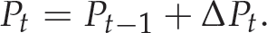
The quantity ΔP_t characterizes the motion model of the system. The smooth motion assumption is valid during the motion of the visual servoing system. Indeed, we choose the constant velocity model. This assumes that the camera travels at a constant velocity between any two time iterations or steps. In addition, the visual servoing controller produces a camera velocity at the current time step that is independent of the velocity at the previous time moment.

However, the velocity vector is still affected by noise and it needs to be augmented in order to set the state vector. Augmenting the velocity vector V = (v^T, w^T)^T with the pose vector, the state vector becomes:

P = {(\begin{matrix} t^{T} & q^{T} & v^{T} & w^{T} \end{matrix})}^{T} .

(14)

The change in the state vector is written as:

Δ P_{t} = {(\begin{matrix} Δ t v^{T} & Δ t Δ q^{T} & 0^{T} & 0^{T} \end{matrix})}^{T} .

(15)

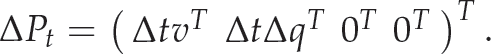
The vector Δ_q is a function of the Cartesian velocity computed by the visual servoing controller. To compute the vector Δ_q, we need to transform the changes in the rotation motion, i.e., the rotational velocity, from the Euler angles representation w^T = (w_x, w_y, w_z) to the quaternion representation $Δ q^{T} = ({\dot{q}}_{1}, {\dot{q}}_{2}, {\dot{q}}_{3}, {\dot{q}}_{4})$ . We can write Δq as follows:

Δ q = \frac{1}{2} W . q = \frac{1}{2} (\begin{matrix} 0 & - w_{x} & - w_{y} & - w_{z} \\ w_{x} & 0 & - w_{z} & w_{y} \\ w_{y} & w_{z} & 0 & - w_{x} \\ w_{z} & - w_{y} & w_{x} & 0 \end{matrix}) [\begin{matrix} q_{1} \\ q_{2} \\ q_{3} \\ q_{4} \end{matrix}],

(16)

where the matrix W is the transformation of the Euler rotation velocity parametrizations to the quaternion parametrizations.

The corruption of the velocity is modelled by the vector $n = (n_{v}^{T}, n_{w}^{T})$ , which is a zero mean Gaussian noise. Hence, the total motion model of the state vector is written as:

P_{t} = P_{t - 1} + Δ P_{t} + N .

(17)

P_{t} = P_{t - 1} + Δ P_{t} + (\begin{matrix} n_{v} Δ t \\ f (q, n_{w}) Δ t \\ n_{v} \\ n_{w} \end{matrix}),

(18)

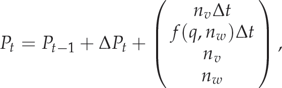
where f(q, n_w) is the noise affecting the rotational velocity represented using quaternion parametrizations. Note that we use in the prediction stage the a priori estimate of the velocity vector V given as the velocity signal produced by the visual controller.

3.4 Measurement Model: Update Stage

The measurement model considers the image points as image measurements. The measurement model is the epipolar constraint between two views. The essential matrix between two views can be written as a function of the rotation and translation between these two views as follows [15, 26]:

ℰ = [t]_{\times} R .

(19)

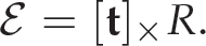
Since the camera is calibrated, the fundamental matrix ℱ is computed from the essential matrix ℰ using ℱ = 𝒦^−Tℰ𝒦⁻¹, which relates two image points, expressed in the pixel coordinates in the two views, as follows:

[u_{2}, v_{2},1] ℱ [u_{1}, v_{1} {,1]}^{T} = 0.

(20)

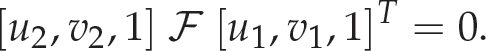
The above equation is called the ‘epipolar constraint’ between two images. The above equality holds only in cases where the fundamental matrix has been correctly computed. Geometrically, this equality means that the image point m₂ = [u₂, v₂, 1]^T in the second image belongs to the epipolar line:

l_{2} = ℱ m_{1} = ℱ {[u_{1}, v_{1},1]}^{T} .

(21)

This line l₂ corresponds to the image point m₁ = [u₁, v₁, 1]^T from the first image. The image measurement is considered correctly extracted up to this moment. Later, robustness techniques will be introduced to adapt to noisy image measurements. If we have an incorrect estimate of the fundamental matrix $\hat{ℱ}$ , the right-hand side of Equation (20) is not zero, and is denoted as:

d = m_{2}^{T} \hat{ℱ} m_{1} = d i s t^{2} (m_{2}, \hat{ℱ} m_{1}) .

(22)

Here, the value of this function h is the distance between the image point m₂ = [u₂, v₂, 1]^T and the epipolar line l₂ produced by substituting $\hat{ℱ}$ in equation (21) as it is shown in Fig 2.

The objective of the measurement model is to evaluate the hypotheses that represent the a priori motion distribution P_t+1/t. This distribution is computed using the Bayesian particle filter and the transition equation explained in the last subsection. The distribution is represented by M equally weighted particles $π (P_{t}) \approx {P_{t}^{i}, w_{t}^{i} = 1 / M}_{i = 1}^{M}$ These particles are evaluated using the epipolar constraints. Drawing M pose particles from the priority distribution given in (18) gives M a rigid transformation ${T^{i} = [R^{i}, t^{i}]}_{i = 1}^{M}$ . Here, the samples Rⁱ are computed from the quaternion vector q.

A set of M fundamental matrices ${ℱ}_{i = 1}^{M}$ , corresponding to the pose particles that represent the motion distribution, are computed using Equations (19). For a given image point $m_{1} = (u_{1}, v_{1} {,1)}^{T}$ in the first image, there are M epipolar lines ${l_{2}^{i}}_{i = 1}^{M}$ in the current image. Let us denote the distances ${h_{n}^{i}}_{i = 1}^{M}$ as the image distance between the image point $m_{2 n}$ and the epipolar line $l_{2 n}^{i}$ corresponding to the image point m_1n and the pose sample Pⁱ. Here, n = 1,…,N, where N is the number of image points.

The weight w^*(i) for each particle is computed as proportional to the following likelihood function:

w^{* (i)} \sim p (m | P^{i}) = \exp (D^{i} = - Σ_{n = 1}^{N} d_{n}^{i}),

(23)

where N is the number of the image features. The above measurement (likelihood) function is selected in the simplest form. It is the relationship between the image measurements and the epipolar line in the current view, corresponding to the image measurement in the initial view. The larger the summation $Σ_{n = 1}^{N} h_{n}^{i}$ , the further the pose sample is from the correct pose value. Indeed, the weight $w^{* (i)} \sim p (m | P^{i}) = \exp (D^{i} = - Σ_{n = 1}^{N} h_{n}^{i})$ is smaller. Similarly, if the summation is smaller then the pose sample is nearer, and the weight is larger.

Since the weight factors form a distribution, they need to be normalized. The normalized weights $w_{t}^{i}$ are given as:

w^{i} = w^{* (i)} / \sum_{i = 1}^{M} w^{* (i)} .

(24)

These weights $w_{t}^{* (i)}$ are the likelihoods of the samples Pⁱ with respect to the image measurement m. The resulting distribution ${P_{t}^{i}, w_{t}^{i}}_{i = 1}^{M}$ needs to be re-sampled to avoid the degenerate case. Details about resampling techniques can be found in [19]. The maximum likelihood sample is given as:

\bar{P} = \arg \max_{P^{i}} {p (m_{t} | P^{i})} .

(25)

The state vector, i.e., the pose vector P_{t t}, is updated at time t as the centre of gravity of the sample cloud, which is given as $P_{t | t} = \sum_{i = 1}^{M} w^{i} P^{i}$ . Some other methods that update the state vector by that sample that has the maximum likelihood or weight. This sample is precisely that given in Equation (25).

The geometrical representation of the particles of the pose vectors and the corresponding epipolar lines with respect to image point m₁ is given in Figure 2.

Figure 2.

Drawing M pose particles between the two views gives M epipolar lines which correspond to image point m₁. In the figure, the solid drawn epipolar line ${\hat{l}}_{2}$ - corresponding to image point m₁ and pose particle Pⁱ - is the nearest epipolar line with distance dⁱ to the image measurement m₂. Thus, the pose particle ${\hat{P}}^{i}$ is the most likely candidate to be the best estimate of the relative pose between the two views.

At each iteration, the estimated pose is used to estimate the 3D coordinates of the point features, as we have seen in Section 2 and particularly in Equation (2). The pose estimate along with the depth of features may be used in the position-based, image-based and hybrid visual servoing control laws. The use of the pose estimate and the depth estimate for visual servoing is discussed in the next section.

4. Model-free 3D Visual Servoing

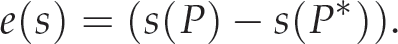
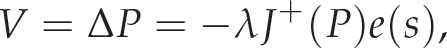
The camera pose alignment problem can be presented as a minimization problem of a suitable hybrid 2D/3D cost function. The positioning task is to move the robot end-effector from an initial pose P ∈ R³ × SO(3) to reach a desired pose P^*. In other words, the problem is to minimize an error vector e(s) of the visual features s(P) by finding a vector ΔP that minimizes a cost function E(s(P)). Viewing the problem as a nonlinear least squares minimization problem allows us to formulate the following cost function:

E (s (P)) = \frac{1}{2} e {(s)}^{T} e (s) .

(26)

where:

e (s) = (s (P) - s (P^{*})) .

(27)

To minimize the cost function, Gauss-Newton minimization is used. The required change in the pose is thus:

V = Δ P = - λ J^{+} (P) e (s),

(28)

where $\frac{\partial E (s (P))}{\partial P} = J (P)$ and the matrix

J^{+} (P) = ((J^{T} (P) J (P {))}^{- 1} J^{T} (P)

is the pseudo-inverse of the matrix J. This method is widely used in robot control and visual servoing [27,28].

3D visual features, such as position and orientation, can be part of the feature vector S_3D(P) = [T_x, T_y, T_z, uθ]^T. Here, the notion uθ is the Euler axis/angle parametrization [15] of the rotation. The desired features are S_3D(P^*) = [T^*, uθ]^T. Hence, we can write:

E_{3 D} (s (P)) = \frac{1}{2} e_{p} {(P)}^{T} e_{p} (P),

(29)

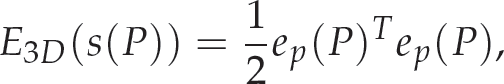
where:

e_{p} (P) = s_{3 D} (P) - s_{3 D} (P^{*}) .

(30)

Let us select the vector of 3D features as $s_{3 D} (P {) = [}^{C^{0}} T_{C},^{C^{0}} {(u θ)}_{C}]^{T}$ , i.e., the relative pose between the current camera frame F_C and the initial one F_C0. The desired features can be set here as $s_{3 D} (P^{*} {) = [}^{C^{0}} T_{C^{*}},^{C^{0}} {(u θ)}_{C^{*}}]^{T}$ , i.e., the relative pose between the desired camera frame F_C* and the initial one $F_{C^{0}}$ . The set of desired features S_3D(P^*) can be computed once in advance of the servoing process as an offline step. Decomposing the homography or the essential matrix [15, 29] produces an estimate of the scaled translation $^{C^{0}} T_{C^{*}}$ and the rotation $^{C^{0}} {(u θ)}_{C^{*}}$ . One might note that this selection of features, i.e., a 3D pose vector within PBVS, does not require the 3D model of the target object.

We use the pose estimation algorithm presented in the previous section to estimate the camera motion between the initial and current images. This relative pose is nothing but the feature vector S_3D^(P). The a priori camera motion distribution is computed using the velocity control signal sent by the visual controller to the robot joint controller.

The Cartesian Jacobian J_p(P) is given in this case by:

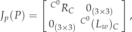
J_{p} (P) = [\begin{matrix} ^{C^{0}} R_{C} & 0_{(3 \times 3)} \\ 0_{(3 \times 3)} & ^{C^{0}} {(L_{w})}_{C} \end{matrix}],

(31)

while the error function is:

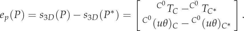
e_{p} (P) = s_{3 D} (P) - s_{3 D} (P^{*}) = [\begin{matrix} ^{C^{0}} T_{C} -^{C^{0}} T_{C^{*}} \\ ^{C^{0}} {(u θ)}_{C} -^{C^{0}} {(u θ)}_{C^{*}} \end{matrix}] .

(32)

One might note that the 3D feature used for this position-based visual servoing are different from previous algorithms that have appeared in the literature. We use the relative pose between the current and the initial camera frames, while earlier algorithms use the relative pose between the current and the target camera frames. Figure 3(a) illustrates the 3D feature S_3D(P) used in our algorithm, while the earlier feature vector is shown in Figure 3(b). This new choice of features is justified, since our proposed pose estimation algorithm estimates the relative pose between the initial and current camera poses. In fact, the pose estimation algorithm accumulates the velocities and recursively corrects them at every time instance using the particle filter.

Figure 3.

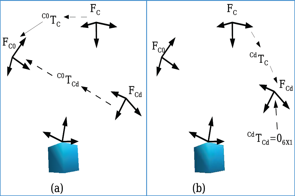
The current and desired 3D feature vectors: (a) our model-free method, $s_{3 D} (P {) = [}^{C^{0}} T_{C},^{C^{0}} {(u θ)}_{C}]^{T}$ , and (b) the classical model-based method, $s_{3 D} (P {) = [}^{C^{*}} T_{C},^{C^{*}} {(u θ)}_{C}]^{T}$

5. Experimental Results

In this section, we present the results from two experiments. First, we present the results from testing our algorithm regarding pose estimation for a specific controlled motion. Then, another experiment is carried out using the position-based visual servoing algorithm presented in this paper that utilizes our proposed pose estimation algorithm. The task here is pure rotation about the camera optical axis. This is one of the most challenging tasks in the visual servoing literature [30].

5.1 Results for Pose Estimation

The algorithm is tested using the real robot setup available at the Robotic Intelligence Lab of Jaume-I University, Spain. The robot is a PA-10 7-DOF manipulator arm manufactured by Mitsubishi. An external view of the setup is shown in Figure 6. A single IEEE-1394 camera is attached to the end-effector. The camera has been calibrated by imaging a planar calibration grid from 20 viewpoints over the hemisphere and using the camera calibration toolbox for MATLAB [31] to compute the intrinsic and extrinsic parameters. Image processing and robot control are performed by the ViSP library [32], while the particle filter is implemented with the Bayesian Filtering Library [33].

The target consists of four white circles of 1 cm radius over a black background arranged in a square with 15 cm sides. The feature points are computed as the first-order moments (centroids) of the segmented circles. It has been shown that the Jacobian matrix related to such coordinates is a generalization of the Jacobian matrix related to the coordinates of a point [34]. Such an approximation is not a problem since robustness with respect to modelling errors is a well-known feature of closed-loop visual servoing.

In this experiment, the robot runs a specific controlled motion task. The task consists of a considerable amount of translation and rotation. It is complex enough to show the efficiency of the filter in estimating rotational and translational motion as well as the scale of the translational motion. The algorithm runs independently to estimate the actual motion of the arm. We measured the time elapsed from frame acquisition to the filter update during the experiment. This time is measured in microseconds, averaging slightly less than 70 ms; thus, the frame rate is about 15 frame / second (fps). Methods that use VVS for pose estimation, like [12, 35, 36], have reported the same frame rate of 15 fps. The filter prediction and update stages take approximately 35 ms. The remaining time is spent for feature extraction and image acquisition. This time is slightly less than that reported in [9] for the EKF, i.e., 36 ms, but much less than the iterative extended Kalman filter (IEKF) and the IAEKF, i.e., 62 ms and 78 ms, respectively. However, it was reported in [9] that the IEKF and the IAEKF produce a similar error to ours, i.e., within scale of one millimetre and 0.01 radians; meanwhile, the error produced by the EKF is much larger, i.e., within a scale of 10 millimetres and 0.1 radians.

Figure 4 shows a comparison of the actual motion of the robot measured by the joint angles with the robot motion estimated using our particle filter algorithm. The plots in column (a) show the motion measured by the robot joints. Column (b) represents the motion which is estimated by the filter. Column (c) shows the difference error between the robot motion measured by the robot joints and the motion estimated by the proposed filter. Column (d) shows the motion produced by simply accumulating the velocity signal produced by the visual controller without correction. The translational motion is in the upper row while the rotational motion is in the lower row. The plots in (c) show a small amount of error between the actual measured robot motion and the estimated motion using the filter. Figure 5 shows the camera movement in the 3D space for the robot motion, the filter estimate and the accumulated velocity.

Figure 4.

Comparison of the actual robot motion with the estimated robot motion using the particle filter during a specific motion command given to the robot testing the pose estimation accuracy. The translational motion is at the top while the rotational motion is at the bottom. The plots in column (a) show the motion measured by the robot joints. Column (b) represents the filter estimate of the motion. Column (c) shows the difference between the robot motion estimated by the robot joints and the motion estimated by the proposed filter. The small error shown in (c) reflects the accuracy of the filter. Finally, column (d) shows the motion resulting by the accumulation of the velocity signal alone. One can clearly see here that the considerable amount of drift motion added by the arm joints with respect to the velocity control signal is corrected by the filter.

Figure 5.

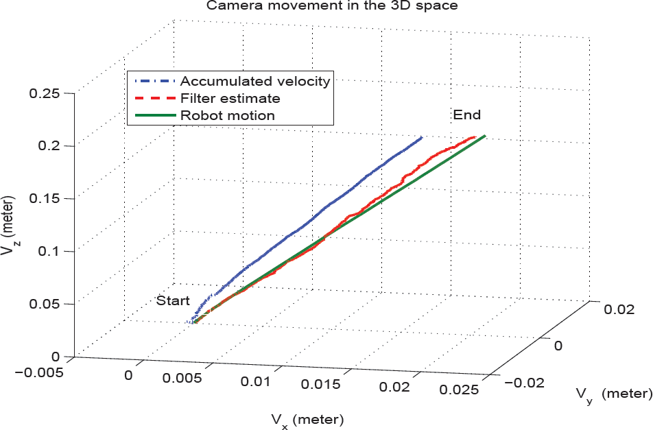
The camera motion in the 3D space

Figure 6.

External view of the experimental setup

Looking at the results reported in Figure 4, one can see that the error is bounded within an acceptable range. The error in the linear motion is on average about 1-2 millimetres. In addition, one can see the difference between the commanded motion, i.e., the accumulated velocity signal in (d) and the actual motion measured by the robot joints. The amount of rotational motion produced by accumulating the velocity signal is almost −0.47 radians. In contrast, the amount of rotational motion estimated by the filter is −0.55 radians. This gives a result with an error of 0.08 radians drift motion by the robot, while the error in rotational motion between the filter estimate and actual robot motion is 0.015 radians. One can clearly see here that the considerable amount of drift motion added by the arm joints with respect to the velocity control signal is corrected by the filter. This proves the efficiency of the proposed filter.

One more thing to note from the figures is that the error in translational motion is relatively less erroneous than for the rotational motion. This is the reason why we focus on rotational motion in the next experiment, i.e., 3D visuals based on the proposed pose estimation method. In the next subsection, a visual servoing experiment is presented. The selected task is pure rotation around the optical axis, since it is perceived to be the most critical task in the visual servoing literature [30].

5.2 Results from Visual Servoing

As we have shown earlier in this paper, the objective of this work is to estimate, in real-time, the 3D parameters (here, the camera pose) to be used by the visual servoing algorithm. In the following, we present a model-free visual servoing example using the pose estimation algorithm which was presented in this paper.

The proposed task is one of the most challenging in visual servoing, i.e., a rotation of 90° about the camera's optical axis. The servoing process aims to minimize the error between the initial current camera pose and the initial desired camera pose. The proposed visual servoing control law computes this pose error and then produces a velocity control signal proportional to this error. This error is equal to the relative pose between the initial and desired views at the initial time. This pose is partially estimated using the homography matrix, which decomposed to obtain the rotation ^*R₀ and the scaled translation ^*t₀ between the two initial and desired views.

The role of our pose estimation algorithm is to compute the actual motion of the arm. This is the relative pose between the initial and current views. This is represented by the rotation ⁱR₀ and the translation ⁱt₀. This computed motion is used as the feature to control the robot motion as indicated by the error function shown in Equation (32) and Figure 3(a). One can note from Equation (32) that the scale of translation in PBVS is not critical, since we are interested in the direction of translation only, while the scale of it is controlled by the remaining current error e_p(P) = S_3D(^P) – S_3D(^P*). Hence, estimating the desired initial camera pose up to the scaled translation is sufficient to start the servoing process, hence moving the arm in the proper direction.

The selected servoing task is one of the most challenging tasks in visual servoing, i.e., a rotation of 90° about the camera's optical axis. Based on the control law designed in section 4, the performed motion should be pure rotation about the Z axis, i.e., the camera's optical axis with a zero translation vector. The results from this visual servoing experiment are depicted in Figure 7 and Figure 8. The image trajectory of the features is shown in Figure 7(a). The desired position of the features is marked by ‘+'. The velocity signal is shown in Figure 7(b). The linear velocity is at the top while the rotational velocity is at the bottom. The linear velocity control signal is null and is produced by zero estimated translation, which is identical to the real case. This proves the efficiency of the filter. Similarly, the rotational motion is pure rotation about the camera's optical axis. This reflects the fact that both the rotation and translation estimation processes are efficient.

Figure 7.

Trajectories in the image space in (a) and the screw velocity in (b) of the vision control algorithm based on the epipolar pose estimation algorithm. The task is 90° rotation about the optical camera axis. The linear velocity control signal is null and is produced by zero estimated translation, which is identical to the real case. This proves the efficiency of the filter. Similarly, the rotation motion is pure rotation about the camera's optical axis. This reflects the fact that both the rotation and translation estimation processes are efficient.

Figure 8.

Comparison of the actual robot motion with the estimated motion using a particle filter and the accumulated velocity during the visual servoing task to show the accuracy of the pose estimation algorithm using our proposed filter. The plots in column (a) show the motion measured by the robot joints. Column (b) represents the filter estimate of the motion. Column (c) shows the difference between the robot motion estimated by the robot joints and the motion estimated by the proposed filter. The small error shown in (c) reflects the accuracy of the filter. Finally, column (d) shows the motion resulting from accumulating the velocity signal alone. One can clearly see here that the considerable amount of drift motion added by the arm joints with respect to the velocity control signal is corrected by the filter.

The motion which is performed by the above visual servoing task is depicted in Figure 8. The actual robot motion measured by its joints in Figure 8(a) is compared with the motion estimated by the filter in Figure 8(b). The translation motion should be null, since the task is pure rotation. Due to the error in the filter estimate, we can see very small amounts of translational motion, but this motion is small and insignificant. The error between the filter estimate and the actual robot motion is shown in Figure 8(c). In addition, the motion – which is produced by simply accumulating the velocity – is shown in Figure 8(d). A considerable amount of drift motion by the robot can be seen by comparing (a) with (d). The commanded motion is almost −0.9 radians while the robot has performed −1.57 radians, with a total drift motion of 0.67 radians. However, the filter is efficiently able to estimate the motion with an error bounded by 0.05 radians (a factor of 10).

The convergence of the visual servoing process as indicated in Figure 7 and the error in the filter pose estimate in Figure 8 prove the accuracy of the pose estimation results. Once again, let us note here that a considerable amount of drift motion added by the arm joints with respect to the velocity control signal is corrected by the filter.

6. Conclusions

This paper presents a probabilistic method for the estimation of the current camera pose with respect to its initial pose. The method uses a particle filter to estimate the relative pose of the camera between the initial and the current frames, while a two-view geometry is used to estimate and reconstruct the 3D model of the environment or the target object. Unlike previous probabilistic methods, this work uses a priori knowledge about the motion to include the amount of translation in the state vector. This is useful in making the method suitable for real-time applications, like visual servoing. Consequently, model-free visual servoing can be performed for image-based, position-based or hybrid visual servoing.

7. Acknowledgements

This paper describes research done at the Robotic Intelligence Laboratory. Support for this laboratory is provided in part by Ministerio de Economia y Competitividad (DPI2011–27846), by Generalitat Valenciana (PROMETEOII/2014/028) and by Universitat Jaume I (P1-1B2011-54).

References

Chaumette

and Hutchinson

. Visual servo control, part I: Basic approaches. IEEE Robotics and Automation Magazine, 13(4):82–90, December 2006.

Hafez

A.H. Abdul

and Jawahar

C.V.

. Visual servoing by optimization of a 2D/3D hybrid objective function. In IEEE Int. Conf. on Robotics and Automation, ICRA'07, Roma, Italia, April 2007.

Hafez

A.H. Abdul

Cervera

, and Jawahar

C.V.

. Optimizing image and camera trajectory using on-line boosting. In IEEE/RSJ Int. Conf. on Intelligent Robots and Systems, IROS'07, San Diego, CA, October 2007.

Penate-Sanchez

Andrade-Cetto

, and Moreno-Noguer

. Exhaustive linearization for robust camera pose and focal length estimation. IEEE Transactions on Pattern Analysis and Machine Intelligence, PAMI, 35(10):2387–2400, 2013.

Do-Hwan

Jeong-Hoon

, and In-Joong

. Novel position-based visual servoing approach to robust global stability under field-of-view constraint. IEEE Transactions on Industrial Electronics, 59(12):4735–4752, 2012.

Tahri

Araujo

Mezouar

, and Chaumette

. Efficient decoupled pose estimation from a set of points. In IEEE/RSJ Int. Conf. on Intelligent Robots and Systems, IROS'2013, Tokyo, Japan, November 2013.

Deng

Wilson

W.J.

, and Janabi-Sharifi

. Decoupled EKF for simultaneous target model and relative pose estimation using feature points. In 2005 IEEE Conference on Control Applications, pages 749–754, Toronto, Canada, August 2005.

Chen

S.Y.

. Kalman filter for robot vision: A survey. IEEE Transactions on Industrial Electronics, 59(11):4409–4420, 2012.

Janabi-Sharifi

and Marey

. A Kalman-filter-based method for pose estimation in visual servoing. IEEE Trans. on Robotics, 26(5):939–947, October 2010.

10.

Tahri

and Chaumette

. Complex objects pose estimation based on image moment invariants. In IEEE Int. Conf. on Robotics and Automation, ICRA'05, pages 438–443, Barcelona, Spain, April 2005.

11.

Marchand

and Chaumette

. Virtual visual servoing: a framework for real-time augmented reality. Computer Graphics Forum, 21(3):289–298, September 2002.

12.

Gratal

Bohg

Romero

, and Kragic

. Visual servoing on unknown objects. Mechatronics, 22(4):423–435, 2012.

13.

Forsyth

D.A.

Haddon

, and Ioffe

. The joy of sampling. International Journal of Computer Vision, 41(1 and 2):109134, 2001.

14.

Qian

and Chellappa

. Structure from motion using sequential Monte Carlo methods. International Journal of Computer Vision, 59(1):5–31, 2004.

15.

Hartley

and Zisserman

. Multiple View Geometry in Computer Vision. Cambridge University Press, second edition, 2003.

16.

Pupilli

and Calway

. Real-time camera tracking using a particle filter. In British Machine Vision Conference, BMVC'05, pages 519–528, Oxford, September 2005.

17.

Thrun

Burgard

, and Fox

. Probabilistic Robotics. The MIT Press, 2005.

18.

Doucet

. On sequential simulation-based methods for Bayesian filtering. Technical Report CUED/F-INFENG/TR. 310, Cambridge University Department of Engineering, 1998.

19.

Arulampalam

Maskell

Gordon

, and Clapp

. A tutorial on particle filters for on-line non-linear/non-Gaussian Bayesian tracking. IEEE Transactions on Signal Processing, 50(2):174–188, February 2002.

20.

Kalman

R.E.

and Schiele

. A new approach to linear filtering and prediction problems. Transactions of the ASME – Journal of Basic Engineering, 82:35–45, 1960.

21.

Vihola

. Random Sets for Multitarget Tracking and Data Fusion. PhD thesis, Tampere University of Technology, Tampere, 2004.

22.

Papoulis

. Probability, Random Variables and Stochastic Processes. McGraw-Hill series in electrical engineering, New York, 2nd edition, 1984.

23.

Crisan

and Doucet

. A survey of convergence results on particle filtering methods for practitioners. IEEE Transactions on Signal Processing, 50(3):736âĂŞ–746, 2002.

24.

X.-L.

Schön

T. B.

, and Ljung

. A general convergence result for particle filtering. IEEE Transactions on Signal Processing, 59(7):3424–3429, July 2011.

25.

X.-L.

Schön

T. B.

, and Ljung

. A basic convergence result for particle filtering. IEEE Transactions on Signal Processing, 56(4):1337–1348, April 2008.

26.

Faugeras

. Three-Dimensional Computer Vision: A Geometric View point. MIT Press, Cambridge, MA, USA, 1993.

27.

Espiau

Chaumette

, and Rives

. A new approach to visual servoing in robotics. IEEE Trans. on Robotics and Automation, 8(3):313–326, June 1992.

28.

Malis

. Improving vision-based control using efficient second-order minimization techniques. In IEEE Int. Conf. on Robotics and Automation, ICRA'04, New Orleans, USA, April 2004.

29.

Malis

Chaumette

, and Boudet

. 21/2 D visual servoing. IEEE Transactions on Robotics and Automation, 15(2):238–250, April 1999.

30.

Chaumette

. Potential problems of stability and convergence in image-based and position-based visual servoing. In Kriegman

Hager

, and Morse

A.S.

, editors, The Confluence of Vision and Control, pages 66–78. LNCIS Series, No 237, Springer-Verlag, 1998.

31.

Bouguet

J.Y.

. Camera calibration toolbox for MATLAB, 2008.

32.

Marchand

Spindler

, and Chaumette

. Visp for visual servoing: a generic software platform with a wide class of robot control skills. IEEE Robotics and Automation Magazine, 12(4):40–52, December 2005.

33.

Gadeyne

. BFL: Bayesian Filtering Library. http://www.orocos.org/bfl, 2001.

34.

Chaumette

. Image moments: a general and useful set of features for visual servoing. IEEE Trans. on Robotics, 20(4):713–723, August 2004.

35.

Gratal

Romero

, and Kragic

. Virtual visual servoing for real-time robot pose estimation. In 18th IFAC World Congress, Milano, Italy, August 2011.

36.

Comport

A.I.

Marchand

Pressigout

, and Chaumette

. Real-time markerless tracking for augmented reality: the virtual visual servoing framework. IEEE Trans. on Visualization and Computer Graphics, 12(4), July 2006.

Particle-filter-based Pose Estimation from Controlled Motion with Application to Visual Servoing

Abstract

Keywords

1. Introduction

2. Background of Multiple View Geometry

3.1 Overview of the Proposed Method

5.1 Results for Pose Estimation

7. Acknowledgements

References