Sage Journals: Discover world-class research

Abstract

The paper compares the performance of several methods used for the estimation of an image Jacobian matrix in uncalibrated model-free visual servoing. This was achieved for an eye-in-hand configuration with small-amplitude movements with several sets of system parameters. The tested methods included the Broyden algorithm, Kalman and particle filters as well as the recently proposed population-based algorithm. The algorithms were tested in a simulation environment (Peter Corke's Robotic Toolbox for MATLAB) on a PUMA 560 robot. Several application scenarios were considered, including static point and dynamic trajectory tracking, with several characteristic shapes and three different speeds. Based on the obtained results, conclusions were drawn about the strengths and weaknesses of each method both for a particular setup and in general. Algorithm-switching was introduced and explored, since it might be expected to improve overall robot tracking performance with respect to the desired trajectory. Finally, possible future research directions are suggested.

Keywords

Visual Servoing Model-free Uncalibrated Population-based Particle Filter

1. Introduction

The use of visual sensors in robot control loops has been discussed in the literature (and in practice) for a number of years [1, 2], since computer vision sensors provide information-rich signals which are very useful, especially in unknown environments [3 –7]. This paper focuses on an image-based visual servoing (IBVS) approach in which control error is defined in the image plane, enabling the use of an uncalibrated and model-free approach [8, 9]. To achieve this, a Jacobian matrix needs to be calculated/estimated to define dependencies between changes in the camera coordinate frame (visual changes) with changes in the robot coordinate frame (robot angle changes). Since the early 2000s, several approaches to image matrix estimation have emerged based on nonlinear optimization algorithms [8 –12] which are a significant improvement on traditional methods for Jacobian estimation.

The large body of work produced and the numerous available methods might suggest that the problem of visual servoing is trivial, but the implementation of the specific setup/problem reveals drawbacks (and advantages) with each individual method. There appears, however, to be no significant research comparing uncalibrated model-free image-based visual servoing methods (especially for small-amplitude movements). Additionally, the question of the integration of several estimation methods is still very much open. Thus, this paper tries to present the specific characteristics of several methods applied in a simulation problem: the positioning of an object in a specified position in space, and the identifying of scenarios in which the methods provide the best results. This was achieved for an eye-in-hand configuration [13] with a PUMA 560 robot manipulator for the small-amplitude movements that are characteristic of high-precision tasks, something which has not been widely studied in the literature. The contributions of the manuscript can be summarized as follows:

–

A comparison and analysis of the performance of widely-used methods applied in uncalibrated and model-free IBVS on several characteristic trajectories (both static and dynamic) for small-amplitude movements.

–

The application and analysis of population- and particle filter-based visual servoing for an eye-in-hand configuration (sparsely represented in the literature).

–

The application of the Kolmogorov-Smirnov statistical test for the analysis of similarities between end-effector trajectories.

–

The discussion of the real-time integration of several IBVS algorithm outputs for the best adaptation of the control system to the environment.

The article is structured as follows. Section 2 contains a brief literature review which highlights the current state of the art and identifies possible room for improvement. Section 3 presents the experimental design used for simulation, and introduces the reader to the image Jacobian matrix and the estimation algorithms used. The results are presented and discussed in Section 4 with respect to the evaluation parameters introduced in Section 3. Finally, Section 5 concludes and suggests possible future research directions.

2. Image-based visual servoing – A brief literature review

Visual servoing for robots has received significant attention since the late-1990s [7], and so the available literature on the subject is significant and goes well beyond the scope of this paper. The research field can be divided according to two main categories [14 –17]: PBVS (position-based visual servoing, also known as 3D visual servoing), and IBVS (also known as 2D visual servoing). It should be noted that a third (hybrid) approach also exists which is a combination of these two approaches [18]. A comparison of PBVS and IBVS methods is provided in [17]. The authors were concerned with three fundamental characteristics of two approaches to visual servoing: stability, robustness and sensitivity. It was shown that both approaches are locally asymptotically stable with no modelling errors, and are locally robust to such errors. However, they could not handle large motion commands. Trajectories as well as convergence rates were affected by all types of error. With regard to sensitivity, the two approaches showed the same trends, depending upon the type of reference.

Because of the advantages which IBVS offers, such as definition of control error in terms of image features and robustness to system modelling and image measurement errors [14, 19–24], it is an interesting robot control tool. IBVS includes a special subset where no camera calibration or knowledge of an exact system model (e.g., model-free) is needed, and it offers additional flexibility, especially in unknown and unstructured environments [8, 9]. An additional division can be made based on the procedure used for the calculation of an image Jacobian [9, 17]. This type of visual servoing problem could be formulated as a nonlinear least squares problem in which the goal function (error) needs to be minimized. The first application of image Jacobian estimation was proposed in Hosoda et al. [4], where a model-free but calibrated approach was adopted. One of the first efficient solutions for a model-free approach was offered by Jägersand et al. [5], who formulated the visual servoing problem as a nonlinear least squares problem solved by a quasi-Newton method with Broyden Jacobian estimation. Stability was ensured by the thrust region method. Similar principles have also been applied for multiple camera model-based 3D visual servoing [6]. If the target is moving, the error is not only a function of the robot poses but also of the poses of the moving object. Consequently, Piepmeier [12, 20] suggested the use of a dynamic quasi-Newton uncalibrated model-free method with a recursive estimation scheme for Jacobian calculation. This estimation actually involved integrated velocity prediction and correction. The velocity prediction and correction term was calculated as the time derivate of target motion which attempted to compensate for target motion, in turn resulting in better tracking performance. Testing of the proposed method was done with a 6DOF PUMA robot.

Recently, the generalized secant method has been suggested [8] as best fitting the model of a nonlinear system. The method stores data from a certain number of data points in the past and uses them in future decision-making, which has favourable effects on overall visual servoing performance. Hao and Sun in [9] proposed a universal state space approach after examining several approaches to the estimation of an image Jacobian, including a population-based method. This was motivated by the desire to address the sensitivity to noise and error of the Broyden approach. They argue that their universal state space approach provides a standardized framework into which all approaches to uncalibrated model-free visual servoing can be fed, and that it provides a framework for the identification of connections between different approaches. It is interesting to note that they conclude that a variant of the population-based method with 20 members obtained the best results for dynamical tracking. This work is close to the subject of our study, but since the authors were primarily concerned with a unified state space framework, performance comparison is not fully explored, especially for small-amplitude movements. Thus, our work expands on that of [9].

Another class of methods relies on estimators like (extended) Kalman and particle filters for the estimation of elements in an image Jacobian matrix [25, 26]. The advantage of this kind of approach (besides the computational efficiency of Kalman filters and the power of particle filters) is the existence of a covariance matrix which provides the algorithm with confidence in its estimate, thus enabling the inclusion of innovative data-fusion approaches to visual servoing. Kalman filters can also be used for the estimation of object motion in an image, thus improving tracking accuracy [27, 28]. One known issue with Kalman filters is the need for knowledge of process and measurement noise, which are in general not known or constant. Thus, an adaptive Kalman filter [27, 28] is employed which tries to adapt these statistics in order to maximize estimation accuracy. Another way to improve the performance of a Kalman filter is to use motion-primitive models [29] and a strategy for switching between them using validation gates implemented by nonlinear least square fitting. In the particular paper, only two primitives were used – linear and circular motion – but the authors stress that this was enough to construct complex trajectories. They go on to state that additional primitive models can easily be added.

Since these methods update the image Jacobian matrix according to changes in image features, the question arises as to how the initial matrix is estimated. This is done with exploratory movements [6], whereby the robot is moved by very small and known increments (joint-by-joint; all other joints are kept constant in the particular case). On the basis of the recorded changes in image features, the initial Jacobian matrix is calculated. The stability of the estimation method has been proved [4, 11] to depend significantly on the accurate estimation of this initial matrix. When choosing image features to track, one should bear in mind possible instability because of the singularity of the Jacobian matrix, as shown in [30 –32]. This is the reason why the desired and target shapes in [12, 19] do not fully match. Sutanto et al. [6] originally examined deterioration in an image Jacobian matrix due to the assumption of a constant matrix for N robot movements (because of a reduction in computational demands). This situation is especially pronounced when several consecutive joints are moved in the same direction (which is a common occurrence). Sometimes, it is also necessary to take into account the specifics of applied hardware, as was the case in [14] where epipolar constraints or/and a fundamental matrix were taken into account (for stereovision), thus increasing the robustness of the method. This was verified on a 3DOF system.

The literature review reveals that there is no significant research on uncalibrated model-free image-based visual servoing methods (an exception is [9]) for small-amplitude movements which compares traditional approaches with some rarely-used or novel approaches. Additionally, the question of the possible integration of several methods to provide more reliable and accurate estimates is still very much open.

3. Materials and methods

3.1. Experimental setup

In the simulation study, a 6DOF Puma 560 industrial robot was used for the experiments. This was achieved with the Robotics and Machine Vision Toolbox for MATLAB created by Peter Corke [33]. This toolbox is widely recognized in the visual servoing community and has been used in a number of previous papers [9, 12, 20, 32]. An eye-in-hand configuration was used in such a way that the manipulator end-gripper and camera coordinate frames coincided. In this way, processing was simplified and generality of discussion maintained. Figure 1 depicts an example of the robot setup and its pose during simulation, as well as current and desired image feature positions.

Figure 1.

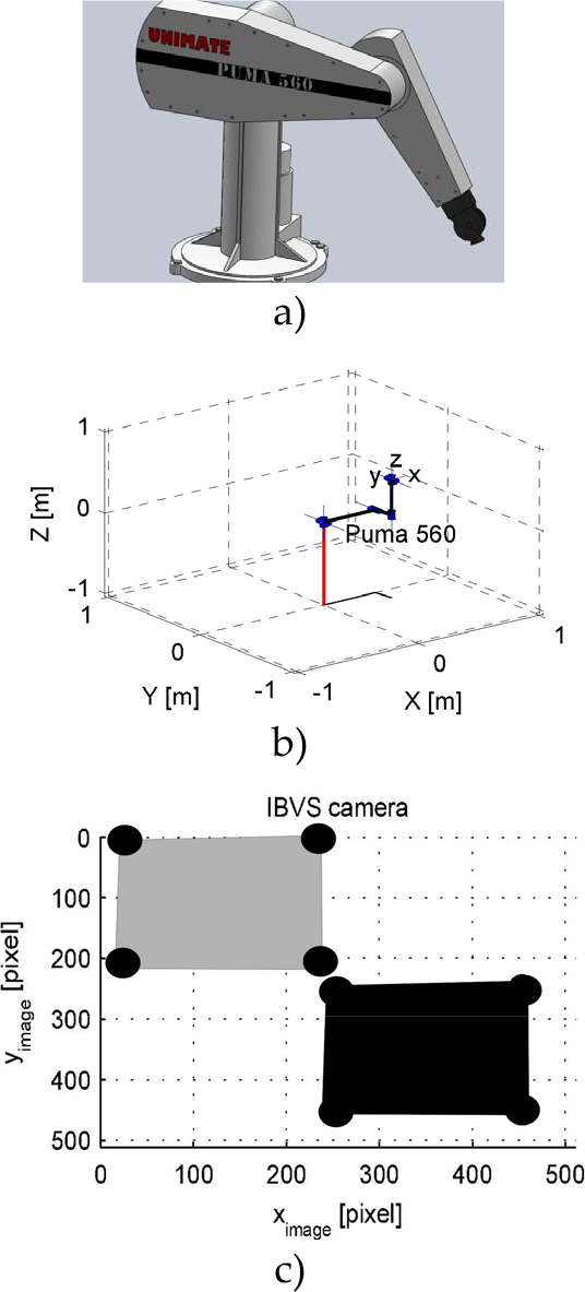
Simulation setup: a) 3D view of the robot, b) 6DOF Puma 560 robot manipulator in the simulation environment, c) view from the eye-in-hand camera comparing the current pose (black) and the desired pose (grey).

From Figure 1c, it can be seen that four points on the end-effector (i.e., image features) do not constitute a rectangle because of possible singularity issues, as suggested in [25, 30, 31]. The target was positioned (and moved) mainly in the Y-Z plane, as defined in Figure 1b. The camera parameters were set to the following values: image plane size 512×512 pixels, focus length f = 8 mm and pixel projection ratio P = 60 pixel/mm. The camera sampling time was set to 0.02 s, and visual servoing algorithms and a simulation were run with a 0.01 s sampling time. Thus, rate transition blocks were inserted before (zero-order hold) and after (unit delay) the camera.

Two types of scenarios were explored: static target-tracking and dynamic target-tracking. In both cases, zero mean Gaussian noise was added with variances of σ² = 0 (i.e., no noise), σ² = 0.5 and σ² = 1. Noise was added to the measurement of the image features. The static case demonstrated the algorithm's convergence and steady-state performance parameters. In the dynamic case, three characteristic trajectories were chosen (a diagonal line, a rectangle and a circle) in order to test the algorithm's tracking capabilities, robustness in terms of prediction bias and performance subject to abrupt changes. The influence of the target speed was also analysed, and thus each trajectory was simulated at three speeds (in the image plane): 10 pixels/s, 20 pixels/s and 30 pixels/s. Additionally, in every case performance was tested with and without velocity prediction and correction. Four online image Jacobian matrix estimators were used (the Broyden method, a Kalman filter, a particle filter and a population-based method) along with the analytical calculation of the matrix as the reference. Thus, in total 5×3×2 (static case: number of methods, noise levels, velocity prediction and correction) + 5×3×3×2 (dynamic case: number of methods, target speed levels, number of noise levels, velocity prediction and correction) = 120 simulation runs were performed in this study.

The initial image Jacobian matrix estimation was based on [6], where small, exploratory movements of each individual robot joint (while other joints were kept constant) were made. In this manner, the correspondence between each joint displacement and the displacement of image features was established. This step needs to be executed carefully, since errors can make visual servoing – regardless of the method used – unstable. Since the Puma 560 has six joints, six exploratory steps were executed, each providing two elements (one for the x axis and one for the y axis) of the Jacobian matrix. This can be written formally for a single image feature as:

J_{0} = [\begin{matrix} \frac{Δ x_{1}}{Δ θ_{1}} & \dots & \frac{Δ x_{6}}{Δ θ_{6}} \\ \frac{Δ y_{1}}{Δ θ_{1}} & \dots & \frac{Δ y_{6}}{Δ θ_{6}} \end{matrix}]

(1)

where $∆ x_{i}$ and $∆ y_{i}$ denotes changes in the x and y values (respectively) of the image feature when the joint i is moved for the angle $∆ θ_{i}$ while all other joint angles are kept at a constant initial value.

3.2. Image Jacobian estimation algorithms

The general principle of IBVS control is depicted in Figure 2, although in the study itself joint angular velocities rather than joint angles were used for control. As can be seen from the figure, the visual servo controller takes as inputs the differences in image features and robot joint angles between two consecutive time instances and, according to a predefined optimization/estimation algorithm, provides an image Jacobian matrix. Please note that some image processing algorithms are needed (e.g., feature-tracking algorithms like the Lucas-Kanade algorithm [34]) to obtain the image feature vector. The Jacobian matrix is used to define changes in the joint angles' values necessary to minimize the residual error function (i.e., to get closer to the desired target). For the eye-in-hand configuration, the residual error function is defined as:

Figure 2.

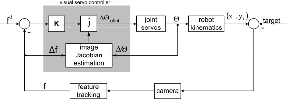
A general IBVS control scheme, where: f^d denotes the desired image feature values, f denotes the current image feature values, Δf denotes the change in image feature values between two consecutive frames, ∆θ_robot denotes the required change in robot angle values, θ denotes the current robot angle value's vector, ∆θ denotes the actual change in robot angle values between two consecutive time instances, and (x_i, y_i) are the coordinates of respective robot joints in the world coordinate frame.

f (θ, t) = {f_{d e s i r e d} - f}_{a c t u a l} (θ, t)

(2)

A robot kinematics block was used to reconstruct the x and y coordinates of each individual joint/segment based on the robot joint angles. In the simulation study, forward kinematics was used as depicted in Figure 3 (which was later adapted to include rate transition blocks). In practice, this block is not needed (except in cases where analytical calculation of the image Jacobian is performed). It was used to simulate the real robot movement, something which is readily available in practical applications. Also, please note the integrator in the loop for the transition from speed control to position control. In the study, a proportional controller was used, such that the control signal could be defined as:

Figure 3.

Simulation scheme detail (from Peter Corke's Toolbox [33])

u' = K_{p} ∆ x (θ, t)

(3)

where $K_{p}$ denotes the proportional controller gain and $∆ x (θ, t)$ denotes the residual error in the end-effector position in the world coordinate system with respect to the desired position (which is constant and not time-dependent [20]). This in turn means that a larger error will result in a higher speed, and vice versa. In the study, K_p was set to three. However, a speed controller is preferred in practice, and the residual error in the end-effector position in world coordinates is not directly known, but its projection in the camera's coordinate frame and image plane is. Thus, an image Jacobian matrix (J_im) is needed, transforming equation (3) into its final form as:

\dot{θ} = J_{r o b o t}^{- 1} K_{p} J_{i m}^{- 1} f (θ, t)

(4)

The multiplication of two Jacobian matrices produces a total image Jacobian matrix (which, in this paper, is simply referred to as an ‘image Jacobian matrix’), which must be known in order to generate a speed control signal.

The algorithm chosen for the image Jacobian matrix estimation defines the accuracy and reliability of the overall control algorithm as well as its computational demands. In the paper, four algorithms were selected for the estimation and one for the analytical calculation of the image Jacobian matrix. The inclusion of the Broyden method was motivated by the fact that it can be considered a standard method for uncalibrated visual servoing without a model, and population-based visual servoing was included as a more recent addition to the field. Kalman and particle filter-based methods were introduced as methods only rarely used in uncalibrated visual servoing, especially for eye-in-hand configurations. It should be noted that these two methods are often used for the prediction of target movement and target-tracking in image planes. An analytical method was included in the study because it represents a reference method and thus provides a means for comparison. The parameters for each of the estimation methods were chosen experimentally, so there is no guarantee that they are optimal. The determination of optimal parameters is an active research field with regard to some algorithms (e.g., adaptive Kalman filters), but these have not yet been fully explored in others (e.g., for population size and update functions).

3.2.1. Analytical estimation of the Jacobian matrix

If the forward kinematics model of the robot is known, the end-effector position in the world coordinate frame can be calculated as in equations (3) and (4). This in turn, along with any change in the image feature vector, enables the analytical calculation of the image Jacobian as:

J = \frac{f (θ, t)}{∆ x (θ, t)}

(5)

It should be noted that the calculation of the exact value of the image Jacobian matrix is not a trivial task, as real-time calculation is generally too computationally demanding.

3.2.2. The Broyden method

From equation (2), the quadratic weighing function can be defined as:

F (θ, t) = \frac{1}{2} f^{T} (θ, t) f (θ, t)

(6)

which can then be used for expansion in the Taylor series around $(θ, t)$ . After the omission of higher-order terms and the introduction of some approximations (for details, please refer to [9]), the following secant equation is obtained:

∆ J_{k + 1} ∆ θ_{k + 1} = ∆ f_{k + 1} - {(f_{t})}_{k + 1} ∆ t - J_{k} ∆ θ_{k + 1}

(7)

From equation (7), it is evident that $∆ J_{k + 1}$ is underdetermined since it can be seen that the matrix is of mxn dimensions (m – the number of image features of interest; n – the number of joints/degrees of freedom of the robot), and there are only m equations available. In his work in [10], Broyden has suggested using an update such that minimum changes to the previous matrix are applied. This leads to equation:

J_{k + 1} = J_{k} + (∆ f_{k} - J_{k} ∆ θ_{k}) ∆ θ_{k}^{T} {(∆ θ_{k}^{T} ∆ θ_{k})}^{- 1}

(8)

From equation (8), the main idea of Broyden's approach can be identified: the full Jacobian matrix is estimated only once at the beginning of the experiment, whereas in subsequent iterations a rank-one update [9] is performed. However, when a dynamic target is tracked, one has to take into account velocity prediction and correction. Since, in general, a Jacobian matrix defines the relation between the speed vectors of the image features and the robot angles, the total time derivate of equation (2) can be written in discrete form as:

Δ f_{k + 1} = {(f_{t})}_{k + 1} Δ t + J_{k + 1} Δ θ_{k + 1} = [\begin{matrix} J_{k + 1} & {(f_{t})}_{k + 1} \end{matrix}] [\begin{matrix} Δ θ_{k} \\ Δ t \end{matrix}]

(9)

The main disadvantage of Broyden's method is its high sensitivity to noise, which can even result in the instability of the whole system, while its main advantages are simplicity and computational efficiency. It is worth emphasizing that in this paper the standard Broyden method has been adopted in order to ensure Broyden matrix convergence through the adaptation constant α [9], which is used to multiply the update part of equation (9) (i.e., the second term in the equation). In the study, α was set to 0.15.

3.2.3. The population-based method

If Broyden's approach is expanded in such a way that several Broyden estimates are weighted and used to update the Jacobian matrix, then a significant improvement (especially in terms of robustness to noise) can be obtained, as was demonstrated in [8, 9]. The algorithm is relatively new in the field of visual servoing, especially in relation to eye-in-hand configurations. In this approach, the image Jacobian matrix updates are based on equation:

\begin{matrix} J_{k + 1} = J_{k} + \\ + (∆ F_{k} - J_{k} ∆ Θ_{k}) Ω^{2} ∆ Θ_{k}^{T} {(Γ^{2} + ∆ Θ_{k} Ω^{2} ∆ Θ_{k}^{T})}^{- 1} \end{matrix}

(10)

where $∆ Θ_{k}$ denotes the population (of size p) of last updates of the robot joint angles ( $∆ θ_{i}$ ), $∆ F_{k}$ denotes the population of p last updates of the image features ( $∆ f_{i}$ ), and Γ denotes a weight matrix containing weights related to each member of the image Jacobian matrix associated with the initial estimation of the matrix (set to 0.1 in the experiment). Finally, matrix Ω is a diagonal matrix containing weights for each member of population P, reflecting the relative importance of each member. In the paper, the simple time-dependency of the weights was applied (i.e., members associated with estimates further in the past have lower weights than those members associated with more recent estimates). Individual weights were obtained by the $\frac{1}{n T}$ function, where T denotes the sampling time and n denotes the number of discreet time instances in the past to which the population member pertains. The weights were then normalized with $\sum \frac{1}{n T}$ so that they sum to 1. Further details about each matrix property can be found in [8, 9]. When one is considering population methods, it is worth noting that until the time when the population has p elements, it is incomplete and has k last results (k<p). The population size p can be freely selected (it must be an integer). Taking into account the sampling rates used, and after some initial simulation runs, it was set to 40 in this study. It should be noted that the denominator in equation (10) as well as in equation (8) might – in some situations – equal zero. There are several methods for dealing with this kind of situation, but in the study (for reasons of simplicity) the approach proposed in [8] was implemented. In this approach, if the denominator equals zero at time k+1, the corresponding image Jacobian matrix is set to the value it had at time k (i.e., $J_{k + 1} = J_{k}$ ).

Although the population method has proved to be significantly better than the Broyden method in terms of numerical stability, its computational demands are higher depending on the population size. For the purposes of comparison, the computational complexity of the Broyden method is proportional to O(mxn), whereas the computational complexity of the population method is proportional to O(mxnxp). Thus, this method might not be feasible for multiple camera systems or systems with a high degree of freedom.

3.2.4. The Kalman filter

The Kalman filter [35] is an iterative estimation algorithm intended for the state estimation of linear systems, in general requiring a model in order to generate a priori estimates through a time-update equation. Since the study is concerned with uncalibrated image-based visual servoing without a model, a time update equation can be simply formulated as a random walk by:

y_{k + 1}^{-} = y_{k}^{+} + η_{k}

(11)

where $y_{k}^{+}$ denotes an a posteriori state vector estimate at time k, $y_{k + 1}^{-}$ denotes an a priori state vector estimate at time k+1, and $η_{k}$ denotes Gaussian distributed process noise with the covariance matrix $Q (η_{k})$ and zero mean. Matrix $Q (η_{k})$ in the simulations was a diagonal matrix with a value of 0.1. The assumption of Gaussian distribution is valid for many systems, and the Kalman filter's performance will diminish if this assumption is not met. In the particular application of the Kalman filter, a state vector was constructed to include elements of an image Jacobian matrix (in total, 2xmxn elements):

y_{k} = [\begin{matrix} \begin{matrix} J_{k, 1} \\ \begin{matrix} J_{k, 2} \\ ⋮ \end{matrix} \end{matrix} \\ J_{k, 2 m n - 1} \\ J_{k, 2 m n} \end{matrix}]

(12)

where $J_{k, i}$ denotes the ith element of the image Jacobian matrix at time k. A convenient feature of the Kalman filter algorithm is that it provides the algorithm with confidence in its estimate (both a priori and a posteriori) through estimated covariance. For full algorithm equations and their derivation, the interested reader is referred to [35].

When measurements become available, the time update step is followed by a measurement update step. In the study, the measurement update was achieved with a lower sampling frequency (50 Hz) than the process sampling frequency (100 Hz) on the assumption that the computer's working frequency (on which the control algorithm was running) was higher than the camera sampling rate. The measurement update was used to correct the initial state vector estimate and provide an a posteriori estimate with lower variance. This was achieved with equation:

y_{k + 1}^{+} = y_{k + 1}^{-} + K_{k + 1} (m_{k + 1} - C_{k + 1} y_{k + 1}^{-})

(13)

where $K_{k + 1}$ denotes the Kalman gain used to weight the difference between the measurement vector $m_{k}$ and the measurement estimation, based on the last best estimate of system vector $y_{k + 1}^{-}$ and matrix $C_{k + 1}$ which is used to relate measurement to system states (in some cases, states are not directly measurable and may be nonlinear). The measurement vector $m_{k}$ in the particular study was of size 8×1 and contained changes in the 2D coordinates of four tracking points provided by an image processing/tracking algorithm. It was defined as:

m_{k + 1} = [\begin{matrix} x_{c o o r d i n a t e - 1, k + 1} - x_{c o o r d i n a t e - 1, k} \\ \begin{matrix} \begin{matrix} y_{c o o r d i n a t e - 1, k + 1} - y_{c o o r d i n a t e - 1, k} \\ ⋮ \end{matrix} \\ x_{c o o r d i n a t e - 4, k + 1} - x_{c o o r d i n a t e - 4, k} \end{matrix} \\ y_{c o o r d i n a t e - 4, k + 1} - y_{c o o r d i n a t e - 4, k} \end{matrix}]

(14)

where $(x_{c o o r d i n a t e - i, k}, y_{c o o r d i n a t e - i, k})$ denotes the 2D coordinate of the ith image feature at time instance k. The measurements also contained a certain level of noise $ν_{k}$ (which was again assumed to be Gaussian) with covariance $R (ν_{k})$ and zero mean. In the simulations, matrix $R (ν_{k})$ was a diagonal matrix with a value of 0.1. In practical applications, the values of process and measurement covariance can be calculated/estimated experimentally through measurements and from the technical characteristics of sensors and transducers provided by manufacturers. They can also be adapted online to increase estimation accuracy [27]. The state vector $y_{0}^{-}$ was initialized to the initial estimate of the image Jacobian matrix, which was obtained in the same manner as the other methods, and which had an appropriate (arbitrary) covariance matrix $P_{0}$ which reflected our confidence in the initial estimate.

3.2.5. The particle filter

In certain application scenarios when Kalman filter assumptions are violated, particle filter estimation is more appropriate. The theoretical and mathematical derivation of particle filters is well documented in the literature [36], and will thus be omitted. The state vector of the particle filter was the same as for the Kalman filter, with dimensions of 48×1. For each of 48 elements, 100 particles were generated. This in turn resulted in a total of 4,800 particles per iteration, which makes considerable computational demands on the hardware.

In the initial iteration, the particles were drawn from a uniform distribution with the same value as was used with the Kalman filter and based on procedures from [36]. The weighted sampling of particle values was derived from the proposition distribution, which is often called the ‘weighing function’, defined as the last known (a priori) distribution. This distribution was based on an available model which, as in the case of the Kalman filter, was a random walk defined for every particle as in equation (11). This is called a ‘prediction step’. In the next step (which is often called ‘correction’), the weight w for every particle is calculated from the available measurements with equation:

w_{i} (k) \sim p (m_{k} | y_{i} (k))

(15)

where $w_{i} (k)$ denotes the weight of the ith particle at time k and $y_{i} (k)$ denotes the ith particle value (i.e., the image Jacobian matrix element) at time k with $m_{k}$ being the measurement vector defined as in the case of the Kalman filter. In other words, this step provides information on how likely the current measurement is given a priori knowledge of state vector values. The calculated weights were then normalized and resampled to avoid weight coefficient degradation. Although there are several resampling methods available, in the study systematic resampling was applied because of its favourable computational complexity (which equals O(N) where N is the number of samples) and significant reduction in weight variance. For more information about resampling, please refer to [37]. It should be noted that, in the study, particle filter resampling was not applied at every time instance (for reasons of computational complexity) but rather at those time instances when the presence of weight coefficient degeneration was detected. The effective sample size estimate was used as an indication of coefficient degeneration and was calculated thus:

{\hat{N}}_{e f f} = \frac{1}{\sum_{i = 1}^{N} (w_{i})}

(16)

This value was then thresholded by means of a simple threshold value $N_{t r e s h o l d}$ , determined experimentally. For ${\hat{N}}_{e f f} < N_{t r e s h o l d}$ , the resampling step was applied. The last step for a given time instance when resampling was applied was roughening. This technique simply adds small amounts of noise (zero mean Gaussian noise with a standard deviation of 0.1) to resampled particles in order to avoid or reduce the possibility of sample impoverishment.

3.3. Evaluation methods

In order to evaluate and compare the performance of applied algorithms objectively, three evaluation criteria were applied:

1.)

The root mean square error (RMSE), which was used to measure how close the current and desired image features were, defined by equation:

R M S E = \frac{1}{n} \sum_{j = 1}^{n} \sqrt{\frac{1}{N} \sum_{i = 1}^{N} ‖f_{i}‖}

(17)

where

‖f_{i}‖

denotes the residual error function for the ith time instance, N denotes the total number of time instances, and n denotes the total number of image features tracked in a single image (in the study, it was set to four, as seen in Figure 1c). The lower the RMSE value, the better the performance of the algorithm.

2.)

Jerk (JRK), which was used to measure the rate of change in the angular acceleration of individual joints and was defined by equation:

J R K = \frac{1}{N} \frac{1}{n} \sum_{i = 3}^{N} \sum_{j = 1}^{n} ‖{\overset{⃛}{θ}}_{i, j -} {\overset{⃛}{θ}}_{i - 1, j}‖

(18)

where

{\overset{⃛}{θ}}_{i, j}

denotes the third derivation of the joint angle with respect to time (i.e., the first derivate of acceleration) of the jth joint angle in the ith time instance. Lower values of the JRK parameter indicate more stable action, since frequent changes in acceleration can have a significant mechanical impact on a robot's mechanism and are thus undesirable.

3.)

A 2D paired (two-sample) Kolmogorov-Smirnov test, used to determine whether two data sets arise from the same distribution, the null hypothesis being that both data sets are drawn from the same distribution [38]. This test provides the answer to the question “Are two trajectories statistically different?” which can be used to supplement the RMSE data. This is because algorithms can be slow to track dynamic targets (thus having a higher RMSE value) but fit the desired trajectory very well (essentially displaying a time-delay effect), as reflected in the statistical significance of the two trajectories. However, it should be noted that there is controversy about the approach in terms of its possible bias [39]. Since the test can only be performed on two samples at the time, in total 1,360 individual tests were performed. In order to maintain a conservative interpretation of the data, we opted for the multiple test adjustment of p-values using the Bonferroni-Holm method. This was performed for each individual test group under consideration (e.g., we compared test pairs in the model-based approach with different noise levels and the existence of VPC) rather than all 1,360 tests at once. In every test, a 5% significance level was applied.

4. Simulation results and discussion

4.1. RMSE performance

As expected, in all the experimental setups, the calculation of the image Jacobian matrix based on the robot model produced the best results compared with the estimation methods in both static and dynamic cases. It is interesting to note that the model approach did not benefit from velocity prediction. All the other methods generally benefited from the inclusion of velocity prediction and correction.

4.1.1. Static target-tracking

With respect to velocity prediction and the correction algorithm, the population-based method seems to be the most sensitive. This can be seen in Table 1 (NVPC – No Velocity Prediction and Correction; VPC – with Velocity Prediction and Correction implemented as suggested in [9, 12, 20]; σ is standard deviation of zero mean Gaussian noise). If Table 1 is examined more closely, several additional observations can be made. First, the absolute value of the error is relatively large, but this is due to the initial target distance. This prevents the direct comparison of obtained values with similar research in the literature, although the comparison with RMSE value trends in respect of different methods is still possible. The introduction of noise deteriorates the accuracy of all the algorithms but with varying values: it was lowest for the model approach and highest for the population-based approach. The particle filter exhibited the best performance of all the estimation algorithms in all cases. Consequently, the particle filter would be a logical choice when high accuracy is needed. However, in the current particle filter setup, it takes up to six times longer to compute a Jacobian matrix compared with the other methods, making real-time application more challenging. Improvements to the basic algorithm as well as – possibly – reducing the number of particles should reduce computational time.

Table 1.

RMSE values in pixels for a static target; MOD – model, BRO – Broyden, POP – population-based, KAL – Kalman filter, PAR – particle filter.

Static	σ = 0		σ = √0,5		σ = 1
Static	NVPC	VPC	NVPC	VPC	NVPC	VPC
Algorithm	NVPC	VPC	NVPC	VPC	NVPC	VPC
MOD	18,30	18,53	18,32	18,54	18,32	18,55
BRO	25,52	24,53	25,28	24,69	25,20	24,76
POP	26,96	25,35	26,97	25,48	27,35	25,63
KAL	26,45	26,01	26,10	26,10	26,76	26,09
PAR	21,06	21,31	21,16	20,75	21,47	21,48

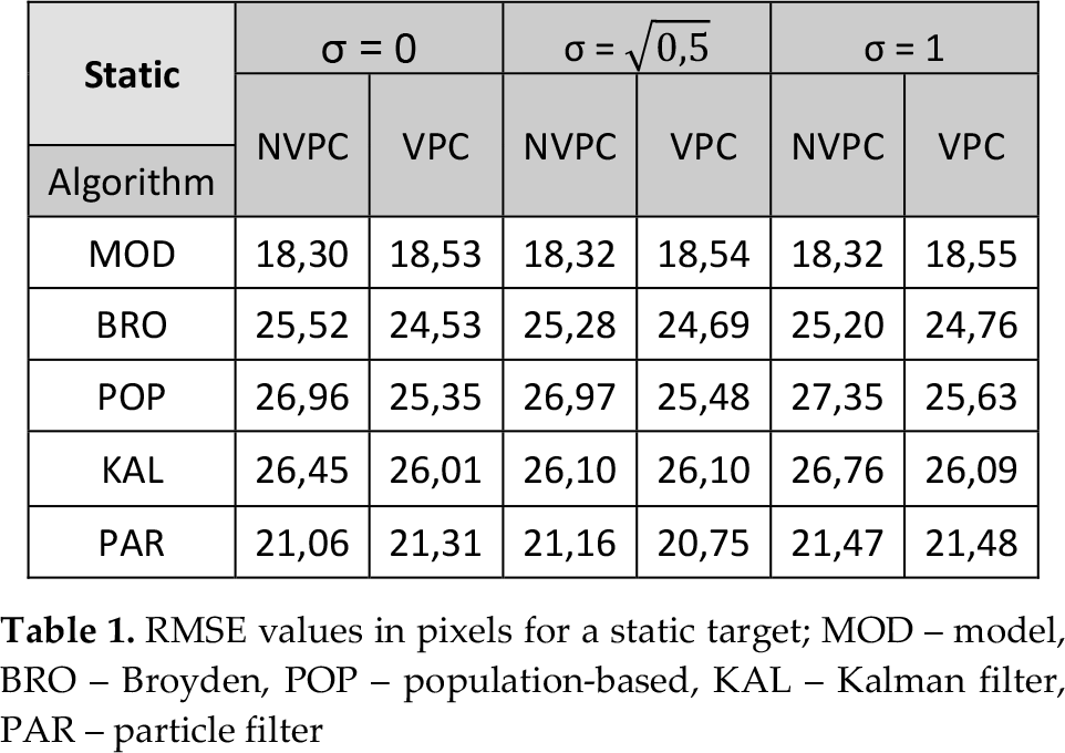
The comparison of the Broyden, population-based and Kalman filter algorithms for static targets showed that the Broyden approach is the most sensible. The differences presented in the table have small absolute values, but it should be kept in mind that this is a simulation and that our experience from previous research [8] suggests that differences are usually amplified in practical applications. It is interesting, visually, to compare the performance of different algorithms, as depicted in Figure 4. However, it should be kept in mind that the RMSE values capture error for all four tracked image features whereas the trajectories presented in Figure 4 pertain only to a single feature.

Figure 4.

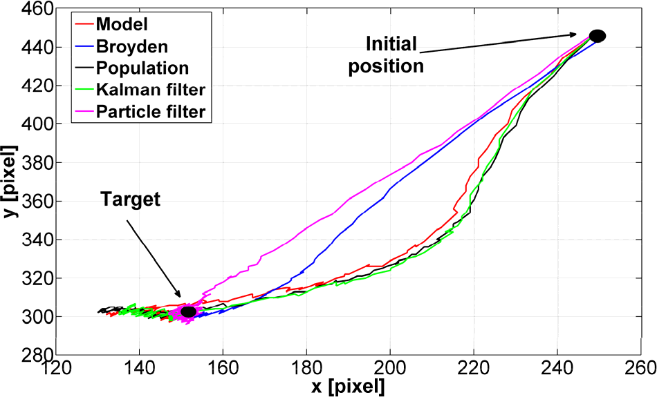
Comparison of 2D trajectory of one feature for static target case with σ² = 0.5 and VPC

Figure 4 provides several additional interesting observations. The particle filter and model-based methods take a more direct approach to the target with little or no overshoot, whereas the other algorithms have a more pronounced overshoot and an indirect approach. When looking at the Broyden, population-based and Kalman filter algorithms, one can see somewhat rugged trajectories. The reason for this is the fact that pixel rounding was used (in conjunction with different sampling times for the controller and camera).

If a sub-pixel accuracy algorithm is employed, a smoother trajectory is obtained – as depicted in Figure 5 – although overshoot is still present. The positive effect of the sub-pixel accuracy algorithm in the case of fine movements toward a static target can also be seen in the obtained RMSE values, which are in every case lower. The improvement varies depending upon the method used, but is generally within the RMSE range of one to two pixels. This is depicted in the bar chart in Figure 6.

Figure 5.

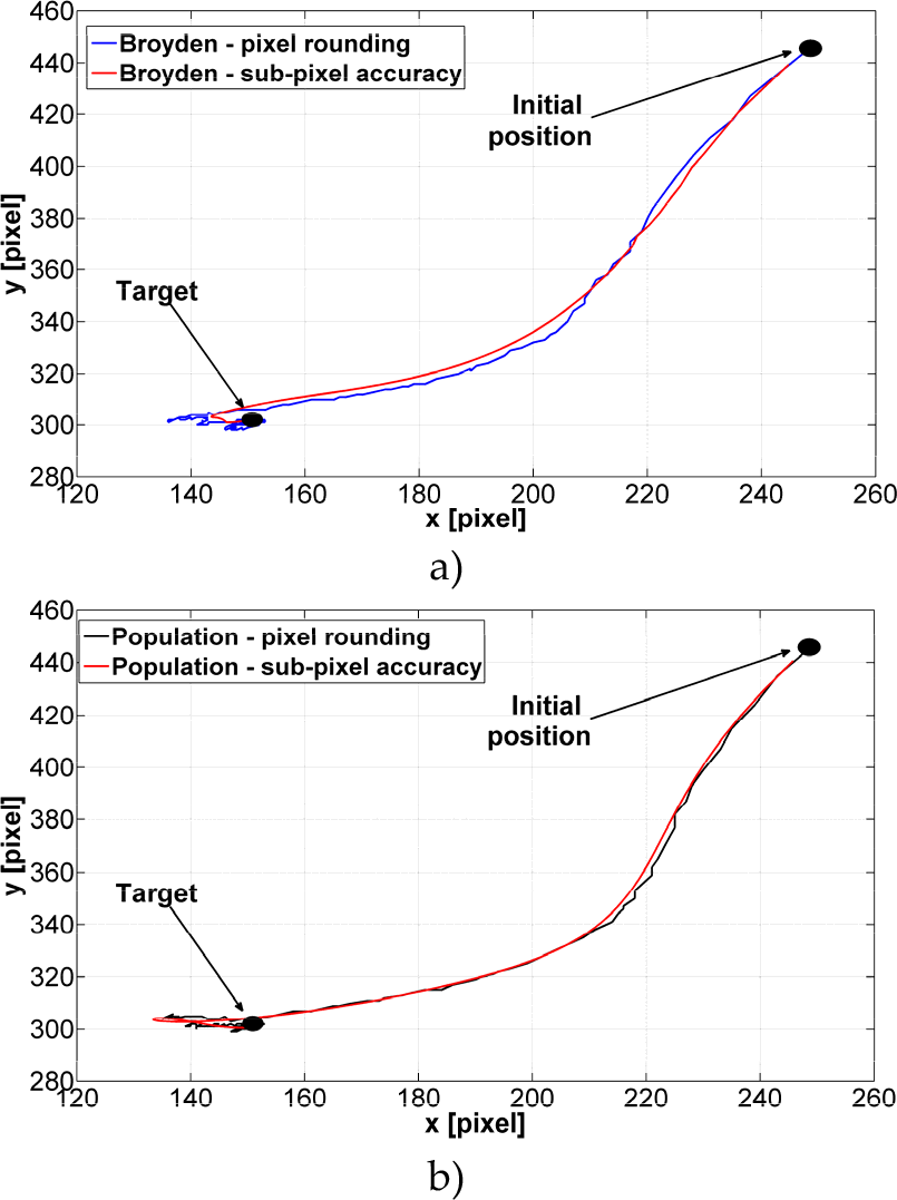
Comparison of the 2D trajectories of the a) Broyden and b) population-based algorithms for one feature with and without a sub-pixel accuracy algorithm for σ² = 0 and VPC.

Figure 6.

Comparison of RMSE values for all methods with and without a sub-pixel accuracy algorithm for σ² = 0 and VPC

4.1.2. Dynamic target-tracking

Rectangular target-tracking was selected as an illustrative example (containing both straight diagonal lines and abrupt changes in direction) of trends in the RMSE values due to article-space constraints. The obtained results are depicted in Table 2. Similar trends in the RMSE values were observed for all other dynamic target trajectories. Here, again, the unfavourable effect of velocity prediction and correction on the model-based method can be observed for all target speeds. Similar trends are present in the RMSE values as in the case of static targets, but with some significant differences. First, the particle filter is again best in terms of accuracy compared with other estimation methods, but again it takes significantly longer to execute. It should, however, be noted that the Broyden method outperforms all other estimation algorithms in the case of a slow-moving target, and with no added noise. As soon as noise is added, the error increases between 15% and 24%, depending upon the measurement conditions. Other methods also exhibit a deterioration in accuracy with the introduction of noise, but it is not so significant, thus highlighting the Broyden algorithm's sensitivity to noise. Please note that the population-based method has the smallest increase in this particular case (a trend which can be observed in all other cases) of about 0.01%.

Table 2.

RMSE values in pixels for dynamic tracking (rectangular-shaped target trajectory)

Rectangle		σ = 0		σ = $\sqrt{0,5}$		σ = 1
Rectangle		NVPC	VPC	NVPC	VPC	NVPC	VPC
S	M	NVPC	VPC	NVPC	VPC	NVPC	VPC
10 pixels/s	MOD	1,72	1,75	1,83	1,8710	1,96	2,00
	BRO	2,83	2,75	3,28	3,2572	3,47	3,40
	POP	3,75	3,10	3,80	3,1008	3,86	3,14
	KAL	3,13	3,00	3,09	3,0614	3,26	3,13
	PAR	3,06	3,09	3,29	3,1786	3,21	3,10
20 pixels/s	MOD	3,00	3,03	3,09	3,1229	3,17	3,21
	BRO	5,28	5,24	5,64	5,5741	5,74	5,79
	POP	6,48	5,62	6,45	5,6895	6,62	5,74
	KAL	5,69	5,53	5,69	5,6196	5,73	5,62
	PAR	4,45	4,48	4,75	4,6761	4,71	4,77
30 pixels/s	MOD	4,19	4,22	4,26	4,2970	4,31	4,34
	BRO	7,43	7,48	7,84	7,8158	7,99	7,96
	POP	8,81	7,99	8,96	8,0327	8,91	8,15
	KAL	8,04	7,86	7,95	7,9931	8,19	8,00
	PAR	6,01	5,87	6,05	5,8695	6,04	5,96

It is also interesting to note that for faster-moving targets the Broyden algorithm in no longer best, even if no noise is present, though it outperforms the population-based and Kalman filter methods. However, the relative increase in the RMSE value is higher than with the other two methods. A population of a different size for population-based method might produce better results. Finding the optimal population size as well as the ideal weighing function is beyond the scope of this paper but is an interesting topic for future research. Additionally, the covariance matrices for the Kalman filter were not adapted to every noise level but were kept constant, which potentially reduced the algorithm's accuracy. The implementation of some type of adaptive mechanism would thus be beneficial. All of this suggests that the Broyden method cannot be recommended when a faster-moving dynamical target is to be tracked, whereas the Kalman filter and population-based methods seem to have similar performance parameter values – the Kalman filter being computationally more efficient. For the purposes of completeness and comparison, a cross-section of the RMSE values of all the methods over all the dynamic target trajectories for a speed of 20 pixels/s is given in Table 3 in the case of VPC and $σ^{2} = 0.5$ .

Table 3.

RMSE values for all methods for all 20 pixels/s dynamic target trajectories in the case of VPC and σ² = 0.5 (L-diagonal line, R – rectangular, C – circle)

		Method
Trajectory		MOD	BRO	POP	KAL	PAR
	L	3,80	5,83	6,14	6,089	4,59
	R	3,12	5,57	5,69	5,62	4,67
	C	2,33	3,83	3,89	3,79	3,42

The visualization of the tracking results for a rectangular target with a 20 pixels/s speed is presented in Figure 7a. Similar trajectory trends to those in the static case can be observed. The particle filter is closest to the model trajectory, although at several places it deviates from it, whereas the Broyden, Kalman and population-based methods have similar trajectories. In particular cases, all the trajectories are rather jittery (even the model-based one) which can be attributed to several reasons: the presence of noise, pixel rounding, different sampling rates of the camera and controller, and small (fine) movements. Thus, our analysis could be considered the worst case scenario. As in the static case, the introduction of sub-pixel accuracy would reduce or even eliminate this effect. To offer a better picture of the algorithms' performances for different trajectories, Figure 7b presents the tracking results for a target's circular trajectory. Similar trends as in the case of the rectangular trajectory can be observed. In the dynamic case, it should be kept in mind that Figure 7 does not explicitly capture time dependency, which makes the direct comparison with the RMSE values somewhat difficult.

Figure 7.

Comparison of the 2D trajectories of one feature for dynamic target-tracking for the case with a speed of 20 pixels/s with σ² = 0.5 and VPC for: a) rectangular target trajectory, and b) circular target trajectory.

4.2. JRK performance

In the context of jittery movements, it is interesting to examine the values and trends in the jerk signal and – possibly – to identify the algorithms which, despite having low RMSE values, might not be suitable for practical applications because of severe mechanical strain on robot joints/actuators. In order to make the analysis and comparison more practical, only the jerk values for the cases presented in subsection 4.1 will be presented here, although similar trends were observed for all the other measurement conditions.

4.2.1. Static target-tracking

The data for static targets are presented in Table 4, the obtained values being within the ranges reported in the literature on robot control applications [40].

Table 4.

Jerk values in rad/s³ for static target.

Static	σ = 0		σ = √0,5		σ = 1
Static	NVPC	VPC	NVPC	VPC	NVPC	VPC
Method	NVPC	VPC	NVPC	VPC	NVPC	VPC
Model	683,6	696,5	658,2	672,7	676,9	702,9
Broyden	586,6	617,1	584,6	470,2	487,4	504,9
Population	447,3	573,9	418,4	443,5	500,9	550,5
Kalman	503,0	506,2	446,1	484,1	503,8	445,9
Particle	1233	1442	1257	1253	12856	1271

Examination of the table reveals that for static cases the particle filter has by far the largest jerk values, although it is the best estimation algorithm. This suggests that the application of the particle filter for static targets might not be the best possible solution if both the RMSE and jerk values are considered. In our opinion, this can be attributed to the nature of the particle filter, which always (even in the vicinity of the actual target) casts a number of particles around the last estimate (amplified if roughening is applied); taking into account the fine nature of the motion under consideration, small oscillations around the target location can be expected (this is also illustrated in Figure 4). The model-based algorithm has the second-highest jerk values, which can be attributed to the fact that it quickly converges on the target location. In general, the population-based algorithm has the lowest jerk values, which was also noted for different robot configurations during experiments in [8]. It is interesting to observe how the robot joint angles change over time for each algorithm. For the third robot joint, this is depicted in Figure 8.

Figure 8.

Comparison of robot third joint angles for the static case with σ² = 0.5 and VPC

In the figure, it can be seen that the two most accurate algorithms (model-based and particle filter) seem to employ slightly different tracking strategies from those in the remaining three methods that differ slightly in their joint angles. This difference is mainly in the form of local minima, which can be traced back to overshoot in the 2D trajectory in Figure 4. Additionally, the existence of slight jitter in the model-based and particle filter signals confirms the data presented in Table 4. However, when comparing Figure 8 and the Table 4 data, one should exercise a certain level of caution since the data in Table 4 are averaged across all robot joints, whereas Figure 8 pertains to only one robot joint (i.e., the other joints might have smaller or larger jerk values).

For the jerk parameter, we were also interested in whether sub-pixel accuracy would reduce (or increase) its values. As depicted in Figure 9, the inclusion of sub-pixel accuracy dramatically reduced the jerk values (please note that because of large amplitude differences, the y axis is presented in natural logarithmic form). Negative values indicate that in some cases it was lower than one. This again demonstrates the positive effects that sub-pixel accuracy can have on final robot performance and justifies its inclusion in the loop. These effects are even more dramatic if the robot joint angles are examined. In Figure 10, the joint angles for the robot's third joint are presented.

Figure 9.

Comparison of jerk values for all methods with and without the sub-pixel accuracy algorithm for σ² = 0 and VPC

Figure 10.

Comparison of robot third joint angles for the a) model- based and b) Kalman filter algorithms with and without the sub-pixel accuracy algorithm for σ² = 0 and VPC.

4.2.2. Dynamic target-tracking

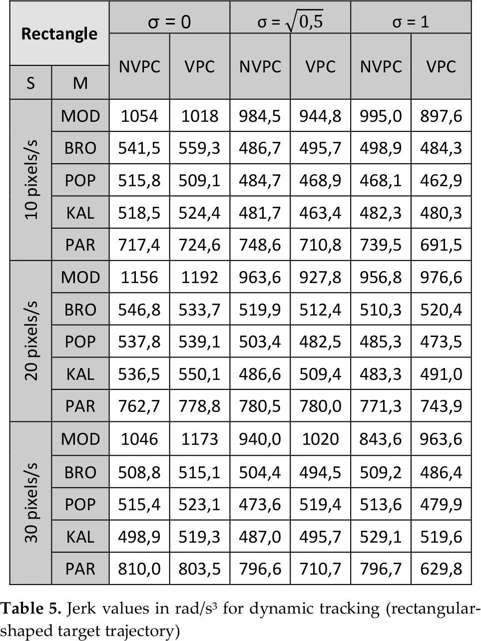
If dynamic target-tracking is examined and the rectangle trajectory is selected as a representative example, then the data shown in Table 5 are obtained. It is interesting to note that, now, the model-based algorithm has the largest jerk values, which again could be attributed to its tracking speed. The particle filter has significantly smaller values than in the static case (supporting our explanation with respect to static targets), but they are still larger than in the case of the remaining three estimation algorithms. The population-based method again generally has the smallest jerk values, except with regard to high-speed targets (in which case, the Kalman filter and Broyden method would seem to be a better choice). This in turn suggests that the population-based method (at least in the current configuration) might be better suited for slower-moving targets. Looking at the third robot joint angle values in Figure 11, we can draw similar conclusions to those in the static case.

Figure 11.

Comparison of robot third joint angles dynamic target-tracking for a rectangular target trajectory and a speed of 20 pixels/s with σ² = 0.5 and VPC

Table 5.

Jerk values in rad/s³ for dynamic tracking (rectangular-shaped target trajectory)

Rectangle		σ = 0		σ = √0,5		σ = 1
Rectangle		NVPC	VPC	NVPC	VPC	NVPC	VPC
S	M	NVPC	VPC	NVPC	VPC	NVPC	VPC
10 pixels/s	MOD	1054	1018	984,5	944,8	995,0	897,6
	BRO	541,5	559,3	486,7	495,7	498,9	484,3
	POP	515,8	509,1	484,7	468,9	468,1	462,9
	KAL	518,5	524,4	481,7	463,4	482,3	480,3
	PAR	717,4	724,6	748,6	710,8	739,5	691,5
20 pixels/s	MOD	1156	1192	963,6	927,8	956,8	976,6
	BRO	546,8	533,7	519,9	512,4	510,3	520,4
	POP	537,8	539,1	503,4	482,5	485,3	473,5
	KAL	536,5	550,1	486,6	509,4	483,3	491,0
	PAR	762,7	778,8	780,5	780,0	771,3	743,9
30 pixels/s	MOD	1046	1173	940,0	1020	843,6	963,6
	BRO	508,8	515,1	504,4	494,5	509,2	486,4
	POP	515,4	523,1	473,6	519,4	513,6	479,9
	KAL	498,9	519,3	487,0	495,7	529,1	519,6
	PAR	810,0	803,5	796,6	710,7	796,7	629,8

The model-based and particle filter algorithms employ different dynamic target-tracking strategies from those employed by the remaining three estimation algorithms, which all have similar angle profiles. It is also interesting to note that although the model-based and particle filter approaches have dramatically different joint angles in the third robot joint, their feature trajectory in the image plane (as depicted in Figure 7) is not significantly different. Small oscillations in the trajectories of the model-based approach (especially around 12 s to 18 s) and the particle filter algorithms in a sense support the data in Table 5. As in the case of the RMSE values, a cross-section of the jerk values for all the estimation algorithms and all the dynamic target trajectories with a speed of 20 pixels/s with VPC and $σ^{2} = 0.5$ are given for completeness and comparison purposes in Table 6.

Table 6.

JRK values for all the methods, all with a speed of 20 pixels/s and dynamic target trajectories with VPC and σ² = 0.5

		Method
Trajectory		MOD	BRO	POP	KAL	PAR
	L	683,62	504,49	497,86	473,21	446,15
	R	927,76	512,41	482,48	509,43	780,02
	C	542,52	511,35	497,08	499,13	583,43

The fusion of all the obtained results suggests that it might prove beneficial to have a switching logic which would, depending upon the target trajectory shape (and taking into account the convergence rate of every algorithm), switch between different estimation algorithms. Such a switching logic would act as a kind of supervisor which would decide which method is appropriate in a particular case. A similar logic (but for a different application) was used in [29].

To demonstrate the validity of this assumption, we created a trajectory consisting of four simpler ones with known start- and end-time instances: a diagonal line, a static point and two one-directional lines (in the x and y directions). Three cases were tested: Broyden only, particle filter only, and a combination of Broyden and particle filter, where the Broyden method was used in part of the static target and the particle filter in the other three characteristic trajectories.

The obtained results in terms of the RMSE and jerk values are presented in Table 7, from which it can be seen that switching has a potentially compromising effect. It should also be noted that the switching algorithm also reduced the computational cost in comparison with the particle filter alone.

Table 7.

Comparison of the Broyden method, the particle filter and the Broyden-particle filter combination (COMBO) results

		BRO	PAR	COMBO
Diagonal	RMSE	8,28	5,62	5,69
Diagonal	JRK	582,42	408,01	433,24
Static	RMSE	9,45	1,32	1,21
Static	JRK	338,83	1576,60	332,32
One directional lines	RMSE	7,04	4,49	4,42
One directional lines	JRK	570,22	551,96	545,23

4.3. 2D two-sample Kolmogorov-Smirnov test

Presenting the results of all the tests is not possible because of space-constraints, but some interesting conclusions can be drawn and some illustrative examples presented. It is important to note that although some methods (within and between method comparisons) exhibited different accuracy levels in Table 1 and Table 2, this did not necessarily reflect in the statistical tests performed. This is indicative of the RMSE vs. trajectory-shape relation explained in section 3.3.

If, within the algorithm, comparison is made, the following conclusion can be drawn:

–

Model-based approach: in the static case, there is a statistically significant difference for cases when there is no noise, but with the introduction of noise this effect disappears. The same effect is present in the following dynamical cases: line slow (10 pixel/s) and line fast (30 pixel/s). In all other cases, no statistically significant difference was detected.

–

Broyden method: the only statistically significant difference was detected in the static target case when we compared trajectories generated in the case of no noise and without VPC with other trajectories.

–

Population-based method: no statistically significant difference was detected.

–

Kalman filter: in the static case, a difference was observed when we compared cases with no noise (with and without VPC) with cases with $σ^{2} = 1$ , and when we compared cases with no noise and VPC with cases with $σ^{2} = 0.5$ and no VPC. No difference was detected in any other case.

–

Particle filter: in the static case, a difference was observed in comparison with VPC and no noise with all other cases, whereas in the dynamic tracking scenario a difference was observed in the case of fast-moving targets (line and rectangular trajectories) with the following noise-VPC combinations: the line-no noise-VPC case with line- $σ^{2} = 0.5$ -VPC and the line- $σ^{2} = 1$ -VPC cases; rectangular-no noise-VPC with rectangular-no noise-no VPC, rectangular- $σ^{2} = 0.5$ -VPC and rectangular- $σ^{2} = 1$ -VPC cases.

To offer a clearer picture of the algorithms' discriminatory power we present two cases in Figure 12 for the particle filter method in similar dynamic target-tracking scenarios.

Figure 12.

Illustration of statistically significant test results for the particle filter tracking of a target moving at 30 pixels/s. The blue trajectory, according to two sample 2D Kolmogorov-Smirnov tests, is statistically different at the 0.05 level with respect to the red trajectory, but red is not different from the green trajectory.

When we compared the algorithms using only cases with the same noise and VPC status parameters, we made the following observations:

–

No noise: in general, the model-based approach (VPC and NVPC) was significantly different from all other methods in the static case and for slow and fast line trajectories. Differences were also detected in normal (20 pixel/s) and fast rectangular and circular target trajectories. The Broyden method generally demonstrated a difference only with the particle filter algorithm in the static case and in the fast speed line and rectangular cases. The same was true of the population-based method with a rectangular trajectory and normal speed. The Kalman filter exhibited a statistically significant difference in comparison with the particle filter method in the static case, for slow and fast line trajectories, and for normal and fast rectangular trajectories.

–

Noise with $σ^{2} = 0.5$ : in general, the model-based approach demonstrated a difference from all the other cases in relation to a static target and a line target trajectory. A difference was also observed for a fast rectangular trajectory in comparison with the particle filter, as well as for normal and fast circular target trajectories with respect to the particle filter. The Broyden method was different from the particle filter in the static case, slow and normal target speed for straight line case only with VPC and in fast line target trajectory. For the rectangular case, a difference was observed only for a fast target speed, and no difference in the circular trajectories was detected. The Kalman filter demonstrated a statistical difference in respect to the particle filter in the static case with a fast line trajectory and a fast rectangular trajectory.

–

Noise with $σ^{2} = 1$ : in general, the model-based approach demonstrated a difference from all the other cases in relation to the static target. For line trajectories, a difference was present only for fast targets. No differences were observed for the rectangular and circular trajectories. The Broyden algorithm a demonstrated difference from the population-based and Kalman filter algorithms in the case of VPC, and from the particle filter in both the VPC and NVPC static cases. A difference from the particle filter output was also detected in fast line tracking. The population-based method exhibited a statistically significant difference from the particle filter in the static case with fast line and fast rectangular trajectories. The same held for the Kalman filter.

Finally, the statistical differences of the generated trajectories in the static target case (with no noise) were examined for outputs with pixel rounding and sub-pixel accuracy. Comparison was made with corresponding measurements only. In every case, a very significant statistical difference was observed.

5. Conclusions

This paper compared several methods for the estimation of an image Jacobian used for visual servoing in an eye-in-hand configuration in the simulation study of a number of application scenarios. This large number of experimental scenarios coupled with four estimation algorithms and a model-based approach provided a large amount of data. The data were used for drawing conclusions based on three performance parameters: the root mean square error, jerk and the statistical difference of observed 2D trajectories. Although not quantitatively analysed, the influence of computation time was observed. The obtained results suggest that no single method can be applied in all scenarios and with all performance parameters in mind. Thus, a between-algorithm switching technique was proposed and initially tested to prove the validity of the assumptions made.

In the static case, the model-based approach was best in terms of accuracy, followed by the particle filter; however, the particle filter had higher jerk values than the model-based approach. The computational time of the particle filter was up to six times that of the Broyden method. Particle filter jerkiness was greatly reduced in the dynamic scenarios, which we attributed to the nature of the filter. Accuracy levels generally showed the same trends in dynamic cases as in static cases, but it was evident that the Broyden method is by far the most sensitive to noise while the population-based method is not. This is not surprising, since its operation is based on the number of past estimations, thus significantly reducing the influence of noise. It is interesting to note that the Broyden algorithm performed better in terms of RMSE values in dynamic line target-tracking in the diagonal direction (i.e., when both the x and y coordinates changed) than when one directional motion was considered (i.e., when one coordinate was kept constant and the other one changed).

A slight difference in algorithm performance was observed in dynamic cases, depending upon the target trajectory as well as upon the target speed. Statistically significant testing showed that, for smaller speeds, although there is a difference in the RMSE values, the resulting trajectories were not different, and this was not true for faster speeds. This might be because RMSE implicitly takes time into account, whereas statistical testing does not. Additionally, a few differences were detected for circular target motion. It should also be noted that the inclusion of the VPC algorithm improved the performance of all the estimation algorithms except for the model-based algorithm, and that the population-based approach showed the greatest deterioration in accuracy when VPC was turned off.

Finally, we tested in limited number of cases what effect the sub-pixel accuracy algorithm would have on the performance of the visual servoing algorithms. The obtained results demonstrated a significant impact on all the parameters: the RMSE error was slightly reduced, jerk was significantly reduced, and a statistical difference was observed between the corresponding pixel-rounding and sub-pixel algorithm cases. All of this suggests that the inclusion of this kind of algorithm is desirable in any type of visual servoing.

It should be pointed out that this was a simulation study and that the experiment should be repeated on a real robot (or a number of them), which is one of our future research directions. The selection of optimal parameters for estimation methods is another important area where improvements in performance might be achieved. Additional future research directions include testing under additional dynamic target motion trajectories, the implementation of a switching supervisor, and the development of an adaptive weighing function for the population-based algorithm.

References

Shirai

& Inoue

(1973) Guiding a robot by visual feedback in assembling tasks, Pattern Recogn. 5: 99–108.

Hill

& Park

(1979) Real time control of a robot with a mobile camera, In: Wallace

John J.

, editor. 9^th International Symposium on Industrial Robots. 1979 Mar 13-15, Washington D. C., USA. Washington: SME. pp. 223–246.

Weiss

L. E.

Sanderson

A. C.

& Neuman

C. P.

(1987) Dynamic Sensor-Based Control of Robots with Visual Feedback, IEEE T. Robotic. Autom. 3: 404–417.

Hosoda

& Asada

(1994) Versatile visual servoing without knowledge of true Jacobian, In: IEEE/RSJ/GI International Conference on Intelligent Robots and Systems (IROS). 1994 Sep 12-16, New York, Germany. Munich: IEEE, Vol. 1, pp. 186–193.

Jägersand

& Nelson

(1996) On-line Estimation of Visual-Motor Models using Active Vision, In: ARPA Image Understanding Workshop, 1996 Feb 12-15, Palm Springs, USA. San Francisco: Morgan Kaufmann Publishers. pp. 677–682.

Sutanto

Sharma

& Varma

(1998) The role of exploratory movement in visual servoing without calibration, Robot. Auton. Syst. 23: 153–169.

Kragic

& Christensen

H. I.

(2002) Survey on Visual Servoing for Manipulation [Technical Report]. Stockholm: Royal Institute of Technology.

Bonkovic

Hace

& Jazernik

(2008) Population-Based Uncalibrated Visual Servoing, IEEE/ASME T. Mech. 13: 393–397.

Hao

& Sun

(2012) A Universal State-Space Approach to Uncalibrated Model-Free Visual Servoing, IEEE/ASME T. Mech. 17: 833–846.

10.

Broyden

C. G.

(1965) A class of methods for solving nonlinear simultaneous equations, Math. Comput. 19: 577–593.

11.

Zeng

& Zhou

(1998) Convergence of Broyden-like matrix, Appl. Math. Lett. 11: 35–37.

12.

Piepmeier

J. A.

McMurray

G. V.

& Lipkin

(2004) Uncalibrated Dynamic Visual Servoing, IEEE T. Robotic. Autom. 20: 143–147.

13.

Khan

Jan

Iqbal

& Dai

(2011) Uncalibrated eye-in-hand visual servoing: an LMI approach, Ind. Robot. 39: 130–138.

14.

Sebastian

J. M.

Pari

Angel

& Traslosheros

(2009) Uncalibrated visual servoing using the fundamental matrix, Robot. Auton. Syst. 57: 1–10.

15.

Chaumette

& Hutchinson

(2006) Visual servo control Part I: Basic Approaches, IEEE Robot. Autom. Mag. 13: 82–90.

16.

Chaumette

& Hutchinson

(2007) Visual servo control Part II: Advanced Approaches, IEEE Robot. Autom. Mag. 14: 109–118.

17.

Janabi-Sharifi

Deng

& Wilson

W. J.

(2011) Comparison of Basic Visual Servoing Methods, IEEE/ASME T. Mech. 16: 967–983.

18.

Malis

Chaimette

& Bouder

(1999) 2 1/2 D visual servoing, IEEE T. Robot. and Autom. 15: 234–246.

19.

Piepmeier

J. A.

& Lipkin

(2003), Uncalibrated Eye-in-Hand Visual Servoing, Int. J. Robot. Res. 22: 805–819.

20.

Kosmopoulos

(2011) Robust Jacobian matrix estimation for image-based visual servoing, Robot. CIM-Int. Manuf. 27: 82–87.

21.

Shademan

Farahmand

A.-M.

& Jägersand (2010) Robust Jacobian Estimation for Uncalibrated Visual Servoing, In: IEEE International Conference on Robotics and Automation (ICRA). 2010 May 3-8, Anchorage, USA. IEEE: Anchorage. pp. 2874–2880.

22.

Kim

G.-W.

(2013) Uncalibrated Visual Servoing through the Efficient Estimation of the Image Jacobian for Large Residuals, J. Electr. Eng. Technol. 8: 385–392.

23.

Santamaria-Navarro

& Andrade-Cetto

(2013) Uncalibrated image-based visual servoing, In: IEEE International Conference on Robotics and Automation (ICRA). 2013 May 6-10, Karlsruhe, Germany, IEEE: Karlsruhe. pp. 5247–5252.

24.

Chen

Zhu

Wang

& Wu

(2012) Analysis on an uncalibrated image-based visual servoing for 6 DOF industrial welding robots, In: IEEE International Conference on Mechatronics and Automation (ICMA). 2012 Aug 5-8, Chengdu, China, IEEE: Chengdu. pp. 2013–2018.

25.

Qian

& Su

(2002) Online estimation of image Jacobian matrix by Kalman-Bucy filter for uncalibrated stereo vision feedback, In: IEEE International Conference on Robotics and Automation (ICRA). 2002 May 11-15, Washington D.C., USA, Washington, IEEE: pp. 562–567.

26.

Hafez

A. H. A.

& Jawahar

C. V.

(2006) Target Model Estimation using Particle Filters for Visual Servoing, In: 18^th International Conference on Pattern Recognition (ICPR). 2006 Aug 20-25, Hong Kong, China, IEEE Computer Society: Los Alamitos. Vol. 4, pp. 651–654.

27.

Fiococelli

& Janabi-Sharifi

(2001) Adaptive Filtering for Pose Estimation in Visual Servoing, In: IEEE/RSJ International Conference on Intelligent Robots and Systems (IROS). 2001 Oct 29 – Nov 3, Maui, USA, IEEE: Maui. pp. 19–24.

28.

Lippiello

Siciliano

& Villani

(2007) Adaptive extended Kalman filtering for visual motion estimation of 3D objects, Control Eng. Pract. 15: 123–134.

29.

Hashimoto

Nagahama

& Noritsugu

(2002) A Mode Estimation for Visual Servoing, In: IEEE International Conference on Robotics & Automation (ICRA). 2002 May 11-15, Washington D.C., USA, Washington, IEEE: pp. 1610–1615.

30.

Chaumette

(1998) Potential problems of stability and convergence in image-based and position-based visual servoing, In: Conference of Vision and Control, Lect. Notes Contr. Inf. 237: 66–78.

31.

Miura

(2004) Robot Hand Positioning and Grasping Using Vision [PhD Thesis]. Strasbourg: Strasbourg I University.

32.

Hao

Deuflhard

Sun

& Fujii

(2008) Model-free Uncalibrated Visual Servoing Using Recursive Least Squares, J. Comput. 3: 11–43.

33.

Corke

(1996) A robotics toolbox for MATLAB, IEEE Robot. Autom. Mag. 3: 24–32.

34.

Campoy

Mondragon

I. F.

Olivares-Mendez

M. A.

& Martinez

(2010) Visual servoing for UAVs, Visual servoing. In: Fung

Rong-Fong

Editor. Visual Servoing. Rijeka: InTech. pp. 181–216.

35.

Simon

(2006) Optimal State Estimation: Kalman, H Infinity, and Nonlinear Approaches. New Jersey, USA: Wiley-Interscience. pp. 123–326.

36.

Ristic

Arulampalam

& Gordon

(2004) Beyond the Kalman Filter: Particle Filters for Tracking Applications. Boston, USA: Artech House. pp. 1–62.

37.

Bolic

Djuric

& Hong

(2004) Resampling Algorithms for Particle Filters: A Computational Complexity Perspective, EURASIP J. Adv. Sig. Pr. 2004: 2267–2277.

38.

Lopes

R. H. C.

Reid

& Hobson

P. R.

(2007) The two-dimensional Kolmogorov-Smirnov test, In: XI International Workshop on Advanced Computing and Analysis Techniques in Physics Research, 2007 Apr 23-27, Amsterdam, Holland, Proceedings of Science. Available from: http://pos.sissa.it/archive/conferences/050/045/ACAT_045.pdf. Accessed on 01 Feb 2014.

39.

Babu

G. J.

& Feigelson

E. D.

(2005) Astrostatistics: Goodness-of-Fit and All That! In: XV Astronomical Data Analysis Software and Systems, 2005 Oct 2-5, San Lorenzo de El Escorial, Spain. San Francisco: Astronomical Society of the Pacific. Vol. 351, pp. 127.

40.

Rubio

Valero

Sunyer

& Cuadrado

(2012), Optimal time trajectories for industrial robots with torque, power, jerk and energy consumed constraints, Ind. Robot. 39: 92–100.

Comparison of Uncalibrated Model-Free Visual Servoing Methods for Small-Amplitude Movements: A Simulation Study

Abstract

Keywords

1. Introduction

2. Image-based visual servoing – A brief literature review

3. Materials and methods

3.1. Experimental setup

3.2. Image Jacobian estimation algorithms

3.2.1. Analytical estimation of the Jacobian matrix

3.2.2. The Broyden method

3.2.3. The population-based method

3.2.4. The Kalman filter

3.2.5. The particle filter

3.3. Evaluation methods

4. Simulation results and discussion

4.1. RMSE performance

4.1.1. Static target-tracking

4.1.2. Dynamic target-tracking

4.2. JRK performance

4.2.1. Static target-tracking

4.2.2. Dynamic target-tracking

4.3. 2D two-sample Kolmogorov-Smirnov test

5. Conclusions

References