Closed-form camera pose and plane parameters estimation for moments-based visual servoing of planar objects

Abstract

Image moments are global descriptors of an image and can be used to achieve control-decoupling properties in visual servoing. However, only a few methods completely decouple the control. This study introduces a novel camera pose estimation method, which is a closed-form solution, based on the image moments of planar objects. Traditional position-based visual servoing estimates the pose of a camera relative to an object, but the pose estimation method directly estimates the pose of an initial camera relative to a desired camera. Because the estimation method is based on plane parameters, a plane parameters estimation method based on the 2D rotation, 2D translation, and scale invariant moments is also proposed. A completely decoupled position-based visual servoing control scheme from the two estimation methods above was adopted. The new scheme exhibited asymptotic stability when the object plane was in the camera field of view. Simulation results demonstrated the effectiveness of the two estimation methods and the advantages of the visual servo control scheme compared with the classical method.

Introduction

Visual servoing control refers to the use of computer vision data to control the motion of a robot. ¹ In visual servoing, two closely linked problem themes are subjects of active research ² : the design of visual features pertinent to the robotic task to be realized and a control scheme with the chosen visual features such that the desired characteristics are obtained during visual servoing. The latter adopts the control scheme of ensuring an exponential decoupled decrease in error. The former employs the observed parameters of the visual feature in the image of geometric primitives (points, straight lines, ellipses, and cylinders) in image-based visual servoing (IBVS). ^{3 –5} In position-based visual servoing (PBVS), ^{6 –8} the geometric primitives reconstruct the camera pose, which then serves as input for visual servoing. The above approaches subject the image stream to an ensemble of measurement processes, including image processing, image matching, and visual tracking steps, from which the visual features are determined. ⁹ With large measurement errors, PBVS can be affected by instability in pose estimation and IBVS designed from the image points is subject to local minima, singularity, and limited convergence domain. ¹⁰ This is due to the image mismatch, strong nonlinearities, and coupling in the interaction matrix of image points. As a solution to these issues, image moments were introduced for visual servoing. ^{11 –14}

Image moments have a broad spectrum of applications in image analysis, such as invariant pattern recognition, ^15,16 pose estimation, ^17,18 and reconstruction. ¹⁹ A set of moments computed from a digital image represents the global characteristics of the image shape and provides much information regarding the different geometrical features of the image. ²⁰ Because the descriptors used are global and nongeometrical, they avoid image processing such as feature extraction, matching, and tracking. ¹⁸ Moments are also useful in achieving control-decoupling properties and choosing a minimal number of features to control the whole degrees of freedom of a camera. Therefore, visual servoing using image moments obtains a large convergence domain and adequate robot trajectories, because of the reduced nonlinearities and coupling in interaction matrix of the adequate combinations of moments.

The analytical form of the interaction matrix related to any moment generated from segmented images was determined, and the result was applied to classical geometric primitives. ¹¹ However, this method requires an object plane configured such that the object and camera planes are parallel to the desired position. Another drawback is the strong coupling of the interaction matrix. Tahri and Chaumette ¹² designed a decoupled control scheme to weaken the coupling of the visual features and functions when the object is parallel to the image plane. A generalization of the aforementioned property, that is, when the desired object position is unparallel to the image plane, has achieved excellent experimental results, but it should determine what virtual rotation to apply to the camera and that the x- and y-axes angular velocities of the camera are still coupled. To solve the problem of selecting the image moments to control the rotational motions around the x- and y-axes simultaneously with the translational motions along the same axis, new visual features computed from a low-order shifted moment invariant are proposed. ¹³ On the basis of the shifted moments, the selection of a unique feature vector independent of the object shape is proposed and exploited in IBVS. Although this method significantly enlarges the convergence domain of the closed-loop system, the interaction matrix is also coupled. The above methods are all IBVS schemes. Presently, few studies on PBVS control schemes based on image moments exist, but the hybrid visual servoing is very popular. A novel moment-based 2 1/2D visual servoing method for grasping textureless planar parts is proposed by He et al. ¹⁴ Instead of applying high-order image moments, it uses rotation features, providing a decoupled interaction matrix that has a full rank and has no local minimum in the control scheme. However, the estimation method of the relative rotation of the textureless parts in real time is based on the cross-correlation analysis and is not a closed-form solution.

To handle the above issues more effectively, this study proposes a closed-form solution of camera pose estimation based on the image moments of planar objects. This method directly estimates the relative pose of the initial camera and the desired camera and not the pose of the camera relative to the object plane. Because the estimation method follows plane parameters, a plane parameters estimation method based on invariant moments is also proposed. Finally, we adopted the PBVS control scheme, which has a completely decoupled interaction matrix.

The rest of the article is organized as follows. The second section discusses preliminary knowledge; the third section introduces camera pose estimation based on image moments; the fourth section is devoted to plane parameters estimation based on the invariant moments; the fifth section discusses the PBVS control scheme and stability analysis; the sixth section presents the simulation results obtained from the co-simulation of MATLAB and CoppeliaSim; and finally, the seventh section outlines the conclusions and future work.

Preliminaries

This section introduces the preliminary knowledge used in this study. The pinhole camera model and imaging geometry are introduced, which play important roles in deriving formulas. Then, the relationships between the image moments of two cameras are described, laying the foundation for two camera pose estimation.

The pinhole camera model and imaging geometry

From the pinhole camera mode, ²¹ for a 3D coordinate $P={\left[X,Y,Z\right]}^{\text{T}}$ in the camera frame, which projects images as 2D homogeneous normalized coordinates $p={\left[x,y\mathrm{,1}\right]}^{\text{T}}$ , we have $p=P/Z$ . The image plane measurement (in pixels) of points is given by $\overline{p}={\left[p_u,p_v\mathrm{,1}\right]}^{\text{T}}$ . The relationship between $p$ and $\overline{p}$ is expressed as $p=K^{-1}\overline{p}$ , where $K$ is a nonsingular matrix containing the intrinsic parameters of the camera. ²² To simplify the notation, we will assume that any quantity is expressed in the normalized space. This is equivalent to assuming a calibrated camera, that is, full knowledge of the calibration matrix $K$ .

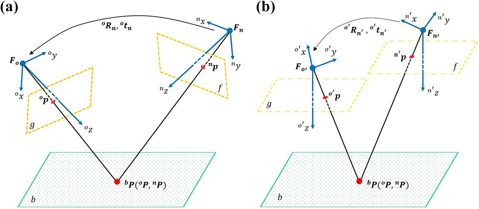
The homogeneous normalized coordinates of the two camera image points in Figure 1(a) are ${ }^{n}p={\left[{ }^{n}x{,}^{n}y\mathrm{,1}\right]}^{\text{T}},{}^{o}p={\left[{ }^{o}x{,}^{o}y\mathrm{,1}\right]}^{\text{T}}$ , satisfying a certain relationship. Assuming that point ${ }^{b}P$ on planar b is represented as ${ }^{n}P$ and ${ }^{o}P$ in the camera frames $F_n$ and $F_o$ , respectively, then ${ }^{n}p$ and ${ }^{o}p$ satisfy

${ }^n{Z}^{n}p{=}^{n}P$

1

${ }^o{Z}^{o}p{=}^{o}P{=}^o{R}_n{ }^{n}P{+}^o{t}_n$

2

where ${ }^{n}Z$ and ${ }^{o}Z$ are the depth of the observed point ${ }^{b}P$ relative to the camera frames $F_o$ and $F_n$ , respectively, and ${ }^o{R}_n$ and ${ }^o{t}_n$ are the rotation matrix and translation vector of the camera frame $F_n$ relative to the camera frame $F_o$ , respectively. Substituting for ${ }^{n}P$ using equation (1), equation (2) can be written as

${ }^{o}p={\frac{{ }^{n}Z}{{ }^{o}Z}}^o{R}_n^{n}p+\frac{{ }^o{t}_n}{{ }^{o}Z}$

3

Figure 1.

Basic geometry for two images: (a) the imaging plane is not parallel to the object plane and (b) the imaging plane is parallel to the object plane.

The following will only consider a planar or has a planar limb surface. Here, the depth Z of any object plane can be expressed as a continuous function of its image coordinates (see the study of Espiau and Chaumette ³ for more details) and as follows

$\frac{1}{Z}=Ax+By+C$

4

where A, B, and C are the object plane parameters, and we define $N={\left[ABC\right]}^{\text{T}}$ . The parameters of a plane containing typical primitives has been studied by Espiau and Chaumette ³ and Chaumette et al. ²³ To find the parameters of a plane containing any pattern, the general method for estimating plane parameters based on the invariant moments will be introduced in the fourth section.

Image moments

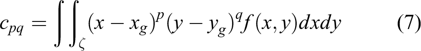
Moments are generic (and intuitive) descriptors computed from several kinds of objects defined either from closed contours or from a set of points. The ${\left(p+q\right)}^{\text{th}}$ order 2D geometric moments are denoted by $m_{pq}$ and can be expressed as

$m_{pq}={\displaystyle {\iint }_{\zeta }}{x}^p{y}^{q}f\left(x,y\right)dxdy,\forall p,q\in \mathbb{N}$

5

where $\zeta$ is the region of the normalized space in which the image intensity function $f\left(x,y\right)$ is defined. The intensity centroid $\left(x_g,y_g\right)$ is given by

$x_g=\frac{m_{10}}{m_{00}},y_g=\frac{m_{01}}{m_{00}}$

6

The moments computed with respect to the intensity centroid are called centered moments and are defined as

$c_{pq}={\displaystyle {\iint }_{\zeta }}{\left(x-x_g\right)}^p{\left(y-y_g\right)}^{q}f\left(x,y\right)dxdy$

7

The following considers objects defined by a binary region. Therefore, we assume that $f\left(x_i,y_j\right)=1$ in all the region that defines the object.

In the studies of Espiau and Chaumette ³ and Chaumette, ¹¹ the interaction matrix $L_{c_{pq}}$ related to any centered moment defined from equation (7) has been determined. So we can get

${\dot{c}}_{pq}=L_{c_{pq}}{v}_c$

8

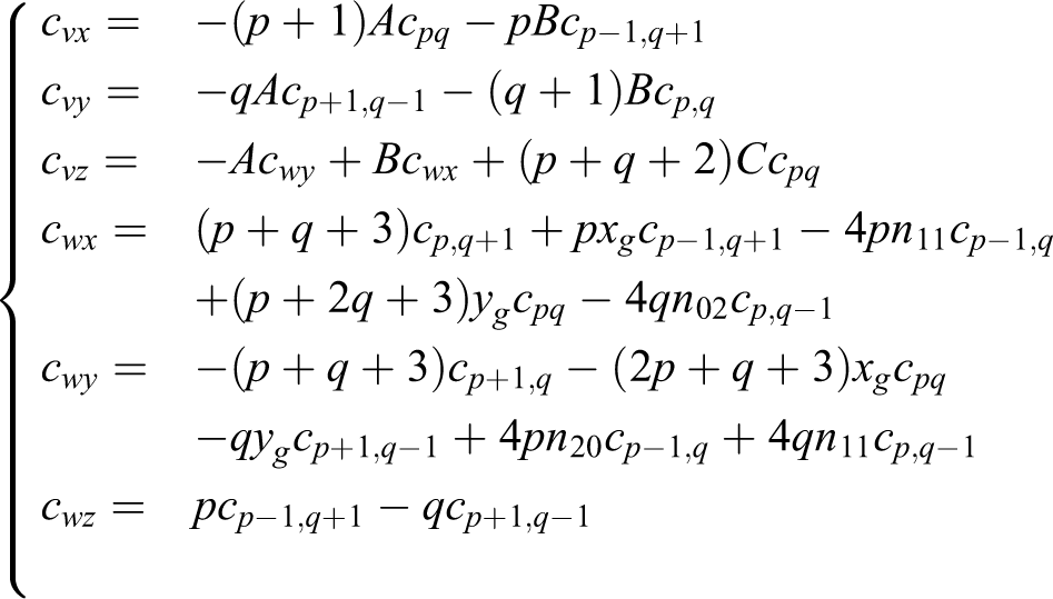
where the relative kinematic screw $v_c={\left[{\nu }_c{\omega }_c\right]}^{\text{T}}$ between the camera and the object, where ${\nu }_c$ and ${\omega }_c$ represent the translational and rotational velocity components, respectively. And the interaction matrix $L_{c_{pq}}$ can be calculated as

$L_{c_{pq}}=\left[c_{vx}{c}_{vy}{c}_{vz}{c}_{wx}{c}_{wy}{c}_{wz}\right]$

where

$\{\begin{array}{ll}{c}_{vx}=\hfill & -\left(p+1\right)A{c}_{pq}-pB{c}_{p-1,q+1}\hfill \\ c_{vy}=\hfill & -qA{c}_{p+1,q-1}-\left(q+1\right)B{c}_{p,q}\hfill \\ c_{vz}=\hfill & -A{c}_{wy}+B{c}_{wx}+\left(p+q+2\right)C{c}_{pq}\hfill \\ c_{wx}=\hfill & \left(p+q+3\right)c_{p,q+1}+p{x}_g{c}_{p-1,q+1}-4p{n}_{11}{c}_{p-1,q}\hfill \\ \hfill & +\left(p+2q+3\right)y_g{c}_{pq}-4q{n}_{02}{c}_{p,q-1}\hfill \\ c_{wy}=\hfill & -\left(p+q+3\right)c_{p+1,q}-\left(2p+q+3\right)x_g{c}_{pq}\hfill \\ \hfill & -q{y}_g{c}_{p+1,q-1}+4p{n}_{20}{c}_{p-1,q}+4q{n}_{11}{c}_{p,q-1}\hfill \\ c_{wz}=\hfill & p{c}_{p-1,q+1}-q{c}_{p+1,q-1}\hfill \\ \hfill & \hfill \end{array}$

where $n_{pq}$ is defined as $n_{pq}=c_{pq}/c_{00}$ .

Relationship between the image moments of two cameras

If two cameras are not parallel to the object plane (see Figure 1(a)), then ${ }^{n}Z$ and ${ }^{o}Z$ in equation (3) are not constants and they will complicate the calculation of the image moment. Therefore, we introduce a simple situation where two cameras are parallel to the object plane (see Figure 1(b)).

We denote the initial and transformed image coordinates of the feature pattern by $\left({ }^{n^{\prime }}x{,}^{n^{\prime }}y\right)$ and $\left({ }^{o^{\prime }}x{,}^{o^{\prime }}y\right)$ , respectively, the corresponding intensity functions by $f\left({ }^{n^{\prime }}x{,}^{n^{\prime }}y\right)$ and $g\left({ }^{o^{\prime }}x{,}^{o^{\prime }}y\right)$ , and their image moments by $m_{pq}^{n^{\prime }}$ and $m_{pq}^{o^{\prime }}$ . Therefore

${ }^{o^{\prime }}{m}_{pq}={\displaystyle {\iint }_{\zeta }}{\left({ }^{o^{\prime }}x\right)}^p{\left({ }^{o^{\prime }}y\right)}^{q}g\left({ }^{o^{\prime }}x{,}^{o^{\prime }}y\right)d\left({ }^{o^{\prime }}x\right)d\left({ }^{o^{\prime }}y\right)$

9

Assuming that the image intensity values are preserved during the transformation, we have $f\left({ }^{n^{\prime }}x{,}^{n^{\prime }}y\right)=g\left({ }^{o^{\prime }}x{,}^{o^{\prime }}y\right)$ . Further, $d\left({ }^{o^{\prime }}x\right)d\left({ }^{o^{\prime }}y\right)=\Delta d\left({ }^{n^{\prime }}x\right)d\left({ }^{n^{\prime }}y\right)$ , where $\Delta$ is the Jacobian of the transformation. The following notations are used for the moments of the initial and transformed images

${\mu }_{pq}=\frac{{ }^{o^{\prime }}{m}_{pq}}{{ }^{o^{\prime }}{m}_{00}},{\nu }_{pq}=\frac{{ }^{n^{\prime }}{m}_{pq}}{{ }^{n^{\prime }}{m}_{00}}$

10

According to equation (3), when the two cameras are parallel to the object plane (see Figure 1(b)), we can obtain the following

$\left[\begin{array}{c}{ }^{o^{\prime }}x\\ { }^{o^{\prime }}y\end{array}\right]=\Lambda \left[\begin{array}{cc}{A}_{11}& A_{12}\\ A_{21}& A_{22}\end{array}\right]\left[\begin{array}{c}{ }^{n^{\prime }}x\\ { }^{n^{\prime }}y\end{array}\right]+\left[\begin{array}{c}{ }^{o^{\prime }}{O}_{n^{\prime }}\\ { }^{o^{\prime }}{Q}_{n^{\prime }}\end{array}\right]$

11

where $\Lambda {=}^{n^{\prime }}Z{/}^{o^{\prime }}Z$ , ${ }^{n^{\prime }}Z$ and ${ }^{o^{\prime }}Z$ are the depths of the observed point ${ }^{b}P$ relative to the camera frames $F_{n^{\prime }}$ and $F_{o^{\prime }}$ , respectively. The expressions relating to the image moments can be derived by substituting the image coordinate transformation equation (11) and different values of p and q in equation (9). The moment equations up to second order are given below

$\{\begin{array}{ll}{ }^{o^{\prime }}{m}_{00}=\hfill & \Lambda {\left(A_{11}{A}_{22}-A_{12}{A}_{21}\right)}^{n^{\prime }}{m}_{00}\hfill \\ {\mu }_{10}=\hfill & \Lambda \left(A_{11}{\nu }_{10}+A_{12}{\nu }_{01}\right){+}^{o^{\prime }}{O}_{n^{\prime }}\hfill \\ {\mu }_{01}=\hfill & \Lambda \left(A_{21}{\nu }_{10}+A_{22}{\nu }_{01}\right){+}^{o^{\prime }}{Q}_{n^{\prime }}\hfill \\ {\mu }_{20}=\hfill & {\Lambda }^2\left(A_{11}^2{\nu }_{20}+A_{12}^2{\nu }_{02}+2A_{11}{A}_{12}{\nu }_{11}\right)\hfill \\ \hfill & +2^{o^{\prime }}{O}_{n^{\prime }}{\mu }_{10}{-}^{o^{\prime }}{O}_{n^{\prime }}^2\hfill \\ {\mu }_{02}=\hfill & {\Lambda }^2\left(A_{21}^2{\nu }_{20}+A_{22}^2{\nu }_{02}+2A_{21}{A}_{22}{\nu }_{11}\right)\hfill \\ \hfill & +2^{o^{\prime }}{Q}_{n^{\prime }}{\mu }_{01}{-}^{o^{\prime }}{Q}_{n^{\prime }}^2\hfill \\ {\mu }_{11}=\hfill & {\Lambda }^2[A_{11}{A}_{21}{\nu }_{20}+A_{12}{A}_{22}{\nu }_{02}\hfill \\ \hfill & +\left(A_{11}{A}_{22}+A_{12}{A}_{21}\right){\nu }_{11}]\hfill \\ \hfill & {+}^{o^{\prime }}{O}_{n^{\prime }}{\mu }_{01}{+}^{o^{\prime }}{Q}_{n^{\prime }}{\mu }_{10}{-}^{o^{\prime }}{O}_{n^{\prime }}{ }^{o^{\prime }}{Q}_{n^{\prime }}\hfill \end{array}$

12

Camera pose estimation based on image moments

This part estimates the relative homogeneous transformation of the two camera frames based on the image moments of the object plane in the two cameras and the plane parameters. In other words, the rotation matrix ${ }^o{R}_n$ and the translation vector ${ }^o{t}_n$ in Figure 1(a) will be estimated using image moments and plane parameters. The estimation method is a closed-form solution.

Estimate the rotation matrix of the two camera frames

The estimation method of the rotation matrix ${ }^o{R}_n$ in Figure 1(a) will be introduced in this section. Firstly, to make the imaging plane of the camera parallel to the object plane, the camera frames $F_n$ and $F_o$ need to be rotated, and the rotation matrices are ${ }^{n^{\prime }}{R}_n$ and ${ }^{o^{\prime }}{R}_o$ , respectively. In other words, the camera frames $F_n$ and $F_o$ in Figure 1(a) will be converted to the camera frames $F_{n^{\prime }}$ and $F_{o^{\prime }}$ in Figure 1(b). Then, the rotation matrix ${ }^{o^{\prime }}{R}_{n^{\prime }}$ of camera frame $F_{n^{\prime }}$ relative to $F_{o^{\prime }}$ in Figure 1(b) will be calculated according to the image moment. Finally, the rotation matrix ${ }^o{R}_n$ can be calculated as

${ }^o{R}_n{=}^{o^{\prime }}{R}_o^{\text{T}}{\cdot }^{o^{\prime }}{R}_{n^{\prime }}{\cdot }^{n^{\prime }}{R}_n$

13

Any rotation matrix $R$ can be expressed by $Z-Y-X$ Euler angles as follows

$\begin{array}{ll}R\hfill & =R_z\left(\gamma \right)\cdot R_y\left(\beta \right)\cdot R_x\left(\alpha \right)\hfill \\ \hfill & =\left[\begin{array}{ccc}{c}_{\beta }{c}_{\gamma }& s_{\alpha }{s}_{\beta }{c}_{\gamma }-c_{\alpha }{s}_{\gamma }& c_{\alpha }{s}_{\beta }{c}_{\gamma }+s_{\alpha }{s}_{\gamma }\\ c_{\beta }{s}_{\gamma }& s_{\alpha }{s}_{\beta }{s}_{\gamma }+c_{\alpha }{c}_{\gamma }& c_{\alpha }{s}_{\beta }{s}_{\gamma }-s_{\alpha }{c}_{\gamma }\\ -s_{\beta }& s_{\alpha }{c}_{\beta }& c_{\alpha }{c}_{\beta }\end{array}\right]\hfill \end{array}$

where $R_z(\cdot )$ , $R_y(\cdot )$ , and $R_x(\cdot )$ are rotation operations about coordinate frame axes z, y, and x, respectively, and $c_{\alpha }=\text{cos}\left(\alpha \right)$ , $s_{\alpha }=\text{sin}\left(\alpha \right)$ , $c_{\beta }=\text{cos}\left(\beta \right)$ , $s_{\beta }=\text{sin}\left(\beta \right)$ , $c_{\gamma }=\text{cos}\left(\gamma \right)$ , and $s_{\gamma }=\text{sin}\left(\gamma \right)$ . Appendix 1 explains the relationship between the rotation matrix ${ }^o{R}_n$ and $Z-Y-X$ Euler angles. The following will introduce the calculation of the Euler angles of the rotation matrices ${ }^{o^{\prime }}{R}_o$ , ${ }^{o^{\prime }}{R}_{n^{\prime }}$ , and ${ }^{n^{\prime }}{R}_n$ .

The calculation of the rotation matrices ${ }^{n^{\prime }}{R}_n$ and ${ }^{o^{\prime }}{R}_o$

From equation (4), the formula of the object plane relative to the camera frame can be expressed as $AX+BY+CZ-1=0$ . Therefore, the normal vector of the object plane b in Figure 1(a) is expressed as ${ }^{n}N={\left[{ }^{n}A{}^{n}B{}^{n}C\right]}^{\text{T}}$ and ${ }^{o}N={\left[{ }^{o}A{}^{o}B{}^{o}C\right]}^{\text{T}}$ in camera frames $F_n$ and $F_o$ , respectively. ${ }^{n}N$ and ${ }^{o}N$ are normalized as ${ }^{n}n={\left[{ }^{n}a{}^{n}b{}^{n}c\right]}^{\text{T}}$ and ${ }^{o}n={\left[{ }^{o}a{}^{o}b{}^{o}c\right]}^{\text{T}}$ .

To make the imaging plane of the camera parallel to the object plane, the camera frame $F_n$ is rotated (see Figure 1(a)). The Euler angles of this rotation matrix ${ }^{n^{\prime }}{R}_n$ are ${ }^n\gamma =0$ , ${ }^n\beta$ , ${ }^n\alpha$ , so we can obtain

${ }^{n^{\prime }}{R}_n=R_z\left(0\right)\cdot R_y\left({ }^n\beta \right)\cdot R_x\left({ }^n\alpha \right)$

14

We find that the unit normal vector of the object plane in the rotated frame $F_{n^{\prime }}$ is ${ }^{n^{\prime }}n={\left[001\right]}^{\text{T}}$ . Therefore, we can get

${ }^{n^{\prime }}n{=}^{n^{\prime }}{R}_n{ }^{n}n$

15

To calculate Euler angles ${ }^n\beta$ and ${ }^n\alpha$ , equation (15) is expressed as

$\{\begin{array}{ll} \hfill & { }^{n}a{c}_{{ }^n\beta }{+}^{n}b{s}_{{ }^n\alpha }{s}_{{ }^n\beta }{+}^{n}c{c}_{{ }^n\alpha }{s}_{{ }^n\beta }=0\hfill \\ \hfill & { }^{n}b{c}_{{ }^n\alpha }{-}^{n}c{s}_{{ }^n\alpha }=0\hfill \\ \hfill & {-}^{n}a{s}_{{ }^n\beta }{+}^{n}b{s}_{{ }^n\alpha }{c}_{{ }^n\beta }{+}^{n}c{c}_{{ }^n\alpha }{c}_{{ }^n\beta }=1\hfill \end{array}$

16

As a result, the solution of equation (16) is obtained

$\{\begin{array}{l}{ }^n\beta =\text{atan2}\left(s_{{ }^n\beta },c_{{ }^n\beta }\right)\hfill \\ { }^n\alpha =\text{atan2}\left(s_{{ }^n\alpha },c_{{ }^n\alpha }\right)\hfill \end{array}$ (17)

where

$\{\begin{array}{ll}{s}_{{ }^n\alpha }\hfill & =\pm \sqrt{\frac{{ }^n{b}^2}{{ }^n{b}^2{+}^n{c}^2}}\hfill \\ c_{{ }^n\alpha }\hfill & =\frac{{ }^{n}c}{{ }^{n}b}{s}_{{ }^n\alpha }\hfill \\ s_{{ }^n\beta }\hfill & ={-}^{n}a\hfill \\ c_{{ }^n\beta }\hfill & {=}^{n}b{s}_{{ }^n\alpha }{+}^{n}c{c}_{{ }^n\alpha }\hfill \end{array}$

Similarly, the camera frame $F_o$ in Figure 1(a) can also be rotated. The Euler angles of this rotation matrix ${ }^{o^{\prime }}{R}_o$ are ${ }^o\gamma {=0,}^o\beta {,}^o\alpha$ , so we can also get

${ }^{o^{\prime }}{R}_o=R_z\left(0\right)\cdot R_y\left({ }^o\beta \right)\cdot R_x\left({ }^o\alpha \right)$

18

Therefore, the Euler angles ${ }^o\beta$ and ${ }^o\alpha$ can be obtained by analogy to equation (17).

The calculation of the rotation matrix ${ }^{o^{\prime }}{R}_{n^{\prime }}$

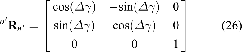
Firstly, the images n and o are rotated to $n^{\prime }$ and $o^{\prime }$ by ${ }^{n^{\prime }}{R}_n$ and ${ }^{o^{\prime }}{R}_o$ , respectively. Then, the following shows how to estimate the rotation matrix ${ }^{o^{\prime }}{R}_{n^{\prime }}$ of frame $F_{n^{\prime }}$ relative to frame $F_{o^{\prime }}$ based on the image moments.

Because the z axes of frames $F_{n^{\prime }}$ and $F_{o^{\prime }}$ are parallel to each other (see Figure 1(b)), ${ }^{o^{\prime }}{R}_{n^{\prime }}$ can be calculated by the image-centered moments. The rotation matrix ${ }^{o^{\prime }}{R}_{n^{\prime }}$ can be calculated by

${ }^{o^{\prime }}{R}_{n^{\prime }}=R_z\left(\Delta \gamma \right)$

19

where $\Delta \gamma {=}^{o^{\prime }}\gamma {-}^{n^{\prime }}\gamma$ . ${ }^{n^{\prime }}\gamma$ and ${ }^{o^{\prime }}\gamma$ are the orientation angles of the inertial principal axes of the target plane b on the images of cameras $n^{\prime }$ and $o^{\prime }$ . The orientation angles ${ }^{n^{\prime }}\gamma$ and ${ }^{o^{\prime }}\gamma$ can be calculated as (see the study of Horn ²⁴ for more details)

$\{\begin{array}{ll}\text{sin}\left(2\gamma \right)\hfill & =\frac{2c_{11}}{\sqrt{4c_{11}^2+{\left(c_{20}-c_{02}\right)}^2}}\hfill \\ \text{cos}\left(2\gamma \right)\hfill & =\frac{c_{20}-c_{02}}{\sqrt{c_{11}^2+{\left(c_{20}-c_{02}\right)}^2}}\hfill \end{array}$

20

where $c_{11}$ , $c_{20}$ , and $c_{02}$ are the second-order central moments and are defined by equation (7). It is well known that $\text{sin}\left(2\Delta \gamma \right)$ and $\text{cos}\left(2\Delta \gamma \right)$ can be expressed as

$\{\begin{array}{ll}\text{sin}\left(2\Delta \gamma \right)\hfill & =\text{sin}\left(2o^{\prime }\gamma \right)\text{cos}\left(2^{n^{\prime }}\gamma \right)-\text{cos}\left(2^{o^{\prime }}\gamma \right)\text{sin}\left(2^{n^{\prime }}\gamma \right)\hfill \\ \text{cos}\left(2\Delta \gamma \right)\hfill & =\text{cos}\left(2^{o^{\prime }}\gamma \right)\text{cos}\left(2^{n^{\prime }}\gamma \right)+\text{sin}\left(2^{o^{\prime }}\gamma \right)\text{sin}\left(2^{n^{\prime }}\gamma \right)\hfill \end{array}$

21

It is easy to get that

$\{\begin{array}{ll} \hfill & 2\text{sin}\left(\Delta \gamma \right)\text{cos}\left(\Delta \gamma \right)=\text{sin}\left(2\Delta \gamma \right)\hfill \\ \hfill & 2{{\displaystyle \text{cos}}}^2\left(\Delta \gamma \right)-1=\text{cos}\left(2\Delta \gamma \right)\hfill \end{array}$

22

Thus, the solution of equation (22) is obtained

$\Delta \gamma =\text{atan2}\left(\text{sin}\left(\Delta \gamma \right),\text{cos}\left(\Delta \gamma \right)\right)$

23

where

$\{\begin{array}{ll}\text{cos}\left(\Delta \gamma \right)\hfill & =\pm \sqrt{\frac{\text{cos}\left(2\Delta \gamma \right)+1}{2}}\hfill \\ \text{sin}\left(\Delta \gamma \right)\hfill & =\frac{\text{sin}\left(2\Delta \gamma \right)}{2\text{cos}\left(\Delta \gamma \right)}\hfill \end{array}$

There are two solutions calculated for $\Delta \gamma$ using equation (23), but only one solution set is correct. The following will explain how to choose the correct solution.

Selection of angles $\Delta {\gamma }_1$ and $\Delta {\gamma }_2$

This section will introduce the method for selecting the correct angle $\Delta \gamma$ by introducing the third-order moments.

The third-order moment equations are

$\{\begin{array}{ll}{\mu }_{30}=\hfill & {\Lambda }^3(A_{11}^3{\nu }_{30}+A_{12}^3{\nu }_{03}+3A_{11}^2{A}_{12}{\nu }_{21}\hfill \\ \hfill & +3A_{11}{A}_{12}^2{\nu }_{12})+3^{o^{\prime }}{O}_{n^{\prime }}{\mu }_{20}\hfill \\ \hfill & -3^{o^{\prime }}{O}_{n^{\prime }}^2{\mu }_{10}{+}^{o^{\prime }}{O}_{n^{\prime }}^3\hfill \\ {\mu }_{03}=\hfill & {\Lambda }^3(A_{21}^3{\nu }_{30}+A_{22}^3{\nu }_{03}+3A_{21}^2{A}_{22}{\nu }_{21}\hfill \\ \hfill & +3A_{21}{A}_{22}^2{\nu }_{12})+3^{o^{\prime }}{Q}_{n^{\prime }}{\mu }_{02}\hfill \\ \hfill & -3^{o^{\prime }}{Q}_{n^{\prime }}^2{\mu }_{01}{+}^{o^{\prime }}{Q}_{n^{\prime }}^3\hfill \\ {\mu }_{12}=\hfill & {\Lambda }^3[A_{11}{A}_{21}^2{\nu }_{30}+\left(A_{12}{A}_{21}^2+2A_{11}{A}_{22}{A}_{21}\right){\nu }_{21}\hfill \\ \hfill & +A_{12}{A}_{22}^2{\nu }_{03}+\left(A_{11}{A}_{22}^2+2A_{12}{A}_{21}{A}_{22}\right){\nu }_{12}]\hfill \\ \hfill & +2^{o^{\prime }}{Q}_{n^{\prime }}{\mu }_{11}{+}^{o^{\prime }}{O}_{n^{\prime }}{\mu }_{02}{-}^{o^{\prime }}{Q}_{n^{\prime }}^2{\mu }_{10}\hfill \\ \hfill & -2^{o^{\prime }}{O}_{n^{\prime }}{ }^{o^{\prime }}{Q}_{n^{\prime }}{\mu }_{01}{+}^{o^{\prime }}{O}_{n^{\prime }}{ }^{o^{\prime }}{Q}_{n^{\prime }}^2\hfill \\ {\mu }_{21}=\hfill & {\Lambda }^3[A_{11}^2{A}_{21}{\nu }_{30}+\left(A_{22}{A}_{11}^2+2A_{12}{A}_{21}{A}_{11}\right){\nu }_{21}\hfill \\ \hfill & +A_{12}^2{A}_{22}{\nu }_{03}+\left(A_{21}{A}_{12}^2+2A_{11}{A}_{22}{A}_{12}\right){\nu }_{12}]\hfill \\ \hfill & +2^{o^{\prime }}{O}_{n^{\prime }}{\mu }_{11}{+}^{o^{\prime }}{Q}_{n^{\prime }}{\mu }_{20}{-}^{o^{\prime }}{O}_{n^{\prime }}^2{\mu }_{01}\hfill \\ \hfill & -2^{o^{\prime }}{O}_{n^{\prime }}{ }^{o^{\prime }}{Q}_{n^{\prime }}{\mu }_{10}{+}^{o^{\prime }}{O}_{n^{\prime }}^2{ }^{o^{\prime }}{Q}_{n^{\prime }}\hfill \end{array}$

24

Substituting for ${ }^{o^{\prime }}{O}_{n^{\prime }}{,}^{o^{\prime }}{Q}_{n^{\prime }}$ using equation (12), we get

$\{\begin{array}{ll}{\overline{\mu }}_{30}\left(\Delta \gamma \right)=\hfill & {\Lambda }^3\left(K_{30}^a-K_{30}^b\right)-\Lambda K_{30}^c-K_{30}^d\hfill \\ {\overline{\mu }}_{03}\left(\Delta \gamma \right)=\hfill & {\Lambda }^3\left(K_{03}^a-K_{03}^b\right)-\Lambda K_{03}^c-K_{03}^d\hfill \\ {\overline{\mu }}_{12}\left(\Delta \gamma \right)=\hfill & {\Lambda }^3\left(K_{12}^a-K_{12}^b\right)-\Lambda K_{12}^c-K_{12}^d\hfill \\ {\overline{\mu }}_{21}\left(\Delta \gamma \right)=\hfill & {\Lambda }^3\left(K_{21}^a-K_{21}^b\right)-\Lambda K_{21}^c-K_{21}^d\hfill \end{array}$

25

where

$\{\begin{array}{ll}{K}_{30}^a=\hfill & A_{11}^3{\nu }_{30}+A_{12}^3{\nu }_{03}+3A_{11}^2{A}_{12}{\nu }_{21}+3A_{11}{A}_{12}^2{\nu }_{12}\hfill \\ K_{30}^b=\hfill & {\left(A_{11}{\nu }_{10}+A_{12}{\nu }_{01}\right)}^3\hfill \\ K_{30}^c=\hfill & 3\left(A_{11}{\nu }_{10}+A_{12}{\nu }_{01}\right)\left({\mu }_{20}-{\mu }_{10}^2\right)\hfill \\ K_{30}^d=\hfill & 2{\mu }_{10}^3-3{\mu }_{10}{\mu }_{20}\hfill \end{array}$

$\{\begin{array}{ll}{K}_{03}^a=\hfill & A_{21}^3{\nu }_{30}+A_{22}^3{\nu }_{03}+3A_{21}^2{A}_{22}{\nu }_{21}+3A_{21}{A}_{22}^2{\nu }_{12}\hfill \\ K_{03}^b=\hfill & {\left(A_{21}{\nu }_{10}+A_{22}{\nu }_{01}\right)}^3\hfill \\ K_{03}^c=\hfill & 3\left(A_{21}{\nu }_{10}+A_{22}{\nu }_{01}\right)\left({\mu }_{02}-{\mu }_{01}^2\right)\hfill \\ K_{03}^d=\hfill & 2{\mu }_{01}^3-3{\mu }_{01}{\mu }_{02}\hfill \end{array}$

$\{\begin{array}{ll}{K}_{12}^a=\hfill & A_{11}{A}_{21}^2{\nu }_{30}+\left(A_{12}{A}_{21}^2+2A_{11}{A}_{22}{A}_{21}\right){\nu }_{21}\hfill \\ \hfill & +A_{12}{A}_{22}^2{\nu }_{03}+\left(A_{11}{A}_{22}^2+2A_{12}{A}_{21}{A}_{22}\right){\nu }_{12}\hfill \\ K_{12}^b=\hfill & \left(A_{11}{\nu }_{10}+A_{12}{\nu }_{01}\right){\left(A_{21}{\nu }_{10}+A_{22}{\nu }_{01}\right)}^2\hfill \\ K_{12}^c=\hfill & \left(A_{11}{\nu }_{10}+A_{12}{\nu }_{01}\right)\left({\mu }_{02}-{\mu }_{01}^2\right)\hfill \\ \hfill & +2\left(A_{21}{\nu }_{10}+A_{22}{\nu }_{01}\right)\left({\mu }_{11}-{\mu }_{01}{\mu }_{10}\right)\hfill \\ K_{12}^d=\hfill & 2{\mu }_{10}{\mu }_{01}^2-2{\mu }_{11}{\mu }_{01}-{\mu }_{02}{\mu }_{10}\hfill \end{array}$

$\{\begin{array}{ll}{K}_{21}^a=\hfill & A_{11}^2{A}_{21}{\nu }_{30}+\left(A_{22}{A}_{11}^2+2A_{12}{A}_{21}{A}_{11}\right){\nu }_{21}\hfill \\ \hfill & +A_{12}^2{A}_{22}{\nu }_{03}+\left(A_{21}{A}_{12}^2+2A_{11}{A}_{22}{A}_{12}\right){\nu }_{12}\hfill \\ K_{21}^b=\hfill & {\left(A_{11}{\nu }_{10}+A_{12}{\nu }_{01}\right)}^2\left(A_{21}{\nu }_{10}+A_{22}{\nu }_{01}\right)\hfill \\ K_{21}^c=\hfill & 2\left(A_{11}{\nu }_{10}+A_{12}{\nu }_{01}\right)\left({\mu }_{11}-{\mu }_{01}{\mu }_{10}\right)\hfill \\ \hfill & +\left(A_{21}{\nu }_{10}+A_{22}{\nu }_{01}\right)\left({\mu }_{20}-{\mu }_{10}^2\right)\hfill \\ K_{21}^d=\hfill & 2{\mu }_{01}{\mu }_{10}^2-2{\mu }_{11}{\mu }_{01}-{\mu }_{20}{\mu }_{01}\mathrm{.}\hfill \end{array}$

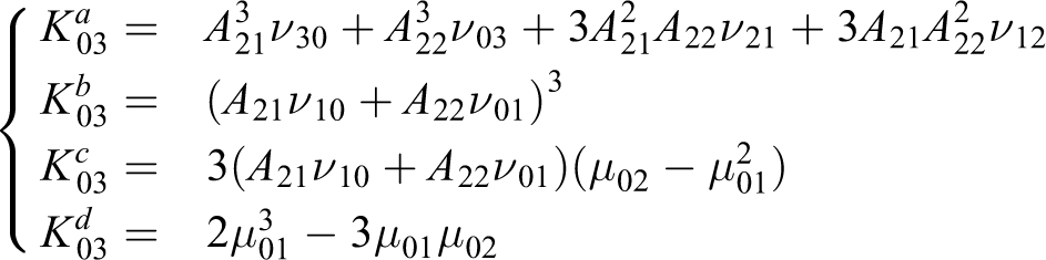
From equation (19), the rotation matrix ${ }^{o^{\prime }}{R}_{n^{\prime }}$ can be calculated as

${ }^{o^{\prime }}{R}_{n^{\prime }}=\left[\begin{array}{ccc}\text{cos}\left(\Delta \gamma \right)& -\text{sin}\left(\Delta \gamma \right)& 0\\ \text{sin}\left(\Delta \gamma \right)& \text{cos}\left(\Delta \gamma \right)& 0\\ 0& 0& 1\end{array}\right]$

26

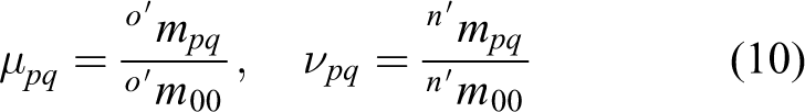
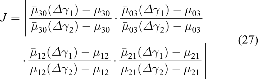
Therefore, it is easy to know that $A_{11}=\text{cos}\left(\Delta \gamma \right)$ , $A_{12}=-\text{sin}\left(\Delta \gamma \right)$ , $A_{21}=\text{sin}\left(\Delta \gamma \right)$ , and $A_{22}=\text{cos}\left(\Delta \gamma \right)$ . ${\overline{\mu }}_{pq}$ , ${\mu }_{pq}$ and ${\nu }_{pq}$ are calculated by equations (25) and (10), respectively. Theoretically, ${\overline{\mu }}_{pq}$ is the estimate of ${\mu }_{pq}$ . Therefore, if $\Delta \gamma$ is correct, then ${\overline{\mu }}_{03}\left(\Delta \gamma \right)={\mu }_{03}$ , ${\overline{\mu }}_{30}\left(\Delta \gamma \right)={\mu }_{30}$ , ${\overline{\mu }}_{12}\left(\Delta \gamma \right)={\mu }_{12}$ , and ${\overline{\mu }}_{21}\left(\Delta \gamma \right)={\mu }_{21}$ . To increase the robustness of the angle selection method, we define

$\begin{array}{l}J=|\frac{{\overline{\mu }}_{30}\left(\Delta {\gamma }_1\right)-{\mu }_{30}}{{\overline{\mu }}_{30}\left(\Delta {\gamma }_2\right)-{\mu }_{30}}\cdot \frac{{\overline{\mu }}_{03}\left(\Delta {\gamma }_1\right)-{\mu }_{03}}{{\overline{\mu }}_{03}\left(\Delta {\gamma }_2\right)-{\mu }_{03}}\hfill \\ \cdot \frac{{\overline{\mu }}_{12}\left(\Delta {\gamma }_1\right)-{\mu }_{12}}{{\overline{\mu }}_{12}\left(\Delta {\gamma }_2\right)-{\mu }_{12}}\cdot \frac{{\overline{\mu }}_{21}\left(\Delta {\gamma }_1\right)-{\mu }_{21}}{{\overline{\mu }}_{21}\left(\Delta {\gamma }_2\right)-{\mu }_{21}}|\hfill \end{array}$

27

If $\Delta {\gamma }_1$ is correct, then $J\to 0$ . Otherwise, $J\to \infty$ . So the positive coefficient $K_{\mu }$ is defined (usually $K_{\mu }=1$ can be taken). If $J>K_{\mu }$ is satisfied, $\Delta {\gamma }_2$ is the correct solution; otherwise, $\Delta {\gamma }_1$ is the correct solution.

Finally, the relative rotation matrix ${ }^o{R}_n$ of the two camera frames $F_n$ and $F_o$ can be calculated by equation (13), where ${ }^{o^{\prime }}{R}_o{,}^{o^{\prime }}{R}_{n^{\prime }}$ , and ${ }^{n^{\prime }}{R}_n$ are defined in equations (18), (19), and (14), respectively.

Estimate the translation vector of the two camera frames

This part will introduce the estimation method of the translation vector ${ }^o{t}_n$ in Figure 1(a).

From the camera frames $F_n$ and $F_o$ rotation introduced in the previous section, we can obtain

$\{\begin{array}{l}{ }^{n^{ }}p={\frac{{ }^{n^{\prime }}Z}{{ }^{n^{ }}Z}}^{n^{\prime }}{R}_{n^{ }}{ }^{{\text{T}n}^{\prime }}p\hfill \\ { }^{o^{ }}p={\frac{{ }^{o^{\prime }}Z}{{ }^{o^{ }}Z}}^{o^{\prime }}{R}_{o^{ }}{ }^{{\text{T}o}^{\prime }}p\hfill \end{array}$

28

where ${ }^{n^{\prime }}{R}_n$ and ${ }^{o^{\prime }}{R}_o$ are defined in equations (14) and (18), respectively, and ${ }^{n^{\prime }}Z$ and ${ }^{o^{\prime }}Z$ can be calculated as

$\{\begin{array}{ll}{ }^{n^{\prime }}Z\hfill & =\frac{1}{{ }^{n^{\prime }}C}\hfill \\ { }^{o^{\prime }}Z\hfill & =\frac{1}{{ }^{o^{\prime }}C}\hfill \end{array}$

where ${ }^{n^{\prime }}C$ and ${ }^{o^{\prime }}C$ are expressed as

$\{\begin{array}{ll}{ }^{n^{\prime }}C\hfill & {=||}^{n^{\prime }}{R}_n{ }^{n}N{||=||}^{n}N||\hfill \\ { }^{o^{\prime }}C\hfill & {=||}^{o^{\prime }}{R}_o{ }^{o}N{||=||}^{o}N||\hfill \end{array}$

Substituting for ${ }^{n}p$ , ${ }^{o}p$ , and ${ }^o{R}_n$ using equations (28) and (13), equation (3) can be converted to

${ }^{o^{\prime }}p={\frac{{ }^{n^{\prime }}Z}{{ }^{o^{\prime }}Z}}^{o^{\prime }}{R}_{n^{\prime }}{ }^{n^{\prime }}p+{\frac{1}{{ }^{o^{\prime }}Z}}^{o^{\prime }}{R}_o{ }^o{t}_n$

29

Because the imaging planes of the camera frames $F_{n^{\prime }}$ and $F_{o^{\prime }}$ are parallel, ${ }^{n^{\prime }}Z$ and ${ }^{o^{\prime }}Z$ are constant. According to equations (29) and (12), the relationship between the image moments of cameras $o^{\prime }$ and $n^{\prime }$ can be expressed as

${ }^{o^{\prime }}V={\frac{{ }^{n^{\prime }}Z}{{ }^{o^{\prime }}Z}}^{o^{\prime }}{R}_{n^{\prime }}{ }^{n^{\prime }}V+{\frac{1}{{ }^{o^{\prime }}Z}}^{o^{\prime }}{R}_o{ }^o{t}_n$

30

where ${ }^{o^{\prime }}V$ and ${ }^{n^{\prime }}V$ are defined as

${ }^{o^{\prime }}V=\left[\begin{array}{c}{\mu }_{10}\\ {\mu }_{01}\\ 1\end{array}\right],{}^{n^{\prime }}V=\left[\begin{array}{c}{\nu }_{10}\\ {\nu }_{01}\\ 1\end{array}\right]$

As a result, the translation vector ${ }^o{t}_n$ is obtained

${ }^o{t}_n{=}^{o^{\prime }}{R}_o^{\text{T}}\left({ }^{o^{\prime }}{Z}^{o^{\prime }}V{-}^{n^{\prime }}{Z}^{o^{\prime }}{R}_{n^{\prime }}{ }^{n^{\prime }}V\right)$

31

Therefore, the calculation method of the homogeneous transformation matrix has been completed.

Plane parameters estimation based on image moments

The homogeneous transformation matrix calculation method introduced in the third section needs to know the plane parameters in the frames $F_n$ and $F_o$ . In visual servo control, the latter is usually known, but the former is difficult to know. So we need to use the known information of image o and plane parameters ${ }^{o}N$ to estimate plane parameters ${ }^{n}N$ . The methods introduced in the studies of Chaumette ¹¹ and Chaumette et al. ²³ apply only to typical primitives. Therefore, the following will present a plane parameters estimate method, which is suitable for any pattern.

Generally, the plane parameters ${ }^{o}N$ are known, so we can calculate the rotation matrix ${ }^{o^{\prime }}{R}_o$ and get the rotated image $o^{\prime }$ . However, there are errors in the plane parameters ${ }^{\stackrel{\sim }{n}}N$ . Similarly, the rotation matrix ${ }^{\stackrel{\sim }{n}\text{'}}{R}_n$ and the rotated image $\stackrel{\sim }{n}\text{'}$ can be calculated (note if there is no error in ${ }^{\stackrel{\sim }{n}}N$ , $\stackrel{\sim }{n}\text{'}=n^{\prime }$ ). Theoretically, the 2D rotation, 2D translation, and scale invariant moments of images $o^{\prime }$ and $n^{\prime }$ are the same. So we can correct the plane parameters ${ }^{\stackrel{\sim }{n}}N$ according to these invariant moments.

We choose two moments $\varphi ={\left[{\varphi }_1,{\varphi }_2\right]}^{\text{T}}$ that are invariant to 2D rotation, 2D translation, and to scale ²⁵

$\{\begin{array}{ll}{\varphi }_1\hfill & =\frac{{\left(c_{50}+2c_{32}+c_{14}\right)}^2+{\left(c_{05}+2c_{23}+c_{41}\right)}^2}{{\left(c_{50}-10c_{32}+5c_{14}\right)}^2+{\left(c_{05}-10c_{23}+5c_{41}\right)}^2}\hfill \\ {\varphi }_2\hfill & =\frac{{\left(c_{50}-2c_{32}-3c_{14}\right)}^2+{\left(c_{05}-2c_{23}-3c_{41}\right)}^2}{{\left(c_{50}-10c_{32}+5c_{14}\right)}^2+{\left(c_{05}-10c_{23}+5c_{41}\right)}^2}\hfill \end{array}$

32

It is easy to know that ${ }^{n^{\prime }}\varphi {=}^{o^{\prime }}\varphi$ , so we can calculate ${ }^{n^{\prime }}\varphi$ from image $o^{\prime }$ . According to equation (9), the interaction matrix related to the invariant moments $\varphi$ has the following form

$\{\begin{array}{ll}{L}_{{\varphi }_1}\left(A,B,c_{pq}\right)\hfill & =\left[{\varphi }_{1_{vx}}{\varphi }_{1_{vy}}{\varphi }_{1_{vz}}{\varphi }_{1_{wx}}{\varphi }_{1_{wy}}0\right]\hfill \\ L_{{\varphi }_2}\left(A,B,c_{pq}\right)\hfill & =\left[{\varphi }_{2_{vx}}{\varphi }_{2_{vy}}{\varphi }_{2_{vz}}{\varphi }_{2_{wx}}{\varphi }_{2_{wy}}0\right]\hfill \end{array}$

33

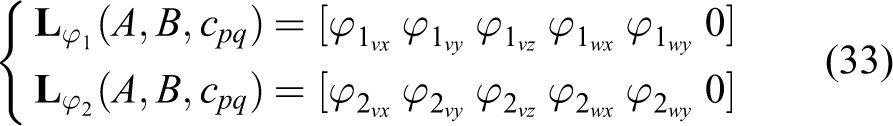
We want to rotate image $\stackrel{\sim }{n}\text{'}$ to image $n^{\prime }$ that is parallel to image $o^{\prime }$ , so ${\nu }_c=0$ and ${\omega }_c$ will be calculated. Therefore, we can get

$\dot{\varphi }=L_{\varphi }{\omega }_c$

34

where

$L_{\varphi }\left(c_{pq}\right)=\left[\begin{array}{ccc}{\varphi }_{1_{wx}}& {\varphi }_{1_{wy}}& 0\\ {\varphi }_{2_{wx}}& {\varphi }_{2_{wy}}& 0\end{array}\right]$

where $L_{\varphi }$ is not affected by plane parameters ${ }^{\stackrel{\sim }{n}}N$ with error. The invariant moments can be expressed as the Taylor expansion

${ }^{n^{\prime }}\varphi {=}^{\stackrel{\sim }{n}\text{'}}\varphi {+}^{\stackrel{\sim }{n}\text{'}}\dot{\varphi }\Delta t+O\left(\Delta t^2\right)$

35

Truncating the Taylor expansion at first order and substituting for ${ }^{\stackrel{\sim }{n}\text{'}}\dot{\varphi }$ using equations (34), we can approximate equation (35) as

${ }^{\stackrel{\sim }{n}\text{'}}{\omega }_c\Delta t{=}^{\stackrel{\sim }{n}\text{'}}{L}_{\varphi }^{†}\left({ }^{n^{\prime }}\varphi {-}^{\stackrel{\sim }{n}\text{'}}\varphi \right)$

36

Therefore, rotation matrix ${ }^{n^{\prime }}{R}_{\stackrel{\sim }{n}\text{'}}$ of the frame $F_{\stackrel{\sim }{n}\text{'}}$ relative to $F_{n^{\prime }}$ can be calculated as

${ }^{n^{\prime }}{R}_{\stackrel{\sim }{n}\text{'}}={\left({ }^{\stackrel{\sim }{n}\text{'}}{R}_{n^{\prime }}\right)}^{\text{T}}={\left(e^{{\left[{ }^{\stackrel{\sim }{n}\text{'}}{\omega }_c\right]}_{\times }\Delta t}\right)}^{\text{T}}$

37

where ${\left[{ }^{\stackrel{\sim }{n}\text{'}}{\omega }_c\right]}_{\times }$ is a $3\times 3$ skew-symmetric matrix representation of ${ }^{\stackrel{\sim }{n}\text{'}}{\omega }_c$ .

Now, we start to correct the initial plane parameters ${ }^{\stackrel{\sim }{n}}N$ . First, the image $\stackrel{\sim }{n}\text{'}$ will be rotated to $n^{\prime }$ by the rotation matrix ${ }^{n^{\prime }}{R}_{\stackrel{\sim }{n}\text{'}}$ . Noting that

$\sqrt{S}{=}^{o^{\prime }}Z\sqrt{{ }^{o^{\prime }}{m}_{00}}{=}^{n^{\prime }}Z\sqrt{{ }^{n^{\prime }}{m}_{00}}$

38

where S is the area of the object plane. Then, the plane parameter in the frame $F_{n^{\prime }}$ is ${ }^{n^{\prime }}N={\left[00{}^{n^{\prime }}C\right]}^{\text{T}}$ . According to equations (29) and (38), ${ }^{n^{\prime }}C$ can be expressed as

${ }^{n^{\prime }}C{=}^{o^{\prime }}C\sqrt{\frac{{ }^{n^{\prime }}{m}_{00}}{{ }^{o^{\prime }}{m}_{00}}}$

39

The final corrected plane parameters ${ }^{n}N$ are

${ }^{n}N={\left({ }^{n^{\prime }}{R}_{\stackrel{\sim }{n}\text{'}}{ }^{\stackrel{\sim }{n}\text{'}}{R}_n\right)}^{\text{T}}{ }^{n^{\prime }}N$

40

Plane parameter error $e_N$ can be calculated as $e_N={ }^{\stackrel{\sim }{n}}N{-}^n{N}^{*}$ , where the desired plane parameter ${ }^n{N}^{*}$ can be approximately expressed as ${ }^n{N}^{*}{\approx }^{n}N$ . Finally, we can design the correction scheme as

${\dot{e}}_N={ }^{\stackrel{\sim }{n}}\dot{N}=-{\lambda }_N{\widehat{e}}_N$

41

where ${\widehat{e}}_N={ }^{\stackrel{\sim }{n}}N{-}^{n}N$ .

PBVS and stability analysis

This section first introduces the PBVS control scheme, which is based on camera pose estimation described in the third section. Then, the stability of the method will be analyzed. This visual servoing scheme has been studied by Chaumette and Hutchinson. ²⁶ We briefly revisit the PBVS control scheme.

In this study, we can define the expected and current values of features $s^{*}=0$ and $s={\left[{ }^o{t}_n{\theta }^o{\omega }_n\right]}^{\text{T}}$ , in which ${ }^o{t}_n$ is a translation vector calculated using equation (31) and ${\theta }^o{\omega }_n$ gives the angle/axis parameterization for the rotation matrix ${ }^o{R}_n$ calculated by equation (13). Therefore, the vision-based control schemes minimize an error $e(t)$ , which is defined as

$e\left(t\right)=s-s^{*}={\left[{ }^o{t}_n{\theta }^o{\omega }_n\right]}^{\text{T}}$

The relationship between ${\dot{e}}_s$ and $v_c$ is given by

${\dot{e}}_s=\dot{s}=L_s{v}_c$

So the control scheme is obtained by

$v_c=-{\lambda }_s{\widehat{L}}_s^{-1}{e}_s$

42

where ${\widehat{L}}_s$ is an estimation of the interaction matrix $L_s$ related to $e_s$ and be calculated as

${\widehat{L}}_s=\left[\begin{array}{cc}{ }^o{R}_n& \mathbf{0}\\ \mathbf{0}& L_{{\theta }^o{\omega }_n}\end{array}\right]$

43

where $L_{{\theta }^o{\omega }_n}$ is given by ²⁷

$L_{{\theta }^o{\omega }_n}=I_3-\frac{\theta }{2}{\left[{ }^o{\omega }_n\right]}_{\times }+\left(1-\frac{\text{sinc}\left(\theta \right)}{{\text{sinc}}^2\left(\frac{\theta }{2}\right)}\right){\left[{ }^o{\omega }_n\right]}_{\times }^2$

where $\text{sinc}\left(x\right)$ is the sinus cardinal defined such that $x\text{sinc}\left(x\right)=\text{sin}\left(x\right)$ and $\text{sinc}\left(0\right)=1$ . According to equation (43), rotation and translation are decoupled, which allows us to obtain a simple control scheme

$\{\begin{array}{l}{\nu }_c=-{\lambda }_s^o{R}_n^{\text{T}}{ }^o{t}_n\hfill \\ {\omega }_c=-{\lambda }_s{\theta }^o{\omega }_n\hfill \end{array}$

44

Next, simply analyze the stability. Lyapunov function candidate is defined as

$V=\frac{1}{2}{e}_s^{\text{T}}{e}_s+\frac{1}{2}{e}_N^{\text{T}}{e}_N$

45

By deriving the Lyapunov function concerning time, equation (45) was transformed into

$\begin{array}{ll}\dot{V}\hfill & =e_s^{\text{T}}{\dot{e}}_s+e_N^{\text{T}}{\dot{e}}_N\hfill \\ \hfill & =-{\lambda }_s{e}_s^{\text{T}}{L}_s{\widehat{L}}_s^{-1}{e}_s-{\lambda }_N{e}_N^{\text{T}}{\widehat{e}}_N\hfill \end{array}$

46

If ${ }^n{N}^{*}\approx { }^{n}N$ is satisfied and the object plane is always in the camera field of view, then both

$-{\lambda }_s{e}_s^{\text{T}}{L}_s{\widehat{L}}_s^{-1}{e}_s\approx -{\lambda }_s{e}_s^{\text{T}}{e}_s<0$

and

$-{\lambda }_N{e}_N^{\text{T}}{\widehat{e}}_N\approx -{\lambda }_N{e}_N^{\text{T}}{e}_N<0$

will be guaranteed. So $\dot{V}<0$ , the system is asymptotically stable.

Simulation results

We evaluate the control scheme proposed in this article. Considering a vision sensor and a object plane as examples, the co-simulation was conducted on the MATLAB 2020b and CoppeliaSim 4.1 platforms. Some different patterns, that is, an “octopus,” a “whale,” and a “flame” (see Figures 2(a), 4(a), and 5(a)), were considered in the plane. The white noise with standard deviation $\sigma =0.1$ pixels is added to the image in the following simulations.

Simulation results using camera pose estimation

This part mainly verifies the effectiveness of the camera pose estimation method introduced in the third section, so we assume that plane parameters in the frame $F_n$ are known ( ${ }^{n}N={\left[-0.3716-0.05670.5307\right]}^{\text{T}}$ ). We consider the case where the image and object planes with the “octopus” pattern are nonparallel at the desired position ( ${ }^{o}N={\left[0.29860.15260.8273\right]}^{\text{T}}$ ). Figure 2(a) shows the green and red contours representing the desired and initial image contours, respectively. Then, PBVS scheme is used for camera control.

The obtained results are given in Figure 2. They show the good behavior of camera pose estimation and the control law. The translation component of the visual features is ${ }^o{t}_n$ , so the obtained camera trajectory is straight line (see Figure 2(b)). Despite the corresponding displacement is very large ( $t_x=0.1084\text{\hspace{0.17em} m},t_y=0.3403\text{\hspace{0.17em} m},t_z=-0.5524\text{\hspace{0.17em} m},\theta {\omega }_x=0.1370\text{\hspace{0.17em} rad},\theta {\omega }_y=0.4581\text{\hspace{0.17em} rad},\text{and}\theta {\omega }_z=-2.1889\text{\hspace{0.17em} rad}$ ), we can note in Figure 2(c) and (d) the decoupled and exponential decrease of the six combinations of the corresponding displacement and the six camera velocity components. Because the interaction matrix is decoupled, the corresponding displacement in Figure 2(c) all converge to less than ${10}^{-4}$ . Although noise is added, the pose estimation method proposed in this article is suitable when the image and object planes are nonparallel at the desired position.

Figure 2.

Results obtained using PBVS with known plane parameters: (a) “octopus” contour, (b) camera trajectory, (c) errors on pose, and (d) camera velocities. PBVS: position-based visual servoing.

In addition, the method proposed in this article is suitable for the case that $|\theta {\omega }_z|>\pi /2$ , but some methods based on image moments, that is, the methods proposed by Chaumette ¹¹ and Tahri and Chaumette, ¹² do not have this advantage. The following will design two simple situations to illustrate this problem.

The visual features in the method of Tahri and Chaumette ¹² are

$s={\left[x_n{y}_n{a}_n{\varphi }_1{\varphi }_2\alpha \right]}^{\text{T}}$

47

where ${\varphi }_1$ and ${\varphi }_2$ can be calculated by equation (32), and

$\{\begin{array}{ll}{x}_n\hfill & =a_n{x}_g\hfill \\ y_n\hfill & =a_n{y}_g\hfill \\ a_n\hfill & ={ }^{o}Z\sqrt{\frac{{ }^o{m}_{00}}{{ }^n{m}_{00}}}\hfill \\ \alpha \hfill & =\frac{1}{2}\text{arctan}\left(\frac{2c_{11}}{c_{20}-c_{02}}\right)\hfill \end{array}$

The “octopus” contour continues to be adopted, but $\theta {\omega }_x=0,\theta {\omega }_y=0$ (equivalent to $A=0,B=0$ ). One situation is $|\theta {\omega }_z|<\pi /2$ , the other is $|\theta {\omega }_z|>\pi /2$ (see Figure 3(a) and (b)). The obtained results are given in Figure 3. The method in this article can make the feature errors ( $e_s^{\alpha }$ ) and pose errors ( ${\left[e_{t_x}^{\alpha }{e}_{t_y}^{\alpha }{e}_{t_z}^{\alpha }{e}_{\theta {\omega }_x}^{\alpha }{e}_{\theta {\omega }_y}^{\alpha }{e}_{\theta {\omega }_z}^{\alpha }\right]}^{\text{T}}$ ) converge to less than ${10}^{-4}$ for both situations. However, the method proposed by Tahri and Chaumette ¹² is only suitable for case that $|\theta {\omega }_z|<\pi /2$ (see Figure 3(c) and (e)). For $|\theta {\omega }_z|>\pi /2$ , this method can only converge feature error ( $e_s^{\gamma }$ ) to less than ${10}^{-4}$ (see Figure 3(d)), while the pose error ( ${\left[e_{t_x}^{\gamma }{e}_{t_y}^{\gamma }{e}_{t_z}^{\gamma }{e}_{\theta {\omega }_x}^{\gamma }{e}_{\theta {\omega }_y}^{\gamma }{e}_{\theta {\omega }_z}^{\gamma }\right]}^{\text{T}}$ ) still has a large error, that is, $e_{\theta {\omega }_z}=-\pi$ (see Figure 3(f)). The reason is that the feature of the velocity ${\omega }_z$ is α, which is only available for $|\theta {\omega }_z|\in \left[-\pi /2,\pi /2\right]$ . Therefore, the calculation of ${ }^{o^{\prime }}{R}_{n^{\prime }}$ proposed in “The calculation of the rotation matrix ${ }^{o^{\prime }}{R}_{n^{\prime }}$ ” section has certain advantages for case that $|\theta {\omega }_z|>\pi /2$ .

Figure 3.

Results obtained using PBVS with known plane parameters: (a) “octopus” contour with $|\theta {\omega }_z|<\pi /2$ , (b) “octopus” contour with $|\theta {\omega }_z|>\pi /2$ , (c) errors on features with $|\theta {\omega }_z|<\pi /2$ , (d) errors on features with $|\theta {\omega }_z|>\pi /2$ , (e) errors on poses with $|\theta {\omega }_z|<\pi /2$ , and (f) errors on poses with $|\theta {\omega }_z|>\pi /2$ . PBVS: position-based visual servoing.

Simulation results using plane parameters estimation

This part mainly verifies the plane parameters estimation method introduced in the fourth section. We simulated a situation where a desired image and a object plane with the “whale” pattern are nonparallel at the desired position. ( ${ }^{o}N={\left[0.60160.21221.0419\right]}^{\text{T}}$ and ${ }^{n}N={\left[-0.3716-0.05670.5307\right]}^{\text{T}}$ ). Twenty-seven percent errors are randomly added to ${ }^{n}N$ to obtain plane parameters ${ }^{\stackrel{\sim }{n}}N={\left[-0.4617-0.07750.6778\right]}^{\text{T}}$ . Note that ${ }^{n}N$ is unknown, but ${ }^{\stackrel{\sim }{n}}N$ is known. Figure 4(a) shows the green and red contours representing the desired and initial image contours, respectively. The PBVS schemes with and without plane parameters estimation are used to control the cameras, respectively.

The obtained results are given in Figure 4. The camera trajectories controlled by the PBVS schemes with and without plane parameters estimation are shown in Figure 4(b) . Due to the early correction of plane parameter errors (Figure 4(c)), the trajectory obtained by the former method is slightly different from the straight-line trajectory in Figure 2(b). It is easy to see that the plane parameter errors of the former method ( ${\left[{ }^n{e}_A{}^n{e}_B{}^n{e}_C\right]}^{\text{T}}$ ) quickly converge to ${10}^{-4}$ , while the plane parameter errors of the latter method ( ${\left[{ }^{\stackrel{\sim }{n}}{e}_A{}^{\stackrel{\sim }{n}}{e}_B{}^{\stackrel{\sim }{n}}{e}_C\right]}^{\text{T}}$ ) still have a large error in Figure 4(c). Despite the corresponding displacement is large ( $t_x=-0.9133\text{\hspace{0.17em} m},t_y=-0.7534\text{\hspace{0.17em} m},t_z=-0.1625\text{\hspace{0.17em} m},\theta {\omega }_x=-0.2980\text{\hspace{0.17em} rad},\theta {\omega }_y=1.0479\text{\hspace{0.17em} rad},\text{and \hspace{0.17em}}\theta {\omega }_z=1.1873\text{\hspace{0.17em} rad}$ ), the pose errors obtained by the former method still all converge to less than ${10}^{-4}$ , but the pose errors ( ${\left[e_{t_x}^{\beta }{e}_{t_y}^{\beta }{e}_{t_z}^{\beta }{e}_{\theta {\omega }_x}^{\beta }{e}_{\theta {\omega }_y}^{\beta }{e}_{\theta {\omega }_z}^{\beta }\right]}^{\text{T}}$ ) obtained by the latter cannot converge to a small value (see Figure 4(d)). The PBVS scheme shows camera velocities (see Figure 4(e) and (f)). There is no oscillation for any component of the camera velocity in both methods.

Figure 4.

Results obtained using PBVS with errored plane parameters: (a) “whale” contour, (b) camera trajectories, (c) errors on plane parameters, (d) errors on pose, (e) camera velocities with plane parameters estimation, and (f) camera velocities without plane parameters estimation. PBVS: position-based visual servoing.

As a result, the plane parameters estimation method proposed in this article can effectively eliminate the parameter error, and satisfactory results are obtained in PBVS scheme.

Simulation results compared to the classical method

This part will show the comparison results between the method proposed in this article and the classical method proposed by Tahri and Chaumette. ¹² The latter’s visual features are expressed as equation (47) and the interaction matrix is

${\widehat{L}}_s=\frac{1}{2}\left(L_{s^{*}}+L_s\right)$

48

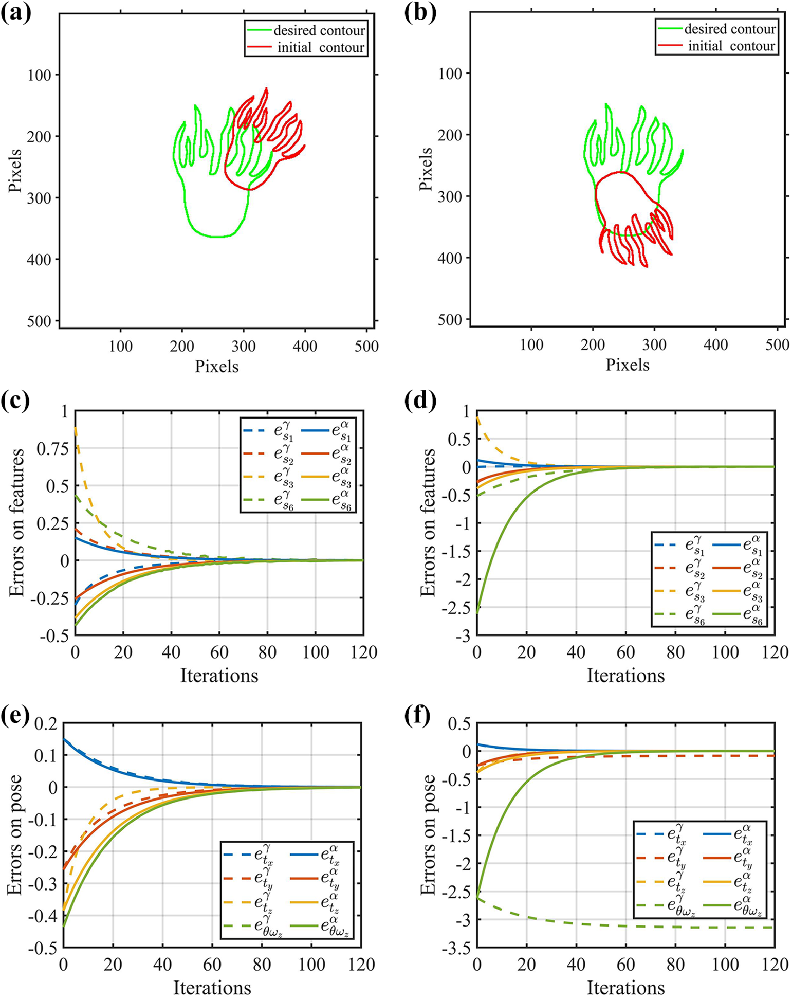
which largely improves the system behavior. ²⁸ The former’s interaction matrix is calculated by equation (43). We consider the case where the image and object planes with the “frame” pattern (see Figure 5(a)) are parallel at the desired position ( ${ }^{o}N={\left[001.1765\right]}^{\text{T}}$ and ${ }^{n}N={\left[-0.0083-0.29410.5290\right]}^{\text{T}}$ ). The corresponding displacement is $t_x=-1.0735\text{\hspace{0.17em} m},t_y=-0.4274\text{\hspace{0.17em} m},t_z=-0.8021\text{\hspace{0.17em} m},\theta {\omega }_x=-0.4925\text{\hspace{0.17em} rad},\theta {\omega }_y=0.1439\text{\hspace{0.17em} rad},\text{\hspace{0.17em} and \hspace{0.17em}}\theta {\omega }_z=-0.5007\text{\hspace{0.17em} rad}$ .

Firstly, we assume that the planar parameter ${ }^{n}N$ is known, and then use these two methods for visual servo control, respectively. The obtained results are shown in Figure 5.

Figure 5.

Results obtained using two methods with known plane parameters: (a) “frame” contour, (b) camera trajectory, (c) errors on features using classical method, (d) errors on features using our method, (e) errors on pose using classical method, (f) errors on pose using our method, (g) camera velocities using classical method, and (h) camera velocities using our method.

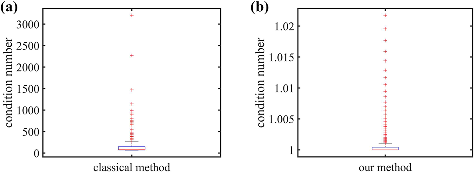
The camera trajectories controlled by the two methods are showed in Figure 5(b). Because our method adopts PBVS control scheme, the camera trajectory is a straight line; while the classical method adopts the IBVS control scheme, so the camera trajectory is a curve. The two methods can not only make the feature errors converge to ${10}^{-4}$ (see Figure 5(c) and (d)) but also make the pose errors converge to ${10}^{-4}$ (see Figure 5(e) and (f)). However, the camera velocities controlled by our method is more stable than the camera velocities controlled by the classical method (see Figure 5(g) and (h)). The result is that the interaction matrix computed by our method has a better condition number than the classical method. Because the former has a completely decoupled interaction matrix (equation (43)). The boxplots of condition numbers of interaction matrices obtained by two methods with known plane parameters are shown in Figure 6. The maximum, minimum, and mean values of the condition numbers calculated by the classical method are $3206.2393$ , $65.1757$ , and $209.3060$ , respectively. However, the maximum, minimum, and mean values of the condition numbers calculated by the our method are $1.0217$ , $1.000000$ , and $1.0014$ , respectively. Therefore, the method proposed in this article has obvious advantages over the classical method when the planar parameter ${ }^{n}N$ is known.

Figure 6.

The boxplots of condition numbers of interaction matrices obtained by two methods with known plane parameters: (a) classical method and (b) our method.

Finally, $30\%$ errors are randomly added to ${ }^{n}N$ to obtain plane parameters ${ }^{\stackrel{\sim }{n}}N={\left[-0.0116-0.18600.3650\right]}^{\text{T}}$ . Then, the two methods are respectively used for visual servo control. The obtained results are shown in Figure 7.

Figure 7.

Results obtained using two methods with errored plane parameters: (a) camera trajectory, (b) errors on plane parameters, (c) errors on features using classical method, (d) errors on features using our method, (e) errors on pose using classical method, (f) errors on pose using our method, (g) camera velocities using classical method, and (h) camera velocities using our method.

The camera trajectories controlled by the two methods are shown in Figure 7(a). Although there are errors in plane parameters, both methods can converge the visual features to ${10}^{-4}$ (see Figure 7(c) and (d)). However, our method can also converge the pose error to ${10}^{-4}$ , while the classical method can only converge to ${10}^{-2}$ (see Figure 7(e) and (f)). This is because the former method has plane parameter estimation and quickly converges the plane parameter errors to ${10}^{-4}$ , but the latter method does not have this advantage (see Figure 7(b)). It can be seen from Figure 7(g) and (h) that the camera velocities calculated by the method proposed in this article are still more stable than the camera velocities calculated by the classical method. The boxplots of condition numbers of interaction matrices obtained by the two methods with errored plane parameters are shown in Figure 8. The maximum, minimum, and mean values of the condition numbers calculated by the classical method are $2244.6194$ , $65.6998$ , and $130.4685$ , respectively. However, the maximum, minimum, and mean values of the condition numbers calculated by our method are $1.0214$ , $1.0000$ , and $1.0015$ , respectively. The latter is significantly smaller than the former. Therefore, the method proposed in this article still has obvious advantages over the classical method when the planar parameter ${ }^{\stackrel{\sim }{n}}N$ is errored.

Figure 8.

The boxplots of condition numbers of interaction matrices obtained by two methods with errored plane parameters: (a) classical method and (b) our method.

Conclusion

This study proposes two new estimation methods based on image moments, which are used to estimate camera pose and plane parameters, respectively. The former method, which is a closed-form solution, directly estimates the relative pose of the initial camera and the desired camera, not the pose of the camera relative to the object plane. The latter method uses the 2D rotation, 2D translation, and scale invariant moments to estimate the plane parameters. From both estimation methods, the article employs a PBVS scheme for the object plane. The simulation results have validated our approaches. One advantage of the two estimation methods is that they do not require image processing such as features extraction, matching, and tracking, the other is that the PBVS scheme is suitable for the case that $|\theta {\omega }_z|>\pi /2$ . In addition, the condition number of the interaction matrix calculated by the method proposed in this article is very small, which is very important for visual servo control. However, some particular configurations can make the object plane leave the camera field of view, which will affect the stability of visual servoing control. Future work will be devoted to designing a visual servoing scheme that increases the stability and prefer better decoupling of the interaction matrix.