Sage Journals: Discover world-class research

Abstract

In this article we present a novel mechanical design of a robot leg that possesses active and variable passive compliance properties. The hip and knee joints provide active compliance, while the variable passive compliance comes from the spiral foot spring, mounted on the ankle joint, which changes its stiffness by rotating and changing contact angle with the ground. The stiffness of the foot for various contact angles was identified experimentally by using the strength tester measurement system. The method for damping coefficient identification, based on the observation of energy losses during the stance phase of leg hopping motion, is described and used to obtain the foot damping model. The adaptation of spiral foot stiffness to varying ground stiffness is achieved by extracting a leg contact time from a feedback signal provided by a flex sensor mounted on the foot. The experiments on a single leg and quadruped platforms have confirmed that the presented spiral foot design provides stiffness adaptability, partial recovery of the energy from the previous hop and restriction of stance contact time, which are all necessary conditions to obtain more efficient quadruped locomotion.

Keywords

Passive Variable Compliance Quadruped Locomotion Adaptive Stiffness Control

1. Introduction

The extensive observations of the nature have revealed that complex high degree of freedom legged locomotion systems can be described by a reduced-order dynamics model called SLIP (The Spring Loaded Inverted Pendulum)[1 –3]. The simplified model consists of one body equivalent mass M at the top of a single linear spring with stiffnes k_leg, as shown in Figure 1. The motion represented by the SLIP model is characterized by two phases: flight phase and stance phase. Flight phase, during which the whole system is off the ground, ends when the leg touches down with a certain velocity v₀ and touchdown angle Θ. The result is the accumulation of potential elastic energy in the spring lasting until the end of spring compression [4]. At this point the leg spring stiffness k_leg can be calculated as the ratio of ground reaction force F_g and spring contraction ΔL:

Figure 1.

The SLIP model behaviour

k_{l e g} = \frac{F_{g}}{Δ L}

(1)

At the beginning of another flight phase, the portion of potential elastic energy stored in the spring assumes back a kinetic form represented by a take-off velocity v₁. The value of v₁ is determined by initial values of v₀, Θ, M and k_leg. Due to inevitable energy loss caused by leg damping c_leg, some energy must be added to the system so that uniform and continuous motion is maintained.

1.1 The role of leg stiffness in locomotion

The stiffness is particularly important in two aspects of legged locomotion which include work output and gait control [5, 6]. The locomotion speed is determined by a stride frequency, a number of hops or steps made in a period of time, and also by a stride length which is defined as a distance covered with each hop or step.

The same locomotion speed value can be achieved by combining different stride frequencies and lengths. If the stride length is constant, higher speed demands higher stride frequency which requires stiffer legs [7, 8]. On the other hand, the increase of speed by increasing the stride length and keeping the stride frequency constant does not demand the change of the stiffness [9, 10]. Namely, the increase of stride length reduces the touchdown angle Θ, which ultimately results in a reduced vertical travel of the center of mass ΔL while keeping the leg stiffness constant.

In [7] it is shown that the stride frequency selected by any running or hopping animal optimizes the energy cost of locomotion. The human Achilles tendon absorbs up to 35% of the total mechanical energy during each stride while the horse tendon conserves as much as 40% of mechanical work for trotting and galloping [11].

Locomotion at stride frequencies above optimal demands a stiffer leg which dissipates higher energy in collision with the ground, requires faster and energy demanding muscular activity and introduces high stresses. Too low leg stiffness at lower stride frequencies increases the stance time, which is energetically expensive because the actuators must hold a body mass against the gravity for a longer period of time.

Numerous studies have shown an important link between the leg stiffness and ground stiffness values. In [12] it is shown that a vertical mass displacement ΔL remains constant in spite of immense changes in the ground stiffness k_g (see Figure 1). In other words, while they are running on stiffness-varying surfaces (varying k_g), humans tend to adapt the stiffness of their legs k_leg so that the effective stiffness in vertical direction remains constant. The authors’ final conclusion is that kinematic variables such as stride frequency and ground contact time T_c remain unchanged during hopping or running on stiffness-varying surfaces in order to minimize the metabolic cost of locomotion.

Regarding the gait control, one can conclude that natural leg stiffness compensates changes in ground stiffness in order to maintain the stride frequency constant at the desired energy optimal value. Additionally, the changes in locomotion speed influence the leg stiffness only if the stride frequency is changing.

1.2 Compliance in robot leg design

Compliance in robotics is known and researched [6, 13]. It ensures that the interaction between the robot and its surroundings during task execution conforms to environment characteristics and safety requirements without compromising the robot operation. The robot leg compliance makes it possible for the robot to filter the unexpected ground force impulses, but most importantly improves the locomotion stability on surfaces with variable geometry and stiffness. Depending on the robot leg mechanical design and control, three types of compliance exist: the fully passive (fixed and variable), the fully active and the hybrid which combines both active and passive compliance.

The fixed passive compliance is achieved by using a mechanical spring with stiffness k_p and damping c_p. The biggest advantage of using a mechanical spring is elastic energy absorption in the compression phase, which is partially converted to kinetic energy during the extension phase. The obtained output kinetic energy is dominantly reduced due to losses caused by damping c_p and can be recovered through actuation. For example, the leg design of the experimental quadruped platform Scout II presented in [14] has two DOF, the active hip rotation joint and the prismatic passive spring. The robot bouncing stride frequency is limited due to the fixed spring parameters but the specific resistance of locomotion [15] shows that the robot successfully reuses elastic potential energy. The one-legged hopping robot ARL-Monopod II presented in [16] reuses spring energy to achieve the smallest specific locomotion resistance. The bow leg planar hopping robot is presented in [17]. The leg design is based on a curved leaf spring which reduces the need for additional actuation energy. The use of the fixed passive compliance ensures elastic energy absorption but the robot locomotion has no ability to adapt to different ground stiffness.

The active compliance requires torque control of robot actuators to provide a spring-like dynamic behaviour. A fully torque-controlled hydraulically actuated quadruped (HyQ) robot is presented in [18]. The highly dynamic active compliance is achieved to ensure fast locomotion over rough terrain. A compliant quadruped robot StarlETH uses brushless DC motors to achieve active compliance [19]. Additional mechanical springs are included into the leg structure in order to recover some energy and ensure certain passive compliance.

The biggest drawback of fully active compliance is the inability to absorb and restore energy. The only solution which mimics the compliance in the real world is the one that uses variable passive compliance leg design. To the best of authors’ knowledge, the earliest known research which analyses elastic storage mechanisms is the MIT technical report that explores active balance for the dynamic legged systems presented in [20]. The authors analyse the property of the material to store the energy starting from steel in tension towards compressed gas. The hydraulic-pneumatic telescoping leg is presented which contains an air chamber with controllable air pressure to simulate a variable spring. The latest variable compliance mechanisms rely on relatively complex designs which include a combination of non-linear springs in combination with at least one actuator in order to control the compliance of the entire mechanical system. An actuator with mechanical adjustable series compliance (AMASC) is depicted in [21]. The nonlinear spring behaviour is formed by a set of spiral pulleys which deform the two fibreglass springs. The compliance and the equilibrium position can be controlled independently by using dedicated motors. Similar mechanically complex approaches can be found in [22, 23].

The principle adopted for the presented foot design has similarities to the RHex hexapod C-leg solutions [24, 25]. The RHex C-leg is designed as a compliant C-shaped beam which is rotated by a single actuator. During the rotation the C-leg produces vertical and longitudinal forces to the body which allows the efficient RHex locomotion through “flowable ground” such as grass, mud or sand [26]. The design of a C-shaped multi-directional variable stiffness leg for RHex is described in [27, 28]. The leg stiffness can be varied with an actuated slider position. As the leg rolls during the stance phase, its stiffness additionally changes depending on a rolling contact point position whose influence, according to the authors, is not significant and can be additionally compensated by optimization.

All presented robot leg designs have the ability to control compliance but they lack information on how to detect the ground stiffness, which is needed as feedback for stable gait control on stiffness-varying surfaces. The authors in [29] conclude that human runners completely adjust the leg stiffness during the first step on the unknown surface only if they knew in advance that the change would happen and already had experience about the ground stiffness from the past. Unexpected ground stiffness transition could lead to disruptions that might cause losing the balance.

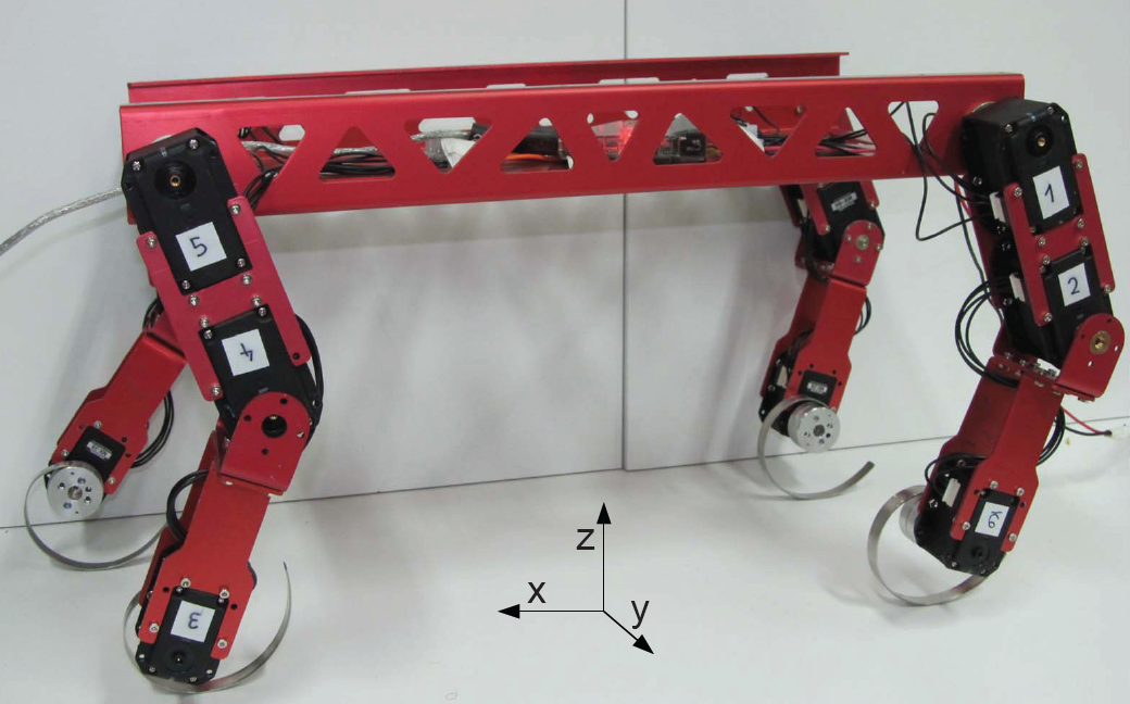
This research suggests that a robot could prepare itself in advance for the stiffness transition by using, for example, the image processing feedback, and then during the transition, it could use a ground stiffness feedback from the leg for adaptation of leg stiffness if possible. For this purpose a novel design of a quadruped robot with legs having their feet in the form of a spiral spring attached to the rotary shaft of the ankle is proposed (see Figure 2). The fact that the spiral spring can rotate and change the contact angle with the ground extends the variable passive property to the leg in a whole and thus enables direct stiffness control during robot motion. This feature should allow the robot to walk, run and jump with higher energy efficiency than the concurrent simpler quadruped robot designs. The first prototype of the envisioned quadruped robot, called Dynarobin, having oval feet firmly attached to the legs was presented in [30].

Figure 2.

Dynarobin - a compliant quadruped robot design

The remainder of article is organized in the following way. In section 2 a compliant leg design is presented. Also, foot spring stiffness is experimentally identified using a strength tester measurement system. A method for damping coefficient identification, based on the observation of energy losses during the stance phase of hopping, is described. The analytic solution is derived from observing the mathematical model of a bouncing ping-pong ball. In section 3 a vision tracking system is used to measure the hopping leg position and velocity, which were used to calculate the damping coefficient. The foot contact angle adaptation algorithm, based on a contact time feedback measured by a flex sensor, is presented and tested on a single leg experimental platform. The final experiment evaluates the possibilities and requirements of a foot used on the quadruped robot like Dynarobin in section 4. We conclude the article with final remarks in section 5.

2. Novel Compliant Leg Design

A planar 3-DOF robot leg design with active and variable passive compliance properties, which can be easily upgraded to a 4-DOF leg by adding a lateral hip joint, is shown in Figure 3. The leg consists of three revolute joints (i.e. hip, knee, and ankle), two rigid links (thigh and lower leg) and a foot having the form of a rotary head with a flexible spiral shaped beam (see Figure 4). The robot leg mass M contains masses of servo motors, links and other present elements. The hip and knee joints, actuated with Dynamixel MX-64 motors, control the (x, z) position of the leg, but through torque control they also provide active leg compliance. The ankle joint, which rotates a spiral foot, is actuated by the Dynamixel MX-28 motor.

Figure 3.

The leg design with a spiral foot attached to the ankle

Figure 4.

The spiral foot CAD model

Biological equivalents to torque controlled robot actuators are muscles, which connected tightly with bones and tendons, enable both actuation and active compliance during locomotion. Muscles can be modelled in a simplified way as springs with variable stiffness coefficient k_a, variable damping coefficient c_a and controllable initial length L_a0. The same simplified model can be directly applied to a robot leg, as depicted in Figure 3.

In order to measure the foot spring contraction during a ground contact phase, a low cost flex sensor is attached to the spiral foot. Measuring of contraction duration can give not only the information about the beginning of the stance phase, but also can serve as a basis for rudimentary approximation of the ground stiffness coefficient k_g. This information can serve as a feedback to the leg stiffness control algorithm.

The aim of introducing the revolute flexible foot is to get closer to the functionality of a real tendon. We can model it as an additional spring with a stiffness coefficient k_s, damping coefficient c_s and initial length L_s0. By rotating the foot during the flight phase, fast and reliable control of the contact point between the foot and the ground becomes possible, which directly affects (changes) k_s, c_s and L_s0, turning them into controllable parameters. The active hip/knee compliance and adjustable passive foot compliance yield the total leg compliance parameters k_L and c_L. By knowing the configuration of terrain (here we consider only flat stiffness-varying terrains) and by controlling the point of foot contact with the ground, we provide basic conditions for implementation of robot stiffness control.

A spiral foot (its CAD model is depicted in Figure 4) consists of a stainless steel based spiral-shaped spring connected to the ankle motor shaft through an aluminium head with a total mass of M_s. The foot passive compliance properties depend on mechanical characteristics of a spiral-shaped spring: used material, thickness A, width B and radius r(α). The radius r(α) represents the spring relative distance to the central rotational axis e with respect to angle α. The angle α can be also represented as a contact angle in relation to the flat ground surface depicted in Figure 5. The lowest foot stiffness is expected for α = 0°, ascending thereafter non-linearly to its maximum at approximately α = 225°.

Figure 5.

The contact angle α

The mechanical foot design is adapted to the robot prototype size and weight and all spring identification and analysis is performed accordingly (see robot and foot parameters in Table 1). Used materials, curvature, width and thickness define values of foot stiffness k_s(α) and damping c_s(α). The curvature radius of the spring (foot length) is in the range from 0.02 m to 0.06 m (10% to 27% of the leg length) which satisfies the cat-alike natural three-segmented limb ratio [31]. The foot spring width (0.01 m) and thickness (0.001 m) are conditioned by a single leg load value around M_l = 0.58 kg and by the requirement that the largest displacement of the foot head should not exceed the maximally allowed contraction of the foot at the contact angle α = 0°, i.e. when foot stiffness k_s is the lowest. More detailed analysis of influence of mechanical design characteristics on k_s(α) and c_s(α) demands deeper simulation and experimental analysis by using the Finite Element Analysis method as shown in [32], which is beyond the scope of this article.

Table 1.

Dynarobin and spiral foot design characteristics

Dynarobin mass:	3 kg
Dynarobin size(LxHxW):	0.42 m × 0.19 m × 0.23 m
Dynarobin leg length:	0.22 m
Spiral foot material:	17–4 PH stainless steel
Spiral foot curvature radius:	r(α) = (0.06 – 0.0015 · α) [m]
Spiral foot thickness:	0.001 [m]
Spiral foot width:	0.01 [m]

3. Identification of Spiral Foot Compliance Parameters

The spiral foot stiffness identification was performed by using a strength tester TensoLab 3000 [33] measurement system shown in Figure 6. The experimental platform consists of a measuring load cell attached to a base plate which can be vertically translated. The other part of the load cell is connected to the foot which is rotated by control of the ankle joint servo motor. During one measurement the foot head undergoes a series of angular displacements equal to 22.5° starting from α = 0° to α = 180°. For each angle the foot is positioned above the ground and then vertically translated with a speed of 0.05 m/min.

Figure 6.

The spiral foot identification process

Force measurement starts at foot touchdown (Δ = 0 m) and ends either when the maximum displacement Δ = 0.02 m or maximum force F = 55 N are observed. In total three measurements for each observed angle were conducted (see Figure 7). The family of average curves F = f(Δ) for α = (0, 22.5,.., 180) were then approximated with 2nd-degree or 1st-degree polynomials as depicted in Figure 8 and Table 2.

Figure 7.

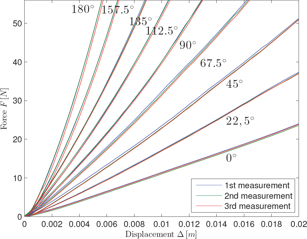
Force measurement depending on α (three measurements for each angle repeated)

Figure 8.

Force measurement depending on displacement Δ, first and second-order approximation

Table 2.

Spiral foot contact force - first and second degree approximation for different α[°]

α [°]	F(Δ)[N] 2^nd-degree approx.	MSE	F(Δ)[N]1^st-degree approx.	MSE
0	= 9479.4Δ² + 1039.8Δ	0.0505	= 1145.4Δ	0.17
22.5	= 2458.6Δ² + 1458.5Δ	0.10	= 1732.3Δ	0.15
45	= 2608.7Δ² + 2082.9Δ	0.0747	= 2432.1Δ	0.14
67.5	= 4856.7Δ² + 2713.6Δ	0.0900	= 3254.4Δ	0.51
90	= 1058.7Δ² + 2940.5Δ	0.045	= 3981.3Δ	0.94
112.5	= 1673.9Δ² + 3581.2Δ	0.0838	= 4960.5Δ	2.02
135	= 2365.8Δ² + 4139.0Δ	0.0114	= 6208.8Δ	2.74
157.5	= 5968.0Δ² + 4234.2Δ	0.1163	= 6885.4Δ	3.54
180	= 9141.3Δ² + 9141.3Δ	0.0990	= 8600.7Δ	3.30

Although the second-degree polynomial best fit the stiffness function (smaller MSE), the linear approximation k_s for each angle was chosen as it provides adequate accuracy and simplicity and is therefore going to be used in the foot damping coefficient identification (see Table 3). Finally, the second-degree polynomial approximation of stiffness k_s as a function of foot angle α[°] is shown graphically in Figure 9 and represented analytically as:

k_{s} (α) = 0.1 \cdot α^{2} + 21.4 \cdot α + 1208.1

(2)

Figure 9.

Second-order approximation of stiffness k_s as a function of spiral foot angle α[°]. The red dots represent the measured k_s values from Table 3.

Table 3.

Spiral foot stiffness - first-degree approximation for different α[°]

α [°]	k_s [N/m]	α [°]	k_s [N/m]
0	1145.4	112.5	4960.5
22.5	1732.3	135	6208.8
45	2432.1	157.5	6885.4
67.5	3254.4	180	8600.7
90	3981.3

In addition to the stiffness coefficient k_s, the spiral foot contains damping coefficient c_s which causes energy losses during the stance phase. In order to analytically calculate the energy losses, we assume that hip and knee actuators are locked (k_a → ∞), and the entire leg is observed as a simple mass-spring-damper model with total mass M_L = M + M_s, stiffness k_s and damping c_s. The ground stiffness is assumed to be very stiff (k_g → ∞) and without damping (c_g = 0 Ns/m) (see Figure 10).

Figure 10.

A mass-spring damper model with a mass M_L and stiffness k_s and damping c_s

At the initial stage of the jump, the leg is at height h₀ with initial speed υ = ||v|| = 0. The flight phase ends at height z = L_s0 which is the initial spring length. The initial contact speed is υ = υ₀ = ||v₀||. The spring compresses maximally when the speed drops to zero. The second part of the stance phase is the acceleration towards the speed υ = υ₁ = ||v₁||. The stance phase ends when the position of the mass M_L exceeds the initial spring length L_s0.

The final height h₁ depends on the velocity υ₁ obtained at the end of the stance phase. The energy losses can be observed as a difference between the kinetic energy calculated at υ₀ and υ₁. Since it is easier to measure the height difference Δh = h₁ – h₀ rather than the speed difference Δυ = υ₁ – υ₀, it is easier to observe the difference in the potential energy.

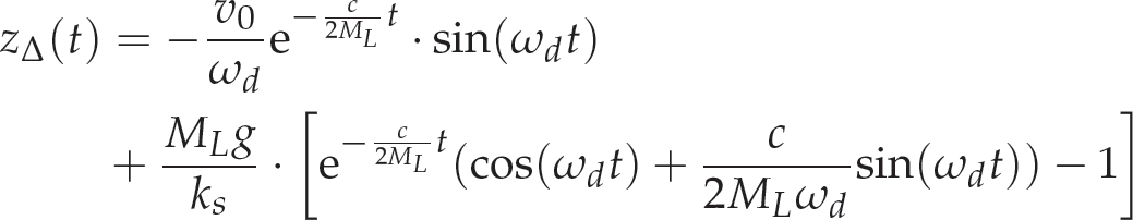
The analytic solution to the energy losses problem is inspired by the work in [34] where the mass-spring-damper model of a bouncing ping-pong ball has been analysed. The motion of a leg is observed in the translated coordinate frame (x, zΔ) which yields:

M_{L} {\ddot{z}}_{Δ} + c_{s} {\dot{z}}_{Δ} + k_{s} z_{Δ} = - M_{L} g_{0}

(3)

where Z_Δ(t) = z(t) – L_s0 and g₀ = 9.81m/s² represents the gravity. Using the initial conditions of z_Δ(0) = 0 and υ(0) = –υ₀, where υ₀ is the velocity of mass M_L at the initial contact, the analytical solution yields:

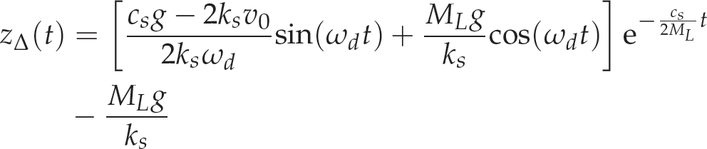
\begin{array}{l} z_{Δ} (t) & = [\frac{c_{s} g - 2 k_{s} v_{0}}{2 k_{s} ω_{d}} \sin (ω_{d} t) + \frac{M_{L} g}{k_{s}} \cos (ω_{d} t)] e^{- \frac{c_{s}}{2 M_{L}} t} \\ - \frac{M_{L} g}{k_{s}} \end{array}

(4)

where

ω_{d} = \frac{1}{2 M_{L}} \sqrt{4 k_{s} M_{L} - c_{s}^{2}}

(5)

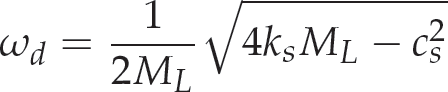
The total hopping period consists of the stance contact time T_c and the flight time T_f. T_c can be obtained from (4) by finding the first solution to the equation z_Δ(0) = 0. In order to solve it analytically, the equation (4) is rearranged as:

\begin{array}{l} z_{Δ} (t) & = - \frac{v_{0}}{ω_{d}} e^{- \frac{c}{2 M_{L}} t} \cdot \sin (ω_{d} t) \\ + \frac{M_{L} g}{k_{s}} \cdot [e^{- \frac{c}{2 M_{L}} t} (\cos (ω_{d} t) + \frac{c}{2 M_{L} ω_{d}} \sin (ω_{d} t)) - 1] \end{array}

(6)

Assuming $\frac{M_{L} g}{k_{s}} < < 1$ , which is acceptable for our leg, the equation (6) is approximated as:

z_{Δ} (t) = - \frac{v_{0}}{ω_{d}} e^{- \frac{c}{2 M_{L}} t} \cdot \sin (ω_{d} t)

(7)

and the minimum non-zero solution which represents the contact time T_c is:

T_{c} = \frac{π}{ω_{d}}

(8)

The flight time T_f is defined as:

T_{f} = \frac{2 v_{1}}{g}

(9)

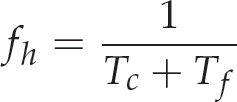
where

v_{1} = \frac{d}{dt} z_{Δ} (T_{c}) = v_{0} e^{- \frac{c π}{2 M_{L} ω_{d}}}

(10)

Accordingly, the total hopping frequency is defined as:

f_{h} = \frac{1}{T_{c} + T_{f}}

(11)

Finally, the energy loss caused by the damping factor c_s can be obtained from the difference of kinetic energies:

Δ E_{K} = E_{K} |_{v_{1}} - E_{K} |_{v_{0}} = \frac{M_{L} v_{0}^{2}}{2} (e^{\frac{- c_{s} π}{M_{L} ω_{d}}} - 1)

(12)

As mentioned, the difference in kinetic energy can be measured indirectly as the difference in the potential energy at the apex of the two consecutive hops:

Δ E_{K} = Δ E_{P}

(13)

The damping factor c_s can be obtained from (12) as:

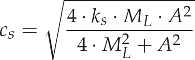
c_{s} = \sqrt{\frac{4 \cdot k_{s} \cdot M_{L} \cdot A^{2}}{4 \cdot M_{L}^{2} + A^{2}}}

(14)

where

A = - \frac{M_{L}}{π} \ln (\frac{2 \cdot Δ E_{P}}{M_{L} \cdot v_{0}^{2}} + 1)

(15)

In order to evaluate the presented foot design two experimental platforms were used. The experimental platform called Planarizer, depicted in Figure 11, uses a rotational boom to suspend the motion of the single leg. This platform is widely used for the experiments with legged robot platforms [3, 17]. The planarizer constrains the motion of the leg to 2D space (i.e. horizontal and vertical motion) and ensures that the leg follows a circular path, which in turn allows for the leg to cover long distances and prolongs the experiments. The leg behaviour during motion is tracked with the Smartek GigE camera [35] providing the motion tracking frequency of up to 75Hz. The setup for motion tracking is made out of one infrared marker (see Figure 11) placed on the leg. This marker is tracked and its position is analysed for identification and control purposes.

Figure 11.

Planarizer - the experimental platform with a rotational boom

The second experimental platform is the quadruped robot Dynarobin already depicted in Figure 2.

In order to calculate damping (14) the following values from Figure 10 are necessary: the initial height h₀, the initial contact speed υ₀, the final height h₁ and the mass M_L. The hip and knee joints are fixed (extended leg position) and the leg with mass M_l = 0.7kg (leg + planarizer bar) is repeatedly released from different heights h₀. One example of the tracked marker starting at height h₀ = 0.262m is depicted in Figure 12. The height difference value Δh is used to calculate the potential energy losses (13). In total, the leg was released from nine different heights h₀ and also for nine different angles α = 0°, 22.5°, 45°, 67.5°, 90°, 112.5°, 135°, 157.5° and 180°, yielding the total of 81 tests. The blue circles of which some are ovelapping represent the results of all tests for the damping c_s (see Figure 13). Finally, the third-order approximation of c_s with respect to a marked red in Figure 13 is represented analytically as:

Figure 12.

The example of tracked IR marker position

Figure 13.

Spiral foot damping c_s as a function of angle α[°]

c_{s} (α) = 5.11 \cdot 10^{- 6} \cdot α^{3} - 0.001 \cdot α^{2} + 0.0826 \cdot α + 0.8123

(16)

The final values for the characteristic angles are listed in Table 4. The approximation of energy losses is also calculated based on obtained Δh values and goes from 19.5% (α = 0°) towards 73.6% at α = 180°.

Table 4.

Spiral foot damping depending on the angle α

α[°]	c_s [Ns / m]	ΔE [%]	α[°]	c_s [Ns / m]	ΔE [%]
0.0	0.81	19.5	112.5	4.55	55.2
22.5	2.21	29.5	135.0	6.07	57.8
45.0	2.94	46.7	157.5	8.66	60.1
67.5	3.33	50.1	180.0	12.67	73.6
90.0	3.76	52.2

The previous stiffness and damping identification experiments have shown that the presented foot design is able to change stiffness from the minimal k_s = 1253 N / m at α = 0° to the maximal k_s = 8600 N / m at α = 180° and recover the energy from the previous hop which goes up to 80% at the minimum contact angle value α = 0°. As pointed in introduction, the possibility to adjust the leg stiffness to the desired locomotion stride frequency and the ability to partially recover the energy from the previous hop confirms the contribution of spiral foot design in lowering the total energy cost of locomotion.

3.1 Contact angle adaptation

Foot deflection during the stance phase is measured by a flex sensor and transformed into a suitable digital value denoted as AD value by using the microcontroller dsPIC30F4013. The result of deflection measurement can be used for determination of T_flex, the time elapsed from the initial contact (start of the stance phase) to the foot maximum deflection (see Figure 10).

In order to analyse the leg behaviour on different surfaces a simple control design is introduced as shown in Figure 14. When the foot reaches maximum deflection, the microcontroller triggers the main computer to actuate the leg and to generate force on the foot in -z direction. This movement adds additional energy to the system and allows jumps of a single leg above the ground. During the flight phase the microcontroller calculates interval T_flex from the previous hop, which is then used as a feedback for the foot contact angle adaptation algorithm. The aim of a leg surface adaptation experiment is to show that the time interval T_flex can remain constant in case of hopping on different surfaces if the contact angle of the spiral foot is properly adjusted. Based on the measured time T_flex, the adaptation algorithm changes the foot angle α in order to reach a targeted reference time T_flex0.

Figure 14.

The control design

The example of the flex sensor AD values acquired during the stance phase are shown in Figure 15. The initial deflection value during the monitored flight phase is AD₀ = 2200. Any change bigger than the threshold value ΔAD_min triggers the microcontroller to start receiving flex sensor data. The blue coloured AD signal represents the feedback of the leg without actuation during the stance phase. It can be seen that the maximum deflection is reached in time T_flex = 0.04 s and the starting AD₀ value is reached again in T_SU = 0.082 s. The red coloured AD signal represents the actuated leg which generates force during the second part of the stance phase. The total stance phase is extended to T_SA = 0.1 s, which is the result of additional energy added to the system. This experiment confirms that the leg actuation force is generated right after the maximum deflection moment because the measured time T_flex for the red and blue AD values are equal.

Figure 15.

The flex measured value AD

If the leg starts to generate force significantly before or after the actual maximum deflection moment, the total energy added to the system is lessened. During experiments it was found that for contact angles higher than 60° the leg actuation with Dynamixel motors was too slow to recover energy dissipation needed to make a jump. Consequently, the lower and upper limits of the contact angle adaptation range were set to 0° and 60°, respectively.

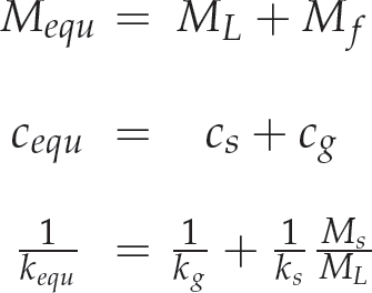
During the period of time T_flex there is no actuation and the whole leg behaves as a 2-DOF mass-spring-damper model with masses M_L and M_f, stiffness k_s, k_g and damping c_s and c_g, as shown in Figure 16. This 2-DOF model can be simplified [36] by using the 1-DOF model with mass M_equ and stiffness k_equ and c_equ defined as:

Figure 16.

2-DOF and equivalent 1-DOF spring-mass-damper system

\begin{matrix} M_{e q u} & = & M_{L} + M_{f} \\ c_{e q u} & = & c_{s} + c_{g} \\ \frac{1}{k_{e q u}} & = & \frac{1}{k_{g}} + \frac{1}{k_{s}} \frac{M_{s}}{M_{L}} \end{matrix}

The time T_flex for the 1-DOF model is defined as:

T_{f l e x} = \frac{M_{e q u} \cdot π}{\sqrt{4 k_{e q u} M_{e q u} - c_{e q u}^{2}}}

(17)

The experiments were conducted on three types of surfaces as shown in Figure 17: hard wood, single and double layer sponge with thickness of d = 0.02m and d = 0.04m, respectively. The sponges were placed on the wooden floor. The hard wood surface was very stiff in comparison to the foot and the estimated hard wood stiffness was about k_gw = 11000 N / m. The estimated damping value was negligible, c_gw = 0 Ns / m. A complex theory explains that the material stiffness and damping depend also on the contact area between two objects in collision [37]. The total surface deformation Δd in the stance phase depends on the material stiffness, contact area and initial kinetic energy of the leg at the moment of initial contact.

Figure 17.

Single leg surface adaptation: a) Hard wood surface. b) Single layer sponge. c) Double layer sponge.

In the experiments carried out the stiffness and damping of the sponge surface were determined experimentally. The foot being in contact with the single layer sponge surface at the contact angle α = 180° was much stiffer than the sponge, which ensured good estimation of the sponge parameters. During hopping on the double layer sponge the surface deformation never exceeded 75% of the total thickness d = 0.04m. In contrary, the surface deformation of the single layer sponge reached the maximum d = 0.02m and therefore, the total effective stiffness consisted of sponge and wood stiffness in series. Based on the experimental measurements the resulting single layer sponge stiffness was around k_gs = 1800 N / m. The experimentally obtained stiffness and damping coefficients for the double layer sponge surface were k_gds = 800 N / m and c_gds = 4 Ns / m.

The foot contact angle adaptation algorithm is related to stride frequency, which means that it is executed once in each hop interval of the robot leg:

α (h o p) = α (h o p - 1) + K_{γ} [T_{f l e x 0} (h o p) - T_{f l e x} (h o p)]

(18)

where K_γ represents the adaptation gain, hop denotes a current hop of the leg and T_flex is defined as:

\begin{matrix} T_{f l e x} = P (α, k_{g}, c_{g}) & = & \frac{M_{e q u} \cdot π}{\sqrt{4 k_{e q u} M_{e q u} - c_{e q u}^{2}}} \\ c_{e q u} & = & c_{s} (α) + c_{g} \\ \frac{1}{k_{e q u}} & = & \frac{1}{k_{g}} + \frac{1}{k_{s} (α)} \frac{M_{s}}{M_{L}} \end{matrix}

For c_g = 0 Nm / s, the influence of k_g on P(α) for α changing from 0° to 90° is presented in Figure 18. It can be noted that the change of k_g from 800 N / m to 11000 N / m shifted the curve P(α) for approximately 0.02s and increased the slope. Also, the variation of k_g has larger influence on T_flex as the α increases. The change of c_g for three k_g values (800 N / m, 1800 N / m, 11000 N / m) is presented in Figure 19. It can be observed that the change of c_g from 0 Nm / s to 8 Nm / s shifted the curve P(α) maximally for 0.002s, with minimal changes of slope, which allowed us to neglect the c_g value in the analysis that follows. In order to calculate the adaptation gain K_γ (see equation (18)), the function P(α, k_g, c_g = 0) is linearised as:

Figure 18.

The influence of k_g on P(α), c_g = 0 Ns / m

Figure 19.

The influence of c_g on P(α), k_g, c_g): a) k_g = 800 N / m. b) k_g = 1800 N / m. c) k_g = 11000 N / m.

K_{p} (α_{0}, k_{g}) = \frac{\partial}{\partial α} P (α, k_{g}) |_{α = α_{0}}

(19)

The K_p(α₀, k_g) values for the whole range of α₀ (0° to 90°) and k_g (800 N / m to 11000 N / m) are depicted in Figure 20.

Figure 20.

The linearized K_P (α, k_g)

Based on Figure 21, the transfer function of the contact angle adaptation loop is defined as:

Figure 21.

Contact angle (leg stiffness) adaptation scheme

\frac{T_{f l e x} (z)}{T_{f l e x 0} (z)} = \frac{1}{1 + τ (z - 1)}

(20)

where the value of

τ = \frac{1}{K_{γ} \cdot K_{p} (α, k_{g})}

(21)

defines the rate of adaptation.

Because the time interval T_flex is measured in discrete time intervals defined by non deterministic duration of each hop/jump, determinism can be established in the hopping timeframe by expressing τ as a number of hops [hop] (i.e. adaptation iterations).

As depicted with the solid red coloured curve in Figure 22, a double layer sponge (k_g = 800 N / m) had the lowest gain for each angle α₀, representing thus the worst case for adaptation. This curve is approximated by the following second order function:

Figure 22.

The linearized K_P (α, k_g), side view

K_{P d s} (α_{0}) = - 3.44 \cdot 10^{- 8} \cdot α_{0}^{2} + 6.36 \cdot 10^{- 6} \cdot α_{0} - 3.92 \cdot 10^{- 4}

(22)

Upon inclusion of (22) in (21), for given α₀, T_d = 1 hop and K_Pds(α₀) → K_P, a desired minimal rate of adaptation τ can be provided on all surfaces by using the following adaptation gain:

K_{γ} (α_{0}) = \frac{1}{τ \cdot K_{P d s} (α_{0})}

(23)

which guarantees stability, based on the poles of the transfer function (20), for all τ > 0.5 hop.

3.2 Single leg experiments

The tests of the described adaptation scheme were carried out through repetitive jumps of the robot leg on three different surfaces. The actuated leg path repeatedly generated movement in -z direction Δz_a = 0.03m. The total equivalent mass is M_equ = 0.7kg (M_f ≈ 0). As discussed before, contact angle adaptation during the experiments was constrained to the range from α = 0° to α = 60°. The presence of this limit is also visible in the contact angle adaptation scheme depicted in Figure 21.

The experiments containing N = 250 hops were conducted on three different surfaces in the following order: hard wood surface, single layer sponge, double layer sponge and back over via single layer sponge to the initial hard wood surface. The surface changing interval was set to N=50 hops. The hopping result with the fixed contact angle α = 0 is presented in Figure 23 a). It can be observed that on the single layer sponge the initial T_flex = 0.041 s changes to T_flex = 0.051 s and then, on the double layer sponge, it reaches T_flex = 0.062 s.

Figure 23.

The leg surface adaptation: a) No adaptation. b) Adaptation with τ = 4 hop. c) Adaptation with τ = 2 hop. d) Adaptation with τ = 1.5 hop.

For the given reference time T_flex0 = 0.040 s, the adaptation algorithm results for three various adaptation rate values (τ = 4, 2 and 1.5 hop) are depicted in 23 b) to d). It can be observed that for all three values of τ the measured T_flex values ended in narrow interval around the reference value 0.040 ± 0.002 s. The experiments showed that adaptation rates smaller than τ = 2 hop produced larger overshoots and oscillations.

4. The Role of the Spiral Feet in Quadruped Locomotion

The experiments on a single leg have confirmed that presented revolute spiral feet design comprises the following properties:

R₁: Variable passive compliance based on single servo motor control

R₂: Detection of maximum deflection moment based on the feedback from the flex sensor mounted on the spiral feet

R₃: Reusing energy stored in the spiral feet from the previous hop / step

R₄: Surface adaptation capability based on the measured time T_flex and change of the foot contact angle α

In order to fully evaluate these properties on quadrupeds, it is necessary to fulfill some demands on the robot control structure. Based on our recent research [38][39], potential problems and necessary conditions on the robot control structure are presented hereafter, especially to evaluate the properties R₃ and R₄.

4.1 Requirements on quadruped robot control structure

There are four most common quadruped gaits: walk, trot, pace and bound. Gaits exhibit different characteristics in terms of speed, stability and energy efficiency [40, 41]. The walk gait keeps three legs in contact with the ground in every moment and it is considered to be optimal for range of fairly low speeds. The trot gait produces symmetric leg movements with respect to robot's diagonal in order to provide faster forward locomotion. The pace gait is similar to trot but the pairs are formed by the two legs on the same side. Finally, the bound gait allows the quadruped to reach higher locomotion speeds. In theory all types of four-legged gaits can assume the properties R₃ and R₄ except of the walking gait whose behavior of robot legs cannot be approximated by the SLIP model.

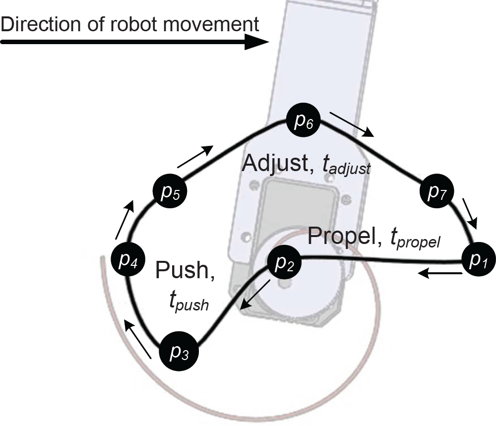
Referring to our complementary research work described in [39], the foot trajectory for all types of four-legged gaits can be described a as cyclic trajectory divided into three distinct segments (see Figure 24): the propel segment from points p₁ to p₂ where a robot is propelling itself by pushing the foot in horizontal direction while in contact with the ground; push segment lasting from p₂ and p₄ produces vertical and horizontal components of the foot take-off force; the adjust segment spanning between points p₄ and p₁ adjusts the robot leg to initial position. Each segment has respective duration time: t_propel, t_push and t_adjust. By using the proposed state machine-based approach [39], the presented foot trajectory shape can be executed on all four legs depending on a selected gait with ability to adjust positions of the trajectory points p_i and duration of the propel, push and adjust segments. The proposed approach provides ability to optimize the foot trajectory based on a multiple criterion function with arguments like speed, gait stability and energy efficiency (property R₃).

Figure 24.

Proposed trajectory shape [39]

A simplified dynamic model of a quadruped robot consists of a main body attached to four active springs each representing one robot leg. The main body can be modeled as a system of four equally displaced cuboid masses M_qi, i = 1,..,4, as shown in Figure 25. Referring to relation (17), correct measurement of T_flexi requires knowing M_qi, which is satisfied only if all gait supporting legs touch the ground at the same time. In other words, any deviation from that condition can yield inaccurate ground stiffness measurements. Deviations may occur due to many reasons such as uneven terrain configuration, imperfect robot construction, type of control, robot's task, influence of external forces etc. Some of these causes will affect the distribution of quadruped masses M_qi, other will cause that all supporting legs do not touch the ground simultaneously. In order to fulfill the goal R₄, the control algorithm must provide simultaneous actuation of all four legs (real time motor control), controllable mass distribution (tail control [38] or kinematics-based body pose adaptation [30]), active compensation of unwanted body rotations (tail control) and robust measurement of time T_flexi (initial contact and maximum deflection time), etc. In other words, the spectrum of quadruped control goals is now expanded also to possible ground stiffness adaptation.

Figure 25.

Symplified quadruped body dynamics

4.2 Preliminary experiments with quadruped robot

In order to fulfill the requirement R₃, the proposed control structure based on a three segmented trajectory can reuse the energy from the previous step if the following conditions are satisfied:

The propel phase starts when the foot touches the ground. This moment is detected by the flex sensor.

The push segment needs to start around the foot maximum deflection time. This time can be predicted by a current foot angle α.

The length of the stride period (t_propel + t_push) must be equal to the foot contact time T_c.

The transition from the adjust to the propel phase occurs at the ground contact event.

Partially reused energy from the previous step reduces the need for additional actuation energy during the push segment, which eventually reduces the total cost of locomotion. The practical confirmation of the property R₃ for robot Dynarobin is a part of future work.

In order to evaluate the requirement R₄, the quadruped hopping gait experiment with adaptation to stiffness varying surfaces is organized in a way that the robot is repeatedly released manually from the height h₀ = 0.05 m without generating any leg movement in -z direction (Δz_a = 0) during the contact phase. This ensures that all legs touches the ground at the same time. Each leg i has the ability to adapt stiffness and to measure the time T_flexi, i ∊ {1, …, 4}. In order to provide more stable results, the contact angle adaptation algorithm uses the average feedback time T_flexΣ defined as:

T_{f l e x}_{Σ} = \sum_{i = 1}^{4} \frac{T_{f l e x}_{i}}{4}

(24)

The robot is repetitively released on two different surfaces in the following order: hard wood, double layer sponge and again hard wood (see Figure 26). In total N=150 hops are conducted with a surface exchanging interval of N=50 hops. The approximated mass for each leg is M_equ = 0.75kg which includes the leg mass and the quarter of the body mass.

Figure 26.

Dynarobin experiment a) Hard wood surface. b) Double layer sponge.

Without contact angle adaptation the changes in surface stiffness result with changes of T_flex from initial 0.043 s on the hard wood to approximately 0.065 s on the double layer sponge (see Figure 27 a)). The results of adaptation algorithm can be seen in Figure 27 b). The changes in surface stiffness are successfully compensated by using the adaptation rate τ = 2hop.

Figure 27.

Quadruped surface adaptation: a) No adaptation. b) Adaptation with τ = 2 hop.

5. Conclusions

The simple mechanical design of a robot leg with an elastic spiral-shaped foot allows the leg to possess both active and variable passive compliance properties. The reuse of energy stored in the position-controlled foot spring brings such a design closer to a biological model. Efficient locomotion control requires knowing the stiffness and damping coefficients of the compliant robot leg which must be identified for different contact angles with the ground. In the article, the foot stiffness identification is performed by a strength tester TensoLab measurement system. The damping coefficient is observed through energy losses during the hopping contact phase. The analytic solution is derived using the mathematical model of a bouncing ping-pong ball. The vision tracking system is used to measure the position and velocity of the leg during hopping which is further used for calculating the damping coefficients.

The spiral foot surface adaptation algorithm is presented based on measured time T_flex obtained by flex sensor feedback. The experiments were performed on two experimental platforms, a single leg and a quadruped robot called Dynarobin. The possibility to adjust the leg stiffness and ability to partially recover the energy from the previous hop confirm the contributions of the foot design to lessening the total energy cost of locomotion. Finally, the presented experiments confirm the ability of the adaptive stiffness system to keep the changes of contact time T_c constrained in a narrow range, which is a necessary condition to obtain energy efficient quadruped locomotion. Future work will continue with solving the problem of robot stiffness adaptation to stiffness variations of natural, uneven terrains, where interference of balance control and stiffness control will be investigated.

6. Acknowledgements

This work was supported by a grant from the Ministry of Science, Education and Sports, Republic of Croatia. Special thanks to Marko Cukon, who was the Dynarobin and the spiral foot designer. Special thanks to the company MIRTA-KONTROL d.o.o. (www.mirta-kontrol.hr), the owner of the TensoLab 3000 measurement system.

References

Blickhan

. The spring-mass model for running and hopping. Journal of Biomechanics, 22(11–12):1217–1227, 1989.

McMahon

T. A.

and Cheng

G. C.

. The mechanics of running: how does stiffness couple with speed? Journal of Biomechanics, 23 Suppl 1:65–78, 1990.

Raibert

M. H.

. Legged robots that balance. Massachusetts Institute of Technology, Cambridge, MA, USA, 1986.

Blickhan

and Full

R. J.

. Similarity in multilegged locomotion: Bouncing like a monopode. Journal of Comparative Physiology A, 173:509–517, 1993.

Galloway

K. C.

. Passive Variable Compliance for Dynamic Legged Robots. dissertation, University of Pennsylvania, 2010.

Hurst

J. W.

. The Role and Implementation of Compliance in Legged Locomotion. PhD thesis, Robotics Institute, Carnegie Mellon University, Pittsburgh, PA, August 2008.

Farley

C. T.

Blickhan

Saito

, and Taylor

C. R.

. Hopping frequency in humans: a test of how springs set stride frequency in bouncing gaits. Journal of Applied Physiology, 71(6):2127–32, December 1991.

Arampatzis

Bruggemann

G. P.

, and Metzler

. The effect of speed on leg stiffness and joint kinetics in human running. Journal of Biomechanics, 32(12):1349–53, December 1999.

Farley

C. T.

Glasheen

, and McMahon

T. A.

. Running springs: speed and animal size. Journal of Experimental Biology, 185:71–86, December 1993.

10.

Full

R. J.

and Tu

M. S.

. Mechanics of a rapid running insect: two-, four- and six-legged locomotion. The Journal of Experimental Biology, 156(1):215–231, March 1991.

11.

Ker

R. F.

Bennett

M. B.

Bibby

S. R.

Kester

R. C.

, and Alexander

R. M.

. The spring in the arch of the human foot. Nature, 325:147–149, 1987.

12.

Ferris

D. P.

Louie

, and Farley

C. T.

. Running in the real world: adjusting leg stiffness for different surfaces. Proceedings of the Royal Society of London. Series B: Biological Sciences, 265(1400):989–994, June 1998.

13.

Ham

Sugar

Vanderborght

Hollander

, and Lefeber

. Compliant actuator designs. Robotics Automation Magazine, IEEE, 16(3):81–94, September 2009.

14.

Poulakakis

Smith

J. A.

, and Buehler

. Modeling and experiments of untethered quadrupedal running with a bounding gait: The scout ii robot. International Journal of Robotics Research, 24(4):239–256, 2005.

15.

Gabrielli

and von Karman

. What price speed? Mechanical Engineering, 72(10):775–781, 1950.

16.

Ahmadi

and Buehler

. Controlled passive dynamic running experiments with the arl-monopod ii. IEEE Transactions on Robotics, 22(5):974–986, October 2006.

17.

Zeglin

. The Bow Leg Hopping Robot. PhD thesis, Robotics Institute, Carnegie Mellon University, Pittsburgh, PA, October 1999.

18.

Semini

. HyQ-Design and Development of a Hydraulically Actuated Quadruped Robot. PhD thesis, Italian Institute of Technology and University of Genoa, Italy, 2010.

19.

Hutter

Gehring

Bloesch

Hoepflinger

M. A.

Remy

C. D.

, and Siegwart

. StarlETH: A compliant quadrupedal robot for fast, efficient, and versatile locomotion. In 15th International Conference on Climbing and Walking Robot - CLAWAR 2012, 2012.

20.

Raibert

M. H.

Brown

H. B.

Hastings

Koechling

Murphy

K. N.

Murthy

S. S.

, and Stentz

Anthony J.

. Dynamically stable legged locomotion. Technical report, MIT Artificial Intelligence Laboratory, 1989.

21.

Hurst

J. W.

Chestnutt

, and Rizzi

. An actuator with mechanically adjustable series compliance. Technical Report CMU-RI-TR-04–24, Robotics Institute, Pittsburgh, PA, April 2004.

22.

Wolf

and Hirzinger

. A new variable stiffness design: Matching requirements of the next robot generation. In 2008 IEEE International Conference on Robotics and Automation (ICRA), Pasadena, California, USA, pages 1741–1746. IEEE, 2008.

23.

Shin

Sardellitti

Park

Y. L.

Khatib

, and Cutkosky

M. R.

. Design and control of a bio-inspired human-friendly robot. International Journal of Robotics Research, 29(5):571–584, 2010.

24.

Saranli

Buehler

, and Koditschek

D. E.

. Rhex: A simple and highly mobile hexapod robot. International Journal of Robotics Research, 20:616–631, 2001.

25.

Johnson

A. M.

and Koditschek

D. E.

. Toward a vocabulary of legged leaping. In 2013 IEEE International Conference on Robotics and Automation (ICRA), pages 2553–2560, May 2013.

26.

Zhang

, and Goldman

D. I.

. A Terradynamics of Legged Locomotion on Granular Media. Science, 339(6126):1408–1412, March 2013.

27.

Galloway

K. C.

Clark

J. E.

, and Koditschek

D. E.

. Design of a multi-directional variable stiffness leg for dynamic running. ASME Conference Proceedings, 2007(43041):73–80, 2007.

28.

Galloway

K. C.

Clark

J. E.

Yim

, and Koditschek

D. E.

. Experimental investigations into the role of passive variable compliant legs for dynamic robotic locomotion. In 2011 IEEE International Conference on Robotics and Automation (ICRA), pages 1243–1249, May 2011.

29.

Ferris

D. P.

Louie

, and Farley

C. T.

. Runners adjust leg stiffness for their first step on a new running surface. Journal of Biomechanics, 32(8):787–94, 1999.

30.

Mutka

Petric

Reichenbach

, and Kovacic

. Elliptical motion method for robust quadrupedal locomotion. In IEEE International Conference on Control Applications (CCA), pages 1032–1038, 2012.

31.

Schmidt

and Fischer

M. S.

. Morphological integration in mammalian limb proportions: Dissociation between function and development. Evolution, 63(3):749–766, 2009.

32.

Shih

. Introduction to Finite Element Analysis Using SolidWorks Simulation 2010. Schroff Development Corporation, 2010.

33.

Italy Mesdan S.p.A. Tensolab 3000 strength tester. http://www.mesdan.com/english/scheda_lab.php/linea/2/destinazione/26/applicazione/58/prodotto/13 Accessed on 10 Mar 2014.

34.

Nagurka

and Huang

. A mass-spring-damper model of a bouncing ball. International Journal of Engineering Education, 22(2):393–401, 2006–03–01T00:00:00.

35.

Smartek cameras. www.smartek.hr/ Accessed on 10 Mar 2014.

36.

Suciu

C. V.

. Ride-comfort of an automobile equipped with colloidal dampers at its frontal suspensions. In Proceedings of ISMA2010, Belgium, pages 4233–4245, 2010.

37.

Roncevic

. Analysis of a receding contact problem. PhD thesis, University of Rijeka, July 2012.

38.

Mutka

Orsag

, and Kovacic

. Stabilizing a quadruped robot locomotion using a two degree of freedom tail. In Proceedings of 21st Mediterranean Conference on Control and Automation, pages 1336–1342, 2013.

39.

Koco

Mutka

, and Kovacic

. New parameterized foot trajectory shape for multi-gait quadruped locomotion with state machine-based approach for executing gait transitions. In Proceedings of 22st Mediterranean Conference on Control and Automation, Palermo, Italy, accepted for publication, 2014.

40.

Kar

D. C.

Issac

K. K.

, and Jayarajan

. Gaits and energetics in terrestrial legged locomotion. Mechanism and Machine Theory, 38(4):355–366, 2003.

41.

Hoyt

D. F.

and Taylor

C. R.

. Gait and the energetics of locomotion in horses. Nature, 292(5820):239–240, July 1981.

Adaptive Control of Quadruped Locomotion Through Variable Compliance of Revolute Spiral Feet

Abstract

Keywords

1. Introduction

1.2 Compliance in robot leg design

4.1 Requirements on quadruped robot control structure

6. Acknowledgements

References