Sage Journals: Discover world-class research

Abstract

In this paper, we address a new method for the collision-free motion planning of a mobile robot in dynamic environments. The motion planner is based on the concept of a conventional collision map (CCM), represented on the L(travel length)-T(time) plane. We extend the CCM with dynamic information about obstacles, such as linear acceleration and angular velocity, providing useful information for estimating variation in the collision map. We first analyse the effect of the dynamic motion of an obstacle in the collision region. We then define the measure of collision dispersion (MOCD). The dynamic collision map (DCM) is generated by drawing the MOCD on the CCM. To evaluate a collision-free motion planner using the DCM, we extend the DCM with MOCD, then draw the unreachable region and deadlocked regions. Finally, we construct a collision-free motion planner using the information from the extended DCM.

Keywords

Motion Planner Collision Avoidance Collision Map

1. Introduction

The motion planning for the autonomous navigation of indoor-wheeled mobile robots has been a centre of attention for the scientific community over the last decade. Motion planning has applications in fields such as office cleaning, guiding visually impaired or geriatric patients [1] and fire detection. Researchers have developed various methods by which robots can complete their tasks without colliding with obstacles. In particular, methods using the potential field, dynamic window, velocity obstacle, vector field histogram, vector polar histogram, probabilistic roadmap and collision map have given diverse and useful results in known and unknown environments [2,3].

The potential field method and its extension for use in dynamic environments have been studied extensively in recent decades. The basic idea of this method is to fill the robot's workspace with an artificial potential field in which the robot is attracted to its target position and is repulsed by obstacles. This method is particularly attractive because of its mathematical simplicity. However, the potential field method has inherent shortcomings in its design, such as being stuck in local minima and the robot's oscillation in narrow passages [4–5]. Another area of motion planning, probabilistic roadmap (PRM) motion planning method, creates a graph of randomly generated collision-free configurations, which are then connected using a simple and fast local planning method. Actual global planning is carried out on this graph [6]. To minimize the time wasted constructing the unused portion of the roadmap, researchers proposed variant PRMs such as the Lazy PRM, Fuzzy PRM and Customizable PRM, which postpone some roadmap construction operations until the query time [7 –11].

The VFH [12 –15] algorithm with sonar sensors and the VPH [16–17] algorithm with laser scanners have been studied to obtain feasible bearing angles for obstacle avoidance and for reaching the target point.

Collision map-based motion planners consider only the collision time without tackling how to avoid collisions. Therefore, CCM-based motion planning is suitable for painting robots or rail-guided robots, which are forced to follow a given track. The CCM is a plane consisting of the travel length and the possible collision time. The CCM concept is clear and has been applied in many papers. [18 –22] However, a motion planner using only the CCM deals with the linear velocity of one or more obstacles without considering the obstacle's angular velocity.

Among these methods, we focus on CCM-based motion planning. We expand the concept of CCM to the consideration of dynamic terms. To use CCM in dynamic environments, we denote the direction of motion of the collision region as a vector in the collision map. We term the measure of collision dispersion (MOCD) as the magnitude of the vector, i.e., the predicted movement of the collision region in the L-T plane. We term the newly constructed map a dynamic collision map (DCM).

The singularity of MOCD arises when the collision angle becomes zero. To avoid this singularity, we propose a path regeneration algorithm that considers the collision angle. By using the DCM and the velocity constraints, we first generate a collision-free trajectory. We then construct a singularity-free and collision-free motion planner.

The dynamic environment is represented as a set of obstacles that have a state (x_o y_o, θ_o, v_o, ω_o). In addition, the concept of motion planning is represented as: “when given the initial state (x_s, y_s, θ_s, v_s, ω_s) and the final state (x_e, y_e, θ_e, v_e, ω_e) of a robot, plan the trajectory of v and ω required to reach the final state from the initial state as fast as possible.” The basic assumptions are as follows.

The mobile robot is treated as a circle or sphere to simplify the problem; a sphere model is rotationally invariant and is completely defined by its radius and the coordinates of its centre; thus, the complexity of the detection of collisions can be reduced.

If the radius of the obstacle is R₁ and the radius of the robot is R₂, then we replace the radius of the obstacle R₁ with R₁+R₂ and the radius of the robot R₂ with zero, i.e., the robot with radius R1 is replaced with a point robot.

The mobile robot has linear and angular velocity constraints, with the inequality functions as follows.

v_{\min} \leq v (t) \leq v_{\max}, ​ ​ ω_{\min} \leq ω (t) \leq ω_{\max}

(1)

The mobile robot and obstacles move in a flat plane.

The remainder of this paper is organized as follows. In section 2, we review the concept of the CCM. In section 3, we derive the equations of variables related to the CCM. We then define the MOCD and DCM-based on the effect of dynamic obstacles on the collision map. In section 4, we design the motion planner and describe the generation procedure for obtaining a continuous and smooth trajectory. In section 5, we present the simulated results. Finally, we give our concluding remarks in section 6.

2. Review of conventional collision map

Let us consider the case where a robot moves along the path from P_s to P_e, and the centre of an obstacle with status (x_o,y_o,θ_o,v_o,ω_o) moving along its path contacts collision point P_c after time t_c, as shown in Figure 1.

Figure 1.

Variables defined in a collision map

Table 1 shows the related symbols needed to derive the CCM and DCM.

Table 1.

Symbols used for derivation of CCM and DCM

Symbol	Meaning
P_s, P_e	Start/Stop point
θ _ci , θ _ti	Collision angle and tangential angle of i^th obstacle
x_i, y_i, θ_i, v_i, ω _i	Obstacle position, angle, linear velocity and angular velocity
x_c, y_c, l_c, t_c	Collision point, length and time
e_θ, e_l, e_s	Ellipse rotational angle, main axis and minor axis
D_l, D_t	Dispersion length on the L axis and T axis

If the moving path is larger than the obstacle size and the path is smooth in the neighbourhood of collision point Pc, then the path near collision point Pc can be approximated as a tangential line. Let us define the collision angle θ_c as the difference between the obstacle directional angle θ_o and the tangential angle θ_t of the robot path at the collision point, as shown in Figure 1.

Suppose that the moving obstacle is a circle and the moving path of a robot in the neighbourhood of the collision point is a tangential line. Let the length from P_s to the crossing point P_c be l_c and let the obstacle with velocity v_o escape the entire tangential line crossing P_c.

Next, we will show that the crossing points of the robot with the obstacle path become an ellipse in the L-T plane with centre (l_c, t_c), where the L-T plane consists of the robot's travel path and time. We assume that all positions and orientation angles are represented by the coordinates of the moving robot. Then, consider that the moving path is given by a function, y=f(x). To determine l_c and t_c, the collision point (x_c, y_c) in the X–Y plane is given as

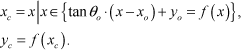
\begin{array}{l} x_{c} = x | x \in {\tan θ_{o} \cdot (x - x_{o}) + y_{o} = f (x)}, ​ \\ y_{c} = f (x_{c}) . \end{array}

(2)

From the collision point (x_c, y_c), l_c and t_c are then derived as

\begin{array}{l} l_{c} = \int_{0}^{x_{c}} \sqrt{1 + \frac{d f (x)}{d x}} \cdot d x, ​ ​ ​ ​ \\ t_{c} = \frac{D_{o}}{v_{o}}, ​ ​ ​ D_{o} \equiv \sqrt{{(x_{c} - x_{o})}^{2} + {(y_{c} - y_{o})}^{2}} . \end{array}

(3)

Let us define the following constants to obtain the rotational angle of the generated ellipse.

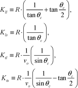
\begin{array}{l} K_{l l} \equiv R \cdot (\frac{1}{\tan θ_{c}} + \tan \frac{θ_{c}}{2}), ​ ​ ​ ​ \\ K_{l s} \equiv R \cdot (\frac{1}{\tan θ_{c}}), \\ K_{t l} \equiv R \cdot \frac{1}{v_{o}} (\frac{1}{\sin θ_{c}}), ​ ​ ​ ​ \\ ​ K_{t s} \equiv R \cdot \frac{1}{v_{o}} (\frac{1}{\sin θ_{c}} - \tan \frac{θ_{c}}{2}) \end{array}

(4)

Then, the rotational angle can be given by

e_{θ} = \frac{1}{2} \arctan (\frac{- 2}{\frac{K_{t s}}{K_{l l}} - \frac{K_{l s}}{K_{t l}}})

(5)

We subsequently define the following constants to determine the principal axis and rotational angle:

α \equiv \frac{1}{R^{2}} \cdot (1 + \frac{K_{l l}}{K_{t s}} \cdot \frac{K_{l s}}{K_{t l}}) ​

(6)

β \equiv \frac{\sin 2 e_{θ} + 2 {(\cos e_{θ})}^{2} \frac{K_{l l}}{K_{t s}}}{\sin 2 e_{θ} - 2 {(\sin e_{θ})}^{2} \frac{K_{l l}}{K_{t s}}}

(7)

e_{l} = \sqrt{\frac{β + 1}{α β}}, e_{s} = \sqrt{β} \cdot e_{l}

(8)

Among e_l and e_s, the larger value becomes the length of the main axis; the smaller value becomes the length of the minor axis in the principle axis domain.

Figures 2 and 3 show the collision region in the X–Y and L–T planes, respectively.

Figure 2.

Collision region in X–Y plane

Figure 3.

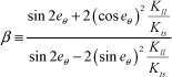
Collision region in L–T plane

Until now, researchers [2 –5] have approximated a collision region as a collision box. They have not considered the exact shape of the collision region. However, this approximation method is not practical in two aspects, the first of which is as follows. Note that the shape of the collision region is determined by the obstacle velocity υ and collision angle θ_c. As υ decreases, the length of the collision box on the t axis increases. Similarly, as the collision angle approaches zero, the length of the collision boxes on the L and T axes concurrently increase. However, the collision region always passes the point l_c+R and l_c−R at t_c, which means that the shape of the ellipsoid becomes thin. Therefore, if we approximate a collision contour as a box, then the collision box area becomes very large when compared to the ellipsoid area. In this case, there is a possibility that the solution of υ(t) and w(t) for collision-free motion planning might not be obtained, even though it exists. The second impracticality is as follows. In the case of multiple moving obstacles, if the collision regions are in one plane, then the collision regions of multiple obstacles need to be grouped according to their locations. In this case, if we do not know the exact collision contour and its boundary, we cannot guarantee mathematically that the possibility of collisions is zero in a motion planner that uses the grouping information.

3. Definition of MOCD and dynamic collision map

The collision region in Figure 3 does not include the dynamic information of an obstacle, such as acceleration or angular velocity. We thus need to analyse its effect on a collision region based on the dynamic motion of an obstacle. Figure 4 shows the variation of L when the angular velocity is changed.

Figure 4.

Variation of L when angular velocity is changed

Figure 5.

Dynamic collision map (DCM) on L–T plane

If an angular velocity w_o of the obstacle is not zero, then the collision point changes from P_c1 to P_c2; hence the travel length increases from L to L+ΔL. If we calculate the derivative of the variation of L in time, it becomes:

\begin{array}{l} \lim_{Δ t \to 0} Δ L = \cos (\frac{π}{2} - θ_{c}) \cdot \lim_{Δ t \to 0} \tan (ω_{o} Δ t \cdot D_{o}) \\ \lim_{Δ t \to 0} Δ L = \cos (\frac{π}{2} - θ_{c}) \cdot \lim_{Δ t \to 0} (ω_{o} Δ t \cdot D_{o}) \\ \frac{d L_{c}}{d t} = \frac{ω_{o} \cdot D_{o}}{\sin (θ_{c})} \equiv D_{l} \end{array}

(9)

We define D₁ as the dispersion length on the L axis, which means that the movement of a collision region changes along the L axis by the angular velocity w_o. Now, we consider the case in which the obstacle changes its velocity. In the L-T plane, t is the collision time. The time t is obtained by dividing the distance between the position of an obstacle and collision point P_c with the velocity as the obstacle moves with velocity v_o. Therefore, the variation of t_c according to the time is obtained as follows:

\begin{array}{l} (v_{o} + Δ v_{o}) (t_{c} + Δ t_{c}) = D_{o} \\ Δ v_{o} t_{c} + v_{o} Δ t_{c} + Δ v_{o} Δ t_{c} = 0 \\ \lim_{Δ t \to 0} \frac{Δ t_{c}}{Δ t} = \lim_{Δ t \to 0} \frac{- t_{c}}{(v_{o} + Δ v_{o})} \frac{Δ v_{o}}{Δ t} \\ \frac{d t_{c}}{d t} = \frac{- t_{c}}{v_{o}} \cdot \dot{v} \equiv D_{t} \end{array}

(10)

We denote D_t as the dispersion length on the t axis, which is the amount of movement of the collision region along the t axis, obtained by the linear acceleration dυ/dt.

D₁ and D_t denote two components of the collision region movement vector. We define the length of this vector as MOCD, such that

M O C D = \sqrt{{[\frac{D_{o}}{\sin (θ_{c})} \cdot ω_{o}]}^{2} + {(- \frac{t_{c}}{v_{o}} {\dot{v}}_{i})}^{2}}

(11)

The MOCD includes the physical implication of dispersion for the collision point and collision time. To estimate the exact collision point and collision time, minimizing the MOCD value is necessary. The MOCD is proportional to the angular velocity and linear velocity. From eq. (11), the singularity is generated if the collision angle θ_c or v_o becomes zero. We then define the dynamic collision map (DCM) as the map that consists of a collision region and a dispersion vector in one plane.

We want to set a new collision region that considers the MOCD after constructing the DCM in the L-T plane. To generate a collision-free motion planner with the DCM, the question that arises is how to use the information from the MOCD. In this paper, we define a new collision region using a set of ellipsoids, referred to as a collision ellipsoid set (CES). Figure 6 shows the concept of CES. If a CES is obtained, four straight lines can be generated which are tangential to the CES and their values are the maximum and minimum of υ(t).

Figure 6.

Regeneration of collision region considering MOCD and dynamic constraints

Deadlocked (inescapable) and unreachable areas are generated from the two crossing points of straight lines and from the four crossing points of the tangential lines of the CES, respectively. The deadlocked (inescapable) area is the region that a robot can enter but if it wants to exit, the velocity must exceed the maximum value. Therefore, if we plot the trajectory of x to the deadlocked area, then we cannot generate a feasible solution satisfying the entire range of x. The unreachable area is the region that a robot cannot enter because of the limitation of maximum or minimum velocity. For convenience of computation, we included the two regions in the CES.

4. Singularity-free motion planning

The MOCD has singularity when the collision angle becomes zero. In this section, we propose a path-generating algorithm that considers the collision angle.

Unlike the CCM method, which generates the trajectory using an offline method for a given path, we propose a real-time path planner to avoid singularity. The planner is generated by considering the dynamic variables of an obstacle.

Note that the path should be specified in advance to generate υ and w. Basic methods for path generation, which do not consider collision avoidance, have been widely studied and described. If two points and directional angles are defined, it is convenient to use a hermit curve. In this paper, we applied the third-order polynomial of the hermit curve to obtain f(x).

For two given position constraints and two direction constraints, let us assign the path satisfying the constraints as the third-order polynomial y=a0x³+a1x²+a2x¹+a3. Then, the coefficients can be obtained as follows:

[\begin{matrix} a_{0} \\ a_{1} \\ a_{2} \\ a_{3} \end{matrix}] = {[\begin{matrix} x_{s}^{3} & x_{s}^{2} & x_{s}^{1} & 1 \\ x_{e}^{3} & x_{e}^{2} & x_{e}^{1} & 1 \\ 3 x_{s}^{2} & 2 x_{s}^{1} & 1 & 0 \\ 3 x_{e}^{2} & 2 x_{e}^{1} & 1 & 0 \end{matrix}]}^{- 1} [\begin{matrix} y_{s} \\ y_{e} \\ \arctan (θ_{s}) \\ \arctan (θ_{e}) \end{matrix}]

(12)

In the above equation, the determinant of the matrix is -(x_s−x_e)⁴; therefore, the coefficients are unique except for in the case that x_s = x_e. Let the state of an obstacle be (x_o,y_o,θ_o,v_o,w_o). Then, the moving path of the obstacle is represented by a straight line, as in the following equation:

{y=tanθ}_{o} ({x-x}_{o}) {+y}_{o}

(13)

From eqs. (12) and (13), the intersection point of x between the third-order polynomial and the straight line is the solution of the collision point x_c. If the straight line in eq. (13) intersects the x-axis in the interval from 0 to x_e, functions that pass 0 and x_e have more than one intersection point with the straight line. Thus, even if we change function f(x) to any function g(x), we cannot completely eliminate the possibility of collision. As mentioned above, as the collision angle approaches zero, singularity occurs in the length of the moving vector in the collision region. Therefore, the path must be generated such that the collision angle is maintained at 90°, which is the core principle of our path planner. This approach matches human behaviour patterns for avoiding moving obstacles; a human typically takes a line perpendicular to the line of a moving obstacle to avoid a collision. If the collision angle is zero, then the collision vector infinitely increases in the MOCD. Therefore, the singularity avoidance algorithm is needed in order to prevent uncertainty in the path of moving obstacles.

The path-generating algorithm to maintain a collision angle of 90° is as follows:

Find the third-order polynomial that passes through the start and stop points. The directional angles in the start and stop points must match the angles of tangential lines at their points respectively.

Generate the first-order line from the state of the moving obstacle.

Search for the crossing point between the generated line and the third-order polynomial.

Define the angle for making the collision angle 90° at the crossing points.

Find the third-order polynomial g(x) connecting the start point and the collision point, which are both satisfied by tangential values at their points.

Find the third-order polynomials h(x) connecting the collision and stop points, which are satisfied by tangential values at their points.

Construct a new path connecting g(x) and h(x).

Figure 7.

Comparison of conventional path planning and singularity-free path planning

In conclusion, the generated paths satisfy the collision angle of 90° at the collision point, pass through the start and stop points, and match the pre-set steering angles at the start and stop points.

5. Simulation results and discussion

We compared the performance of the suggested DCM-based collisio1n avoidance algorithm with the VFH+ algorithm by using Matlab Simulink. To determine the steering angle with the VFH+ algorithm, it is first necessary to create a local map using 2D laser scanner data. Then, from the local map, we obtain an obstacle vector, a Primary Polar Histogram, a Binary Polar Histogram and a Masked Polar Histogram, in that order. [1] The steering angle is calculated based on the final Masked Polar Histogram. The desired steering angle is simply determined by the sum of the steering angle and the desired angle, and the steering angle error value is calculated by the difference between the desired angle and the current angle. In this simulation, we set the robot size to 0.5 m. As the real-time obstacle position is known, we performed simulations using the simulated 2D laser scanner data generated by the position data and robot size. For the DCM-based collision avoidance algorithm, we first draw DCM in the L-t plane, before moving the DCM to the x-t plane. If we suppose that the robot performs point-to-point navigation following a straight line, the x-t plane becomes the same as the L-t plane, i.e., the x-direction is the same as the robot direction. The DCM-based algorithm calculates the desired velocity and heading. However, if we control the robot's velocity, then the comparison to the VFH+ algorithm becomes meaningless because the VFH+ algorithm gives us only the desired heading. Thus, in the simulation test, we forcibly assigned a constant value to the robot's speed. Then, we compared the performance of the heading control of the DCM-based algorithm with the VFH+ algorithm. If the robot's velocity is constant and the value dx/dt is changed, then the heading value should change. With the heading variation, we can create a new via point. We assign this point to the desired point in the position control loop. Figure 8 shows the method used to calculate the via point using the heading variation. If there is no obstacle, the heading direction will be the same as the target point. Thus, the robot can arrive at the target point using this method.

Figure 8.

Method for setting a via point when the robot heading is varied

We used a quadcopter as a simulation model. The quadcopter has been studied by many researchers in recent decades. The quadcopter is a good research model to assume the shape of a circle. The DCM suggested in this paper is based on the collision avoidance of the two-dimensional space. However, various flight controllers divide the control structure with a height controller and a position controller on the horizontal plane. Therefore, we can apply our DCM algorithm to the quadcopter position controller without extension of the DCM to three-dimensional space.

We supposed that two robots (quadcopters) are flying on one horizontal plane. One quadcopter is considered as a moving obstacle and the other quadcopter as an autonomous mobile robot carrying out a given mission. In this simulation, we assume the moving obstacle moves along a given path and that the autonomous mobile robot performs a mission requiring point-to-point navigation. The two robots move on the same plane at a height of 4 m. One quadcopter follows a ‘figure-of-eight’ track, the other quadcopter moves along given positions. We assigned the target points by considering points that potentially collide with the ‘figure-of-eight’ track. Figure 9 shows the desired points and the path of the moving obstacle.

Figure 9.

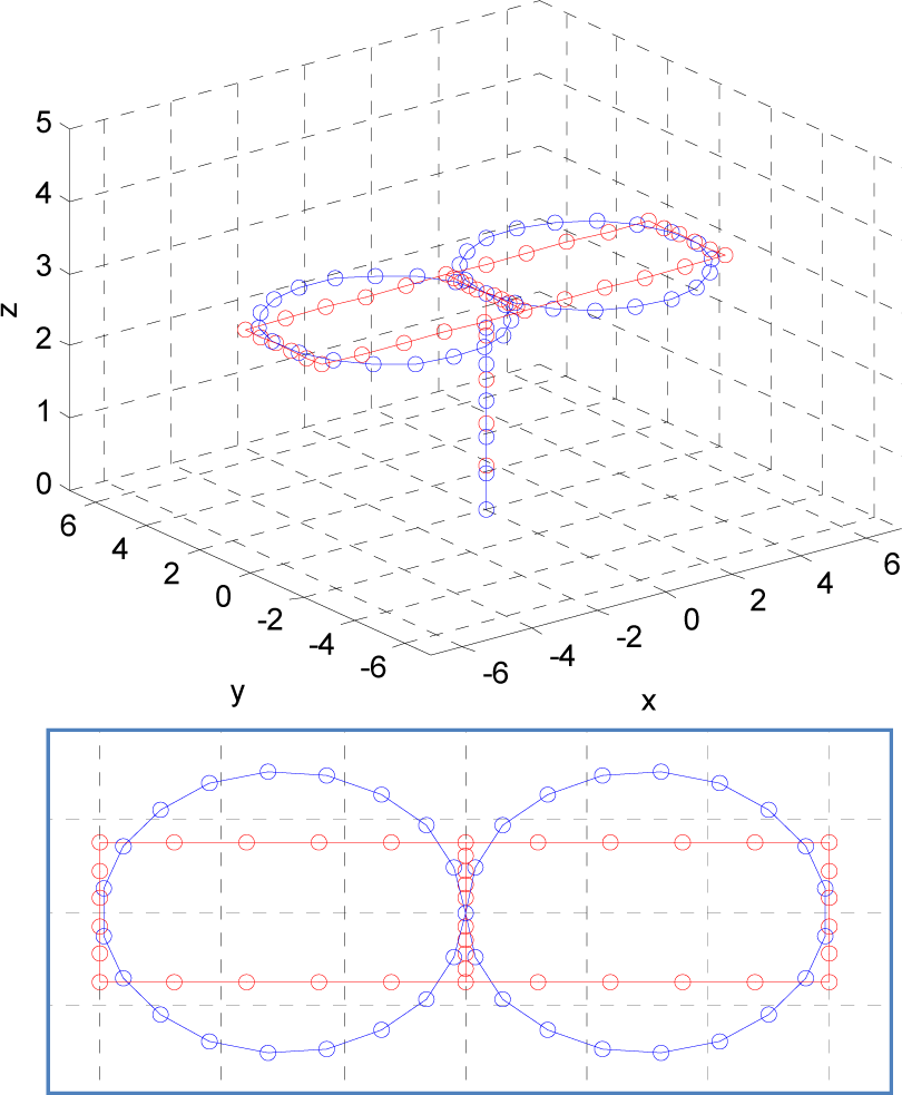
Target points of robot and moving obstacle for performing a mission

We assumed that the autonomous mobile robot can acquire the obstacle's status, e.g., position, heading value, and robot size in real time. This assumption has been a traditionally significant barrier for realizing a practical motion planner. However, the market for small-sized communication equipment, such as Zigbee and Bluetooth, has recently shown rapid growth. Therefore, this assumption has become reasonable.

We designed the quadcopter dynamic model and PID controller using Matlab 2011b Simulink. Figure 10 shows the Simulink block diagram for the suggested simulation.

Figure 10.

Block diagram of the motion planner proposed in this paper

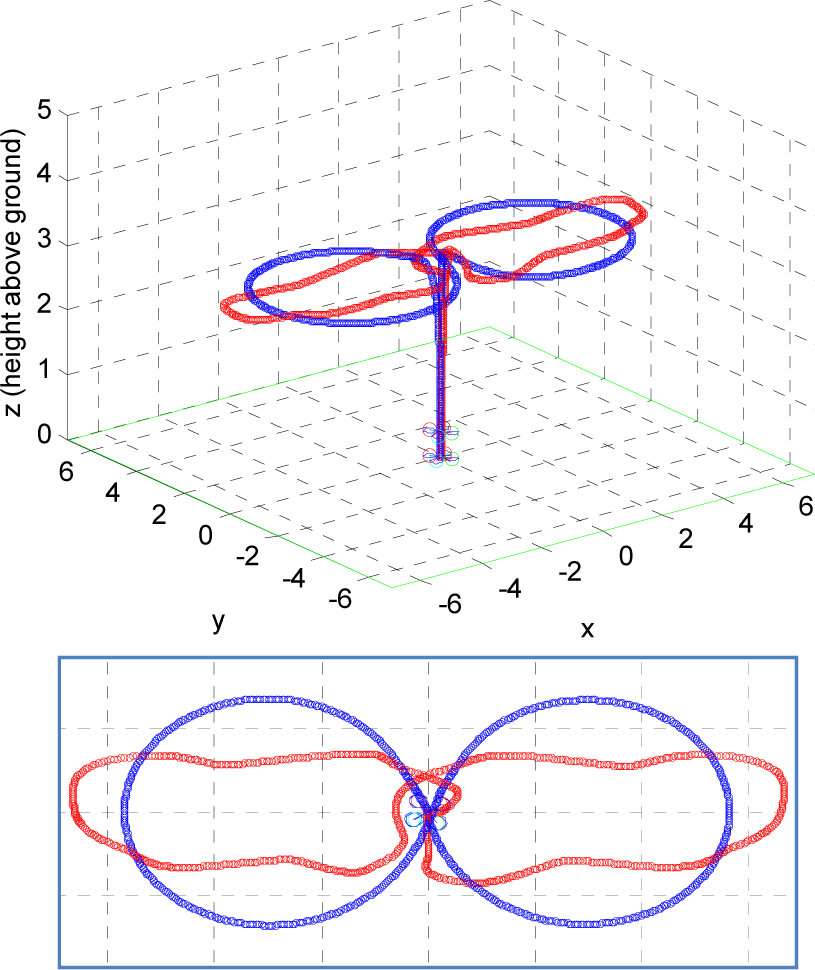
The motion planner regenerates the robot trajectory based on the input of obstacles status, robot status and waypoints at every sampling time. The output of the motion planner is the desired position, height and heading for tracking. We then compare the simulation of the VFH+ algorithm with the DCM. Figure 11 shows the tracking points of a moving obstacle and mission-performing robot when the collision avoidance algorithm is not applied.

Figure 11.

Tracks when no collision avoidance algorithm is applied

Figures 12 and 13 show the tracking points of the moving obstacle and mission-performing robot using the VFH+ and DCM-based algorithm, respectively. The definite difference of the two algorithms is whether they use the obstacle's velocity or not. The desired heading in simulation of Figure 12 was calculated by using the obstacle and target positions without considering the obstacle velocity. In contrast, the desired heading in simulation of Figure 13 was calculated by considering obstacle's velocity. After desired heading is fixed, the desired via point is calculated as shown in Figure 8.

Figure 12.

Tracks when VFH+-based collision avoidance algorithm is applied

Figure 13.

Tracks when DCM-based collision avoidance algorithm is applied

We can see the difference of shape in two tracks. The measure of performance is how well the robot follows a given track; the best algorithm minimizes the breakaway from the track. We find that the performance of collision avoidance is excellent in the two algorithms. However, the measure of breakaway is somewhat different, as the DCM-based algorithm displays less breakaway from the track.

In fact, the DCM algorithm is also more powerful in terms of velocity control. The VFH+ algorithm gives the best results for searching for the heading in a static environment. However, the algorithm does not have a similar estimation power when the obstacles are moving with changes in linear or angular velocity. In contrast, the motion planner with the DCM-based algorithm gives both the desired heading and velocity. Furthermore, the algorithm provides improved estimated results when obstacles are moving. These improvements allow the robot to change the velocity and the angle at the same time to avoid collision. As such, we can conclude that the DCM-based algorithm is more powerful than the VFH+ algorithm. However, further study is required to expand this simulation into 3D space, and to expand the simulation to include full autonomous control of velocity and heading.

6. Conclusions

In this paper, we presented a new method for collision-free motion planning of a mobile robot in dynamic environments. The main contribution of this paper is to propose a new concept for a dynamic collision map, which extends the concept of the CCM using the dynamic information of a moving obstacle. We then analysed the effect of this dynamic motion on the collision region. From this extension, we newly defined the MOCD and the DCM. We first generated a singularity-free motion planner, and subsequently verified the performance of the suggested DCM-based motion planner using Matlab Simulink simulations.

The method for grouping CESs to escape a deadlocked area will be the focus of future research, in addition to experimental tests for the suggested motion planner.

Footnotes

7. Acknowledgments

This research work was supported by the Echo Innovation Project under the Development of a Real-Time Landfill Process and Volume Measurement Technology programmes from the Korea Environmental Industry & Technology Institute (KEITI).

References

Keum-Bae

, and Beom-Hee

, “Intelligent Lead: A Novel HRI Sensor for Guide Robots”, Sensors 12, no. 6, pp. 8301–8318, 2012.

Seung

P. Hwan

, and Hee

L. Beom

, “Analysis of Robot Collision Characteristics Using the Concept of the Collision Map”, Robotica, vol. 24, pp. 295–303, May 2006.

Seung-Hwan

Heon-Cheol

, and Beom-Hee

, “Visually-Extended Vector Polar Histogram Applied to Robot Route Navigation”, International Journal of Control, Automation, and Systems, vol. 9, no. 4, pp. 726–736, Aug. 2011.

Khatib

, “Real-time Obstacle Avoidance for Manipulators and Mobile Robots”, IEEE International Conference on Robotics and Automation, pp. 500–505, St. Louis, Missouri, 1985.

Fiorini

, and Shiller

, “Motion Planning in Dynamic Environments Using Velocity Obstacles”, International Journal of Robot Res 17, no. 7, pp. 760–772, 1999.

Barraquand

Kavraki

L. E.

Latombe

J. C.

T-Y.

Motwani

, and Raghavan

, “A Random Sampling Scheme for Robot Path Planning”, International Journal of Robotics Research, vol. 16, no. 6, pp. 759–774, 1997.

Kavraki

L.E.

Kolountzakis

M. N.

, and Latombe

J. C.

, “Analysis of Probabilistic Roadmaps for Path Planning”, IEEE Transactions on Robotics and Automation, vol. 14, no. 1, pp. 166–171, 1998.

Kavraki

L. E.

Latombe

J. C.

Motwani

, and Raghavan

, “Randomized Query Processing in Robot Path Planning”, Journal of Computer and System Sciences, vol. 57, no. 1, pp. 50–60, August 1998.

Ladd

A. M.

, and Kavraki

L. E.

, “Measure Theoretic Analysis of Probabilistic Path Planning”, IEEE Transactions on Robotics and Automation, vol. 20, no. 2, pp. 229–242, April 2004.

10.

LaValle

S. M.

, and Kuffner

J. J.

“Rapidly-Exploring Random Trees: Progress and prospects”, in Donald

B. R.

Lynch

K. M.

, and Rus

(ed.), Algorithmic and Computational Robotics: New Directions, pp. 293–308. A K Peters, Wellesley, MA, 2001.

11.

LaValle

S. M.

, and Kuffner

J. J.

, “Randomized Kinodynamic Planning”, International Journal of Robotics Research, vol. 20, no. 5, pp. 378–400, May 2001.

12.

, and Wang

, “VPH: A New Laser Radar Based Obstacle Avoidance Method for Intelligent Mobile Robots”, IEEE Int. Conf. on Intelligent Control and Automation, vol. 5, pp. 4681–4685, June 2004.

13.

Borenstein

, and Koren

, “The Vector Field Histogram - Fast Obstacle Avoidance for Mobile Robots”, IEEE Journal of Robotics and Automation, vol. 7, no. 3, pp. 278–288, June 1991.

14.

Ulrich

, and Borenstein

, “VFH+: Reliable Obstacle Avoidance for Fast Mobile Robots”, IEEE International Conference on Robotics and Automation, pp. 1572–1577, May 1998.

15.

Ulrich

, and Borenstein

, “VFH*: Local Obstacle Avoidance with Look-Ahead Verification”, IEEE International Conference on Robotics and Automation, pp. 2505–2511, 2000.

16.

Gong

Duan

Man

Xiong

, “VPH+: An Enhanced Vector Polar Histogram Method for Mobile Robot Obstacle Avoidance”, Proceedings of the 2007 IEEE International Conference on Mechatronics and Automation, 2007.

17.

Dongqing

Dunlap

, and Collins

E. G.

, “A Comparison Between a Fuzzy Behavioral Algorithm and a Vector Polar Histogram Algorithm for Mobile Robot Navigating”, Proceedings of International Symposium on Computational Intelligence in Robotics and Automation, pp. 260–265, July 2007.

18.

Keum-Bae

, and Young-Dae

, “The Motion Planning of Robots Based on the Novel Analysis of Collision Map”, Korean Journal IWIT, vol. 7, pp.31–37, August 2007.

19.

Park

S. H.

, and Lee

B. H.

, “A New Analytical Representation to Robot Path Generation with Collision Avoidance through the Use of the Collision Map”, International Journal of Control, Automation and Systems, vol. 4, no. 1, pp. 77–86, February 2006.

20.

Lee

B. H.

, and Lee

C. S. G.

, “Collision-Free Motion Planning of Two Robots”, IEEE Transactions on Systems, Man, and Cybernetics , vol. SMC-17, no. 1, pp. 21–31, 1987.

21.

Sanghoon

Jeongsik

, and Hee

L. Beom

, “A Computational Interactive Approach to Multi-agent Motion Planning”, International Journal of Control, Automation, and Systems, vol. 5, no. 3, pp. 295–306, June 2007.

22.

Chang

Chung

M. J.

, and Lee

B. H.

, “Collision Avoidance for Two General Robot Manipulators by Minimum Delay Time”, IEEE Transactions on Systems, Man, and Cybernetics, vol. 24, no. 3, pp. 517–522, March 1994.

The Concept of Collision-Free Motion Planning Using a Dynamic Collision Map

Abstract

Keywords

1. Introduction

2. Review of conventional collision map

3. Definition of MOCD and dynamic collision map

4. Singularity-free motion planning

5. Simulation results and discussion

6. Conclusions

Footnotes

7. Acknowledgments

References