Sage Journals: Discover world-class research

Abstract

An approach using two intersecting circles is proposed as a linear approach for determining a camera's intrinsic parameters. The two intersecting coplanar circles have four intersection points in the projective plane: two real points and two circular points. In the image plane, the diagonal triangle - on which the image of the four intersection points composes a complete quadrangle - is a self-polar triangle for the projection curves of the circles. The vertex of the self-polar triangle is the null space of the degenerate conic formed by the image of the four intersection points. By solving the three vertices of the self-polar triangle using the image coordinates of the two real intersection points, the degenerate conic can be obtained. The image of the two circular points is then computed from the intersection points of the degenerate conic. Using the image of the circular points from the three images of the same planar pattern with different directions, the intrinsic parameters can be linearly determined.

Keywords

Camera Intrinsic Parameters Circular Points 3D Reconstruction Computer Vision

1. Introduction

In computer vision, camera calibration is a basic requirement in providing three-dimensional (3D) geometry information from two-dimensional (2D) images. This is an essential step in many visual tasks. Camera calibration techniques are used in a variety of scientific and technical fields. For example, intelligent transportation systems (ITSs) for video processing and analysis, video-based road traffic monitoring [1 –3]. Camera calibration is used for vehicle speed estimation [1], target classification and tracking [2], as well as recovering momentarily missed vehicles or distinguishing obscured vehicles [3].

Due to the importance of camera calibration, different approaches to it have been proposed for different scenarios. Traditional camera calibration approaches provide high precision but are difficult to calibrate, thus making them difficult to operate. To solve this problem, Z. Zhang [4] proposed a calibration method that utilizes a planar pattern in place of the traditional calibration object. This method is simple, convenient and low cost, though while it provides high precision it also needs to accurately determine the physical coordinates of the points in the model. C. Yang et al. [5] further developed the method of Z. Zhang [4] using the corresponding conic curves between a planar pattern and their image to calibrate a camera, rather than using the correspondence between points. Because a conic is more compact and more globally primitive, the calibration stability could be further improved. Thus, calibration approaches that use a curve have been studied extensively [6 –8]. A new, easy approach to camera calibration has been proposed based on circular points [9]. This approach utilizes a circle and a pencil of lines passing through the centre of it as a calibration pattern, introducing circular points into the camera calibration. Currently, circular points form the theoretical basis for camera self-calibration [10].

A circle is a special type of conic. All circles pass through circular points on a plane. One widely-studied camera calibration method uses a circle as a calibration pattern in combination with the theory of circular points [11 –28]. Y. Wu et al. [12] proposed a calibration method using parallel circles. Accordingly, the intersections of parallel circles are circular points. The calibration task can be completed by computing the intersections of the parallel circles in the images. C. Han et al. [13] discusses the positional relationship of any two coplanar circles on a plane and how they may be used to compute the intersections of conics in the image plane to obtain the image of the circular points. This method of camera calibration using circles as calibration patterns has been widely researched, and it is suitable for calibrating cameras that monitor roundabout traffic scenes. Reference [14] uses a single circle as a calibration pattern to compute a camera's intrinsic parameters. References [15 –23] use one or multiple pairs of coplanar concentric circles for calibration. References [24 –28] use two or more arbitrary coplanar non-concentric circles for camera calibration. The above-mentioned methods require multiple concentric or coplanar circle patterns. Based on the above research, we use two intersecting circles as a calibration pattern to calculate the intrinsic camera parameters. Two intersecting circles intersect at four points in a projective plane. According to this property, an image of the four points comprises a complete quadrangle in the image plane. Using the theory of epipolar geometry, the image coordinates of the two circular points can be solved for. By solving for the images of the circular points in three images of the same planar pattern from different orientations, the intrinsic parameters can be linearly determined. Our experimental results show that this approach is precise and effective.

The rest of this paper is organized as follows. Section 2 describes the pinhole camera model and the proposed camera calibration method using two intersecting linear circles. Section 3 presents the experimental results. Section 4 provides concluding remarks.

2. Notation and Basic Equations

In this section, we describe a pinhole camera model. We then describe the method for computing the image of the circular points from the two intersecting circles.

2.1 Pinhole Camera Model

Figure 1. Pinhole camera geometry. C represents the camera centre and is placed at the coordinate origin. O is the principal point. Note that the image plane is placed in front of the camera centre.

Figure 1.

Pinhole camera geometry. C represents the camera centre and is placed at the coordinate origin. O is the principal point. Note that the image plane is placed in front of the camera centre.

A 3D point is denoted by M = [X,Y,Z]^T and a 2D point in the image plane is denoted by m = [u, v]^T; their homogeneous point coordinates are denoted by M͂ = [X,Y,X,1]^T and m͂ = [u, v,1]^T. The camera is a pinhole model, as shown in Figure 1 [10]. In the pinhole camera model, a point in space with coordinates M =[X,Y,Z]^T is mapped to the point in the image plane where a line joining the point M to the centre of the projection meets the image plane. Using similar triangles, one can quickly compute that the point [X,Y,Z]^T is mapped to the point [fX/Z, fY/Z, f]^T in the image plane. Ignoring the final image coordinate, we can see that [X, Y, Z]^T → [fX/Z, fY/Z]^T describes the central projection mapping from the world to the image coordinates. If the world and image points are represented by a homogeneous vector, the central projection is expressed simply as a linear mapping between the homogeneous coordinates, as follows:

(\begin{matrix} X \\ Y \\ Z \\ 1 \end{matrix}) \mapsto (\begin{matrix} f X \\ f Y \\ Z \end{matrix}) = [\begin{matrix} f & 0 \\ f & 0 \\ 1 & 0 \end{matrix}] (\begin{matrix} X \\ Y \\ Z \\ 1 \end{matrix})

(1)

This can be written compactly as m͂ = PM͂, defining the camera matrix for the pinhole model of the central projection as P = diag(f,f,1) [I|0] . If one considers the principal point offset, equation (1) may be expressed in homogeneous coordinates as:

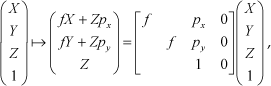
(\begin{matrix} X \\ Y \\ Z \\ 1 \end{matrix}) \mapsto (\begin{matrix} f X + Z p_{x} \\ f Y + Z p_{y} \\ Z \end{matrix}) = [\begin{matrix} f & p_{x} & 0 \\ f & p_{y} & 0 \\ 1 & 0 \end{matrix}] (\begin{matrix} X \\ Y \\ Z \\ 1 \end{matrix}),

(2)

where [p_x, p_y]^T are the coordinates of the principal point.

Because $K = [\begin{matrix} f & p_{x} \\ f & p_{y} \\ 1 \end{matrix}]$ , the matrix K is the camera calibration matrix. If one considers the camera rotation and translation, the points in space are expressed in terms of a different Euclidean coordinate frame, known as the ‘world coordinate frame’. The two coordinate frames are related through a rotation and translation. From (2), m͂ = KR[I |-C͂]M͂, where C͂ represents the coordinates of the camera centre in the world coordinate frame and R is a 3 × 3 rotation matrix representing the orientation of the camera coordinate frame. Let P = KR[I |–C͂] . It is often convenient not to make the camera centre explicit. Thus, the camera matrix is P = KR[I|t], where t = −RC͂.

This pinhole camera model assumes that the image coordinates are Euclidean coordinates with equal scales in both axial directions. In the case of CCD cameras, there is the additional possibility of having non-square pixels. Measuring the image coordinates in pixels has the effect of introducing unequal scale factors in each direction. In particular, if the numbers of pixels per unit distance in the image coordinates are m_x and m_y in the x and y directions, respectively, then the transformation from world coordinates to pixel coordinates is obtained by multiplying K on the left by diag(m_x,m_y,1) . Thus, the general form of the calibration matrix of a CCD camera is:

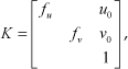
K = [\begin{matrix} f_{u} & u_{0} \\ f_{v} & v_{0} \\ 1 \end{matrix}],

(3)

where f_u = fm_x and f_v = fm_y represent the focal length of the camera in terms of pixel dimensions in the X and Y directions, respectively. Similarly, (u₀,v₀) is the principal point in terms of pixel dimensions, with the coordinates u₀ = m_x P_x and v₀ = m_y P_y . For added generality, we can consider a calibration matrix of the following form:

K = [\begin{matrix} f_{u} & s & u_{0} \\ 0 & f_{v} & v_{0} \\ 0 & 0 & 1 \end{matrix}]

(4)

The added parameter s is referred to as the skew parameter. The skew parameter is zero for most normal cameras. However, in certain unusual instances, it can have non-zero values.

The projection relationship between a space point M and its image point m is:

λ \tilde{m} = P \tilde{M} = K [R t] \tilde{M},

(5)

where λ is a non-zero scale factor, P is the camera projection matrix, (R, t) is the extrinsic rotation matrix and translation vector, and K is the camera intrinsic matrix. $K = [\begin{matrix} f_{u} & s & u_{0} \\ 0 & f_{v} & v_{0} \\ 0 & 0 & 1 \end{matrix}]$ , where the coordinates of the principal point are (u₀, v₀), f_u and f_v are the scale factors of the u and v axes in the image, respectively, and s is the skew factor.

2.2 Computing the Image of Two Circular Points

Suppose there are two intersecting circles in a plane of the world coordinate system, with two real intersection points A,B (Figure 2). Any circle that passes through the circular points I, J has two intersection circles and four intersection points in the extensional Euclidean plane, denoted by A, B, I, J, respectively.

Figure 2.

Template plane including two circles

In Figure 3, the points m_A, m_B are images of intersections A,B, m_I, m_J are the images of the circular points I, J, and C₁, C₂ are the projected curves of the two intersection circles Q₁, Q₂. These curves still intersect in the image plane. The intersection points are denoted by m_A, m_B . Conic C, which passes through the four image points m_A,m_B and m_I, m_J, can be described as a linear combination, as follows:

C = C_{1} + μ C_{2}, μ \neq 0

(6)

Figure 3.

The image of the template plane including the two circles

Figure 3. The image of the template plane including the two circles

Because any three points m_A,m_B, m_I,m_J are non-collinear, the four points form a complete quadrangle and the intersection point v_i forms a pair of lines l_i and l′_i (i = 1,2,3), as shown in Figure 3. Based on the theory of projective geometry, Δv₁v₂v₃ is the self-polar triangle of conic C [29]. Thus, the maximum of the three curves degenerates as these curves pass through the four points, thereby satisfying the following equation:

\det (C) = \det (C_{1} + μ C_{2}) = 0

(7)

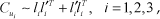
C₁, C₂ can be obtained from the image plane. In (7), the constraint is a cubic polynomial equation of μ that has three solutions, denoted by μ_i,i = 1,2,3. Thus, the three corresponding degenerate conics $C_{μ_{i}}$ can be obtained.

The three degenerate conics are of rank two. Therefore, they can be written as:

C_{u_{i}} \sim l_{i} {l^{'}}_{i}^{T} + {l^{'}}_{i} l_{i}^{T}, i = 1, 2, 3,

(8)

where l_i and l′_i are three pairs of lines in the image plane, as shown in Figure 3.

Proposition. If $C_{μ_{i}}$ is obtained according to:

l_{i} \times {l^{'}}_{i} \sim n u l l (C_{μ_{i}}),

(9)

the intersection point v of a pair of lines l_i and l′_i can be computed.

Proof. Let $C_{μ_{i}}^{*}$ be the adjoined matrix of $C_{μ_{i}}$ . From (8), we can know the following:

C_{μ_{i}}^{*} l_{i} = C_{μ_{i}}^{*} {l^{'}}_{i} = 0, i = 1, 2, 3

(10)

C_{μ_{i}}^{*} l_{i} \times C_{μ_{i}}^{*} {l^{'}}_{i} = C_{μ_{i}} (l_{i} \times l_{i}^{'}) = 0

(11)

v_{i} = l_{i} \times l_{i}^{'}

(12)

In other words, v_i is the null space of $C_{μ_{i}}$ . Solving for the three vertices of the self-polar triangle v_i from (11), with the coordinates of m_A,m_B, the images m_I,m_J of circular points can be computed from the intersection points of the lines.

2.3 Linearly Solving the Camera's Intrinsic Parameters

The circular points are on the absolute conic Ω_∞, so images m_I, m_J of the circular points are on ω = K^−TK⁻¹ [10]. The image coordinates of two circular points satisfy the following constraint equations:

m_{I}^{T} ω m_{I} = 0, m_{J}^{T} ω m_{J} = 0

(13)

Because I, J form a pair of conjugate points, under the perspective transformation, m_I, m_J also form a pair of conjugate points. Hence, the constraints of the two equations in (13) are identical.

A conic can be represented in the form of a symmetric matrix. Let:

ω = K^{- T} K^{- 1} = [\begin{matrix} c_{11} & c_{12} & c_{13} \\ c_{12} & c_{22} & c_{23} \\ c_{13} & c_{23} & c_{33} \end{matrix}] .

(14)

Define a six-dimensional vector:

c = {[c_{11}, c_{12}, c_{22}, c_{13}, c_{23}, c_{33}]}^{T} .

(15)

Let m_I = [m_I1,m_{I
2},m_{I
3}]^T . From (13):

A c = 0,

(16)

with A = [m_I1m_I1,m_I1m_{I
2} + m_I2m_I1,m_I2m_{I
2},m_I3m_I1 + m_I1m_I3,m_I3m_{I
2} +m_I2m_I3,m_I3m_I3]. Because A is a complex vector and c is a real vector, equation (16) is equivalent to the following two homogeneous equations:

[\begin{matrix} Re (A) \\ Im (A) \end{matrix}] c = 0

(17)

If n pictures of a model plane are taken in different orientations, the stack of n, as in (17), is:

V c = 0,

(18)

where V is a 2n × 6 matrix. If n ≥ 3, c can be uniquely determined up to a scale factor. The solution from (18) is well known as the eigenvector of VV^T associated with the smallest eigenvalue. Once c is obtained, we can obtain the symmetric positive definite matrix ω. Then, K⁻¹ can be computed using the Cholesky factorization [10]. The computation of the Cholesky factorization is B = LL^T, where B is a n × n symmetric positive definite matrix and L is a n × n lower triangular matrix. K can be obtained from the inverse of K⁻¹ .

Summarizing the above discussion, the camera calibration algorithm proposed in this paper is outlined as follows:

Step 1. Make a calibration pattern, as in Figure 2.

Step 2. Take three or more images of the pattern in different orientations by moving either the pattern or the camera.

Step 3. For each image, detect the feature points [30], extract the pixels u from the images of the two intersecting circles, and fit them with u^TC₁u = 0 and u^TC₂u = 0 to obtain C₁, C₂ by least squares fitting [31].

Step 4. According to (9), solve for the sides of the complete quadrangle. The image of the circular points can be obtained by computing the intersection points of corresponding sides.

Step 5. Solve for the image of the circular points in the three images of the same planar pattern in different orientations. The camera's intrinsic parameters can be linearly determined, as shown in Section 2.3.

3. Experiments

We performed a number of simulations and real experiments to verify that our approach is effective and operable.

3.1 Simulation Experiments

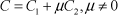
For the computer simulations, the camera settings for the intrinsic parameters were f_u = 1800, f_v = 1600, s = 10, u₀ = 800, v₀ = 600, and image resolution = 2000×1600. In the experiments, we used three images, with rotation angles and translation vectors with respect to three coordinate axes of α₁ = πl4, β₁ =π/6, γ₁ = π/8, T₁ = [300, 500, 800]^T; α₂ = π/8, β₂ =π/5, γ₂ = π/6, T₂ = [–300, 0, 400]^T; and α₃ = −π/3, β₃ = π/4, γ₃ = π/7, T₃ =[500, 650, 700]^T . 50 points were distributed uniformly on every circle. Gaussian noise with a mean of 0 and a standard deviation σ was added to the projected image points. The noise level ranged from 0 to 6.8 pixels. For each noise level, we performed 100 independent trials. The average values were calculated using a computer. Under the same conditions, several previously-used approaches [4, 9, 12] were also simulated. The absolute errors for the five intrinsic parameters under different noise levels are shown in Figure 4. We can see from Figure 4 that the calibration results are comparable and that the variances are almost linear with noise. For high noise levels, the proposed approach was robust. Thus, good camera calibration results were obtained, even with high noise levels.

Figure 4.

The absolute errors for the five intrinsic parameters (a) f_u, (b) f_v, (c) u₀, (d) v₀ and (e) s for different noise levels

Figure 4. The absolute errors for the five intrinsic parameters (a) f_u, (b) f_v, (c) u₀, (d) v₀ and (e) s for different noise levels

The second set of simulation experiments investigated performance with respect to the number of images. The settings for the first three images were the same as in the first experiment. For the fourth image, we randomly selected a rotation axis from a uniform sphere with a rotation angle of 30 degrees. We varied the number of images from 3 to 10. For each image, Gaussian noise with a mean of 0 and a standard deviation of 1 pixel was added to the projected image points. 50 trials for independent plane orientations were conducted. Several previously-used approaches [4, 9, 12] were also simulated with the same conditions. The results are shown in Figure 5. We can see that: (i) the errors decreased when more images were used, and (ii) the errors decreased significantly as the number of images increased from three to eight.

Figure 5.

Error vs. number of images: (a) f_u, (b) f_v, (c) u₀, (d) v₀

3.2 Experiments with Real Images

A series of real experiments verified our method. For the real experiments, real images were taken with a CCD digital camera. The image resolution was 640×480. We used a calibration object with two CDs, as shown in Figure 6(a). We captured three or more images of the template in different orientations by moving either the plane or the camera. We then selected three of the best images as the experimental pictures. The edges were extracted using Canny's edge detector (Figure 6(b)), and the ellipses were fitted using a least squares ellipse-fitting algorithm (Figure 6(c)) (Step 3 of our algorithm). When the equations of the two ellipses were obtained, the four intersection points were computed from the equations of the curves. For comparison, we used the approaches from references [4, 9, 12]. We took 10 images for each calibration object. Some of the sample images are shown in Figures 7(a)–9(a). The ellipses were obtained using a least squares ellipse-fitting algorithm, as shown in Figures 8(b)–9(b). The results of the five approaches are shown in Table 1. From Table 1, one can see that the calibration results obtained using these methods are similar.

Figure 6.

(a) An image of the template plane, (b) detection of the feature points, (c) curve-fitting of the ellipse

Figure 7.

(a) Image of the template planes in reference [4], (b) detection of the feature points

Figure 8.

(a) Image of the template plane from reference [9], (b) curve-fitting of the ellipse

Figure 9.

(a) Image of the template plane from reference [12], (b) curve-fitting of the ellipse

Table 1.

The results obtained using the four approaches

	f _u	f _v	s	u ₀	v ₀
Our approach	687.6959	681.8776	0.2572	303.7412	225.7260
Zhang [4]	693.5483	691.0668	-0.2377	305.2448	228.7401
Meng [9]	684.2375	691.1307	-0.8244	296.0372	206.9935
Wu [12]	688.5735	693.1190	1.0671	290.2208	211.3099

The stereo vision experiments and 3D reconstructions of the scenes were used to verify the intrinsic parameters of the camera that we proposed as a rational. If one takes two pictures using the previously-calibrated camera (Figures 10(a) and 10(b)), one will find 132 matching points from each side (indicated by the cross − 74 on the left, 58 on the right). Using the structure-from-motion method, Z. Zhang [32] was able to reconstruct the pattern using the calibrated camera's intrinsic parameters presented above. The reconstructed patterns are shown in Figure 11, in which the reconstructed points are coplanar on each side. The results demonstrate that the intrinsic parameters of the calibrated camera are accurate and precise.

Figure 10.

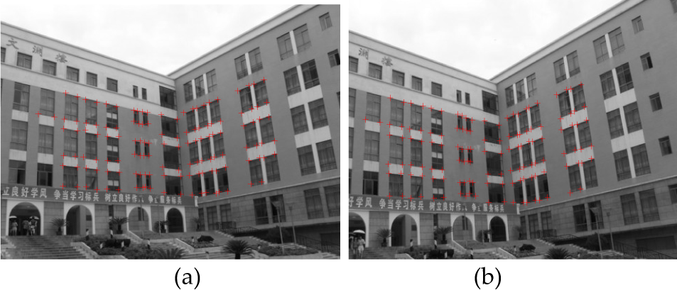
Two images (a) and (b) of the reconstruction pattern

Figure 11.

Reconstruction results

Finally, we used the intrinsic parameters shown in Table 1 to reconstruct the points in Figure 10. Using the intrinsic parameters of the four approaches, we computed the angles between two reconstructed orthogonal sections on the left and right sides (Figure 10).

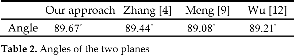
From Table 2, we can see that both are close to the ground truth of 90°. In Figure 10, we selected six row points. After obtaining the reconstructed points, we fitted the lines of the six row points using the least squares method, considered the reconstructed vertical parallel lines, computed the angles between any two of them, and obtained the averages (Table 3).

Table 2.

Angles of the two planes

	Our approach	Zhang [4]	Meng [9]	Wu [12]
Angle	89.67°	89.44°	89.08°	89.21°

Table 3.

The angles between any two of the reconstructed vertical parallel lines

	Our approach	Zhang [4]	Meng [9]	Wu [12]
Angle	0.000220°	0.000301°	0.000259°	0.000437°

Both are close to the ground truth of 0°. These results validate the proposed approach.

4. Conclusion

In this paper, we used the theory of two intersecting circles with four intersection points and an epipolar geometry in the projective plane to solve for the images of two circular points. We then linearly calculated the intrinsic parameters. This approach does not require a priori information about the circles. Instead, it only requires a camera to take three images of a template plane at a few orientations such that the intrinsic parameters can be obtained linearly. Computer simulations and real data validated our new approach. The experimental results show that this approach is precise and effective.

5. Acknowledgments

The author wishes to thank the anonymous reviewers for their many valuable suggestions. This research was supported by the Nation Natural Science Foundation of China (11361074), the Natural Foundation of Yunnan Province, China (2011FB017), and the Scientific Research Foundation of Yunnan Education Department of China (2013Y167).

References

Schoepflin

T. N.

Dailey

D. J.

, “Dynamic camera calibration of roadside traffic management cameras for vehicle speed estimation”, IEEE Trans. on Intelligent Transportation Systems, vol. 4, no. 2, pp. 90–98, Jun. 2003.

Gupte

Masoud

Martin

R. F.

Papanikolopoulos

N. P.

, “Detection and classification of vehicles”, IEEE Trans. Intelligent Transportation Systems, vol. 3, no. 1, pp. 37–47, Mar. 2002.

Pang

C. C. C.

Lam

W. W. L.

Yung

N. H. C.

, “A novel method for resolving vehicle occlusion in a monocular traffic-image sequence”, IEEE Trans. Intelligent Transportation Systems, vol. 5, no. 3, pp. 129–141, Sep. 2004.

Zhang

, “A flexible new technique for camera calibration”, IEEE Transactions on Pattern Analysis and Machine Intelligence, vol. 22, no. 11, pp. 1330–1334, 2000.

Yang

Sun

, “Planar conic based camera calibration”, Proceedings of International Conference on Pattern Recognition, vol. 1, pp. 555–558, 2000.

Tan

, “Camera calibration with conics fitting and circular points”, Journal of Xi'an Jiaotong University, vol. 40, no. 10, pp. 1065–1068, 2006.

Junejo

I. N.

Foroosh

, “GPS coordinates estimation and camera calibration from solar shadows”, Computer Vision and Image Understanding, vol. 9, pp. 991–1003, 2010.

Cao

Foroosh

, “Camera calibration and geo-location estimation from two shadow trajectories”, Computer Vision and Image Understanding, vol. 114, pp. 915–927, 2010.

Meng

Hua

, “A new easy camera calibration technique based on circular points”, in: Proceedings of the BMVC'2000, Bristol, UK, pp. 496–505, 2000.

10.

Richard

Andrew

, “Multiple view geometry in computer vision”, Cambridge: Cambridge University Press, 2000.

11.

Zhu

, “Camera calibration from the quasi-affine invariance of two parallel circles”, Proceedings of the ECCV, pp. 190–202, 2004.

12.

, “Coplanar circle, quasi-affine invariance and calibration”, Image and Vision Computing, vol. 24, pp. 319–326, 2006.

13.

Han

Liu

Dong

, “Linear approach for determining camera parameters from coplanar circles”, Computer Engineering and Applications, vol. 46, no. 1, pp. 160–163, 2010.

14.

Chen

Wada

, “Robot body guided camera calibration: calibration using an arbitrary circle”, Proc. of Inter. Conf. on Image and Graphics, pp. 39–44, 2009.

15.

Jiang

Quan

, “Detection of concentric circles for camera calibration”, Proc. of IEEE Conf. on Computer Vision, pp. 333–340, 2005.

16.

Abad

Camahort

Vivo

, “Camera calibration using two concentric circles”, Proc. of Inter. Conf. on Image Analy. and Recog., pp. 688–696, 2004.

17.

Chen

Zhao

, “A linear approach for determining camera intrinsic parameters from concentric circles”, Inter. Journal of Advancements in Computing Technology, vol. 3, no. 8, pp. 314–323, Sep. 2011.

18.

Wang

, “Calculation exact center coordinate of a target circle in camera calibration”, Infrared and Laser Engineering, vol. 40, no. 7, pp. 1342–1346, Jul. 2011.

19.

Liu

, “Nonmetric calibration of camera lens distortion using concentric circles pattern”, Proc. of Inter. Conf. on Mechanic Automation and Control Engineering, pp. 3338–3341, 2010.

20.

Zheng

Liu

, “Camera calibration using two concentric circles: linear approach”, Optical Engineering, Vol. 48, No. 5, May 2009.

21.

Wang

Yao

Cheng

, “Effective and automatic calibration using concentric circles”, Inter. Journal of Pattern Recognition and Artificial Intelligence, vol. 22, no. 7, pp. 1379–1401, Nov. 2008.

22.

Ying

Zha

, “An efficient method for the detection of projected concentric circles”, Proc. of Inter. Conf. on Image Processing, vol. 6, pp. 560–563, 2007.

23.

Kim

Gurdjos

Kweon

, “Geometric and algebraic constraints of projected concentric circles and their applications to camera calibration”, IEEE Trans. on Pattern Analysis and Machine Intelligence, vol. 27, no. 4, pp. 637–642, Apr. 2005.

24.

Chen

Wada

, “Camera calibration with two arbitrary coplanar circles”, Proc. of European Conf. on Computer Vision, pp. 521–532, May. 2004.

25.

Zheng

Liu

, “Camera calibration using one perspective view of two arbitrary coplanar circles”, Optical Engineering, Vol. 47, No. 6, Jun. 2008.

26.

Zhang

, “Self-calibration using two same circles”, Chinese Journal of Scientific Instrument, vol. 3, no. 3, pp. 618–624, Mar. 2010.

27.

Chen

, “Using coplanar circles to perform calibration-free planar scene analysis under a perspective view”, Proc. of Inter. Symp. On Advances in Visual Computing, Part I, pp. 668–677, 2009.

28.

, “Coplanar circles, quasi-affine invariance and calibration”, Image and Vision Computing, vol. 24, no. 4, pp. 319–326, Apr. 2006.

29.

Semple

Kneebone

, “Algebraic projective geometry”, Oxford University Press, 1952.

30.

Harris

Stephens

M. J.

, “A combined corner and edge detector”, Proceedings of the 4th Alvey Vision Conference, Plessey, United Kingdom, pp. 147–151, 1988.

31.

Fitzgibbon

A. W.

Pilu

Fisher

R. B.

, “Direct least-squares fitting of ellipses”, IEEE Transactions on Pattern Analysis and Machine Intelligence, vol. 26, no. 5, pp. 476–480, 1999.

32.

Zhang

, “Motion and structure from two perspective views: from essential parameters to Euclidean motion via fundamental matrix”, Journal of the Optical Society of America, vol. 14, no. 11, pp. 2938–2950, 1997.

Linear Determination of a Camera's Intrinsic Parameters Using Two Intersecting Circles

Abstract

Keywords

1. Introduction

2. Notation and Basic Equations

2.1 Pinhole Camera Model

2.2 Computing the Image of Two Circular Points

2.3 Linearly Solving the Camera's Intrinsic Parameters

3. Experiments

3.1 Simulation Experiments

3.2 Experiments with Real Images

4. Conclusion

5. Acknowledgments

References