
Abstract
In this paper we present a strategy for the problem of exploring an unknown 2D environment. Existing techniques can be methodical, goal oriented or non-reactive to additional knowledge received at each new viewpoint. We present an approach which is not goal driven, but rather seeks new unseen areas to view and explore.
The novelty of the strategy presented is the use of a view-improvement technique along with an optimal viewpoint planning method for the calculation and selection of the next-best-viewpoint. The strategy is designed for a sensor system with a limited field-of-view. Example explorations are presented and we demonstrate that the strategy finds new areas to view without exhaustive searching.
Introduction
Exploring an unknown environment is a fundamental mobile robotics problem. Many researchers concentrate on exhaustive exploration techniques such as raster scan, e.g. the Lawnmower algorithm (Arkin et al., 1993), wall-hugging (Albers et al., 1999) or circumnavigation algorithms (Kutulakos et al., 1993), (Lorigo et al., 1997); way-markers (Newman et al., 2003) and goal positions (Burgard et al., 2000) can be selected on-/off-line to aid navigation, or human path following (Althaus and Christensen, 2003) for post navigation. (Youngblood et al., 2000) use the boundaries between known and unknown parts of an environment, these frontiers are systematically selected for view as a means to expand the environment knowledge.
This paper addresses the issue of no goal position being provided and no prior knowledge of the scene. The mobile agent is to explore a completely unknown environment. The shape and size of the scene is not known, and we do not assume that all internal areas are visible or accessible. There are no way-markers to guide the agent, and once the exploration starts no human intervention is possible. Using a sensor system with a limited field-of-view, the agent must decide which direction to move and to view from its current knowledge of the scene. The only restriction placed upon the exploration algorithm is that only a limited area can be explored (to stop the agent from wandering off). If the sensor system detects features outside of this area they are ignored.
We want the agent to explore in an intelligent way, like a human might. For example, you arrive at a hotel in a city that you've never visited before. You have no map or guide to help you and therefore no knowledge of where the interesting areas are. You decide to explore the immediate area of the hotel by setting a target of exploring the area within one square mile. On leaving the hotel you take a quick scan of the hotel's surrounding buildings, and then select an area to head towards. This direction may lead to a new area to explore further, or it may lead to a dead-end.
From an initial scan of the environment at a starting position, a representation of the scene is incrementally built. To gain more knowledge of the scene, a calculation for the improvement of the view of detected obstacles allows the next move to be selected. A vision sensor system cannot differentiate between obstacles in the scene and openings which can be traversed. A confidence measure of whether world obstacles represent scene obstacles is maintained using the visibility constraint described by (Manessis and Hilton, 2005). When the view of a barrier reveals new areas (within the restricted area), these are also explored. We assume a map building algorithm that can successfully maintain information of world feature points such as those discussed in (Gartshore et al., 2002). We acknowledge that errors in this part of the system will be important for the effectiveness of the exploration and will need to be addressed for the exploration to be useful in a real system. In this paper however, we wish to draw attention to the exploration algorithm itself.
In section 2. we discuss the storage requirements for the internal representation of the world being mapped. In section 3., the calculation of hypothesised view-improvements of the world map are introduced. Section 4. reviews a next-best-viewpoint calculation to maximise the viewing angle of an opening. Example explorations of room environments are shown in section 5. The results are discussed and some conclusions drawn.
Internal Representation of the World
Vertical edge features detected in images of the scene are used to define the boundaries of obstacles. These vertical features are projected onto a 2D plan and are therefore robust to errors in detection algorithms as it is not important to detect the entire edge. Vertical edges are critical for deciding where the robot can move; detecting other features is not necessary.
Some vertical edge features such as shadows or transient objects may be added into the world map alongside real obstacle features. To allow for such artefacts to be distinguishable from real obstacles, points in the world map are labelled with a confidence measure of being real environment obstacle features; Cf is calculated from the number of sightings of the scene feature S and the number of times that the scene area is viewed V and is defined as Cf = 1 – V/S2.
Many map building algorithms store position information of scene features with no connections between the neighbouring features (Davison and Murray, 2002). Features in any world map representation alone do not provide enough information for a navigation algorithm to successfully avoid obstacles. A triangulation of the detected scene features in two dimensions generates a simple non-overlapping mesh suitable for encoding the information required for the exploration algorithm. The connecting lines between these world map features either represent real obstacles in the scene or are constructed for the triangulation (construction lines).
Construction lines are labelled with a measure of their confidence of being an obstacle using intersections of a visibility line described by (Manessis and Hilton, 2005). The constraint for a scene is such that an obstacle in the map can not intersect any line from the camera to a real obstacle. Where such a visibility line intersects a construction line this constraint is violated, therefore the construction line can not represent a real scene obstacle.
The path of the robot is deemed valid if it does not intersect any construction line labelled as an obstacle. The confidence measure of a construction line being a real obstacle Co is calculated using visibility line violations and the confidence of the features Cf to which the visibility lines are related.

The more times a construction line is intersected by visibility lines and the higher the confidence of the world feature's existence forming the visibility line, the less likely the construction line is to be an obstacle.
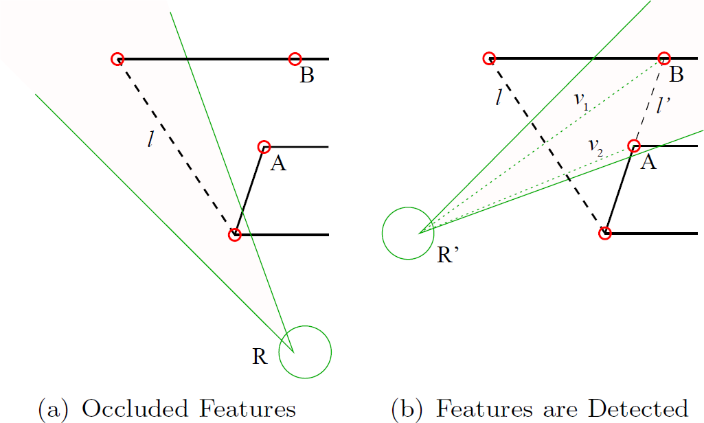
Obstacles in the world map potentially occlude unseen features in the environment. Construction lines may correctly represent real obstacles, or they may be currently labelled as such but only because thus far they have only been viewed from positions where features they occlude have not yet become visible. Figure 1(a) shows the robot at R with its camera's view direction and field-of-view. When first added into the triangulation the construction line l will be labelled as an obstacle since the features A and B have not yet been viewed. When the robot moves to position R′ (figure 1(b)), A and B are visible. The visibility lines v1 and v2 intersect the construction line l, the confidence measure Co is then recalculated.
Obstacles Viewed from Different Orientations.
When selecting a position to move to, we use the knowledge that when viewing a construction line from different positions new scene features may become visible. By storing information about the positions from which a construction line has been viewed from, we can quantify the change and therefore calculate a view-improvement for a potential viewpoint.
A 1D histogram of equal sized bins is stored with each construction line to store the angles from which the line has been viewed. Figure 2 shows such a histogram for the line l with N bins and normal vector


Obstacle Histogram Storing Angles.
The more histogram bins of a construction line that are seen and the larger the difference in the stored angles, the larger the improvement for the new view. A line viewed from the same angle but different positions does not improve the view for the line as much as viewing the line from the same position with a different view orientation.
The detection of features and their subsequent triangulation and identification of obstacles and openings greatly informs the robot exploration algorithm. However, the information that a section of the environment was viewed and that no features were detected is also useful and such information should be stored.
A simple way to store the seen parts of the world is as a discrete grid of equal sized bins forming a 2D histogram, as seen in Figure 3. For each histogram bin a[i, j] within the camera's field-of-view, the viewed angle θ can be calculated from


Area Histogram Storing Angles.
The larger the viewed and the greater the difference in the stored angles in the area's histogram, the larger the view-improvement for a new view.
Similar viewing positions provide little new information about the world map. Viewing the same features from a very similar position can improve the accuracy of the feature positions or the robot position. However, to aid the pioneering characteristic of an exploratory robot, a measure of position-similarity is used to deter a viewing position from being re-visited.
Next Viewpoint Calculation
A utility function that maximises the viewing angle of an opening is presented in (Gartshore, 2005). Figure 4 shows the robot at position r with a limited distance to move d in the presence of an opening formed by the corners C1 and C2. The point that maximises the viewing angle of the opening defines the next-best-viewpoint.
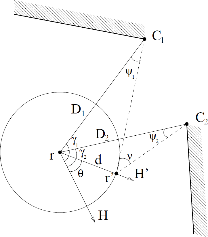
The Two Corner Case
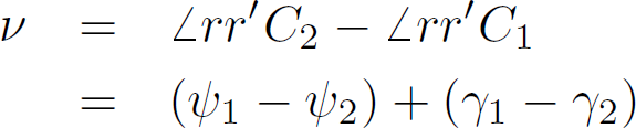
The viewing angle ν is defined by
The direction for the robot to move to reach r' is defined as θ. In the general case where D1 ≠ D2, the solution to the maximum view calculation is rearranged for θ and shown to be
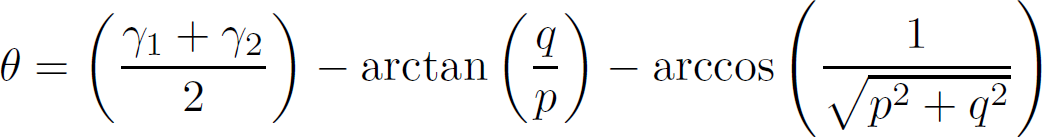

This calculation is used to find the next-best-viewpoint for a given obstacle in the world map, but is only valid when the circle defined by d remains on the same side of the opening. Since the robot path cannot intersect an obstacle, the equation will be valid.
To select which obstacle in the world map should drive the exploration, each obstacle that is visible from its next-best-viewpoint is considered. The joint-improvement for the obstacle from the next viewpoint is calculated using the position-similarity along with the addition of obstacle-view improvement and area-view improvement.
When new features are viewed and added to the map, the obstacle map expands. Newly discovered obstacles are more interesting in the exploration algorithm than obstacles that have already been viewed numerous times. When an area is found to contain new obstacles, these obstacles are prioritised. To rank new construction lines, an importance value is assigned to each obstacle and the joint-improvement for that obstacle is multiplied by this rank. The importance value is decreased each time the obstacle is used to define the next viewpoint or when the majority of the obstacle is seen, and is increased when it is first discovered during the exploration. It is increased by a value relative to the size of the new area that was discovered when the obstacle was first seen. If when the new feature is added to the map only a small new area is added, those new obstacles are not highly prioritised.
Results
Information of an unknown environment is built up over a series of moves, selected using the joint-improvement function. Move options are calculated from the set of hypothesised obstacles in the world map using the next-best-viewpoint for each obstacle. Three options of distance to move d, are used: 0mm (rotation only), 400mm and 1200mm. This allows the agent to not traverse if it has found a good position to view several obstacles from, or to quickly move to a new area if the current position does not allow for good viewpoint possibilities. If from the new viewpoint the selected obstacle is viewable by a number of orientations, options for view orientation are also calculated.
Before the exploration, no information of the position or number of obstacles in the environment is known, and the size of the environment is not estimated. The map is built relative to the starting position (0, 0). An initial scan of the environment builds up a representation of the local area. Neighbouring environment features are assumed to be obstacles until the construction line that defines the hypothesised obstacle boundary is violated by visibility constraints. As the agent moves through the scene, obstacle features detected from each viewpoint are incorporated in the world map. The confidence of each construction line being an obstacle Co is evaluated using the visibility lines from each new viewpoint.
Exploration of a Complex Map
The example environment of Figure 5 shows the initial position, almost completely surrounded by obstacles of various lengths, labelled as Area 1. After the initial scan, only 9% of the environment area will be viewed. This initial obstacle configuration is designed so that none of the sixteen external obstacles can be seen.
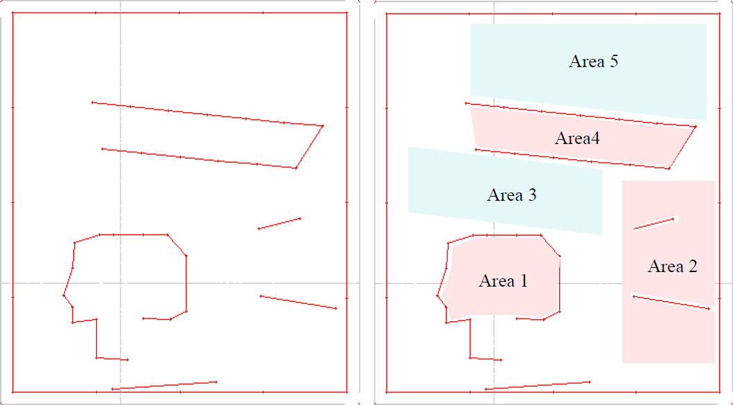
Complex Map Environment and Area Labels. Sixteen external obstacles enclose the exploration area, fifteen obstacles enclose the starting position, restricting the initial view of the environment to 9%.
The large area, Area 2, to the bottom right of the environment is occupied by two other obstacles, one very close to an external obstacle so that the agent is unable to navigate around it and also greatly restricts the view along the right-hand wall. The second smaller obstacle in Area 2 is positioned such that it can be circumnavigated by the agent, however once round this obstacle there is not much room to manoeuvre due to the exterior of the long corridor restricting the area. This scene has also been designed to highlight the long corridor and dead-end situation, Area 4.
Figure 6 shows some key snapshots of the Complex Map exploration from the starting point, within Area 1.

Complex Map Exploration: correctly detected obstacles are highlighted in red. Construction lines displayed to grey-level of Co, with Co = 1 drawn in black. Previous positions shown in green and the current position is highlighted by the field-of-view lines. Area-view histogram at move 207 (only number of entries shown) with over 95% of total area seen.
If a construction line has a very high Co value and has been at least partially seen, it is highlighted in red (the algorithm does not receive this information).
After the initial scan of fifteen rotations, only those obstacles making up Area 1 have been viewed. After 18 moves, the agent is still inside Area 1 and has not discovered that one of the obstacles is incorrectly labelled. The behaviour is such that longer obstacles are selected before shorter obstacles due to the area-and obstacle-view improvement values generally being larger because of a greater number of histogram bins for long obstacles. In confined spaces, the obstacles being selected do not tend to be those that are viewed after moving large distances. Instead the strategy of one large distance move followed by several rotations is apparent.
The agent leaves the enclosed area, after 23 moves, upon discovering new obstacles behind the previously incorrectly labelled obstacle. Each of the newly discovered obstacles are then labelled with the same value of obstacle-importance, the unanticipated new area, Area A. This large obstacle-importance value will affect each of the new obstacles such that they are more likely to be chosen by the obstacle-selection algorithm than the obstacles that make up the interior of Area A. In move 25 the rear side of an Area 1 obstacle, L4, is selected to be viewed. A purely pioneering exploration algorithm, where the only goal is to discover uncharted areas, should remove L4 from the interesting obstacle list since no new unseen area will be exposed by looking through it at any angle. The exploration presented here, however, aims to not only be pioneering i.e. search for and explore new areas, but to also enable the update of information of previously found feature positions. The ability to select this rear-side of obstacle L4 is important. In a real-world situation, obstacles will not be able to be fully represented by a single line, as all obstacles will have some depth. By allowing the rear side of obstacles to be selected for view, this will allow for the rear side of the environment obstacle to be viewed and its other points to be added to the world map accordingly.
At move 29 a new area to the bottom left of the scene, Area B, is discovered. Since the unanticipated area discovered, Area B, is relatively small compared to that from move 23, Area A, the newly added obstacles are not immediately considered for further exploration. In move 32 another large area is discovered, Area C, and the new obstacles surrounding this new area are all labelled with a very large obstacle-importance.
At move 81 an obstacle at the bottom of the scene is selected, which for the first time is viewed from an angle such that the previously occluded exterior obstacle is detected. The new area behind this obstacle is viewed further. The viewing position options of such obstacles are limited since the agent is not able to travel into the new area; the new obstacles are not immediately selected for view, but are selected once the option for a good view of the obstacle through the opening can be achieved, three moves later. The exploration continues as the path of the agent is led up and over the initial enclosing area, and the remaining unseen environment begins to be discovered. A new area to the left of Area 1 is discovered, and upon further investigation the agent travels down into the area. Up to this point, move 130, 65% of the area and 73% of the obstacles have been seen. The agent departs this confined area when an incorrectly labelled obstacle to the left of the environment is chosen for view. Rather than entering the corridor, Area 4, the obstacles selected for view are those which surround the larger new area above the corridor, Area 5. The agent travels around Area 5 for thirty moves until the position of the agent allows for the next-best-viewing position to again allow the interior of the corridor to be visible.
As the agent enters the corridor and moves towards the dead-end, the first set of moves add viewing orientations into the obstacle's histograms from only one side. As the agent proceeds down the corridor the angles added into the obstacle's histograms will be significantly different if the viewing angle is chosen to view towards the exit of the corridor. This is useful since it enables the map building algorithm to keep track of the position of the agent with respect to scene features it already knows about. After several moves inside the corridor, the agent is at the end of the corridor, at the dead-end. The area-view histogram shows that the majority of the scene area has been viewed at least once except for a few small areas to the bottom left and one to the right of the scene. At move 292 the agent has left the corridor (one hundred moves after entering it).
Figure 7 shows the distance travelled during the exploration against the value of the joint-improvement function. This distance is calculated in centimetres from the distance travelled by one of the agents wheels (assumed to be differential wheel drive). This graph enables us to re-trace the exploration with the values of the joint-improvement function at each step. The spikes in this function correspond to moves where new area or obstacles have been detected, e.g. move 23 where the value jumps from 1 × 10⁻¹ to 1 × 10¹⁴. At the start of the exploration, after some new unseen area is discovered, the value of the joint-improvement function is extremely high. This remains the case whilst new areas and obstacles are discovered. After 200 moves when the agent is inside the corridor, Area 4, the value of the joint-improvement steadily decreases towards zero. Since the distance the agent can travel in one step is small compared to the length of the corridor, several moves are spent inside the corridor. Some other measure would be required to push the agent away from the end of the corridor during consecutive moves. Once the agent exits the corridor the value returns to a normal magnitude (when compared to other exploration's joint-improvement function values once the majority of the area has been discovered).

Joint-Improvement versus total distance travelled.
Figure 8 shows the exploration of two unknown environments: a Basic Map and a Hidden Room Environment from (Gartshore and Palmer, 2005). The Basic Map shows a randomly generated map with five internal obstacles and sixteen external obstacles. 38% of the area is visible from the initial scan position. This exploration shows the agent quickly discovering the unseen area to the right of the environment. The agent proceeds across the top of the map and back viewing the remaining area to the left of the long obstacle.
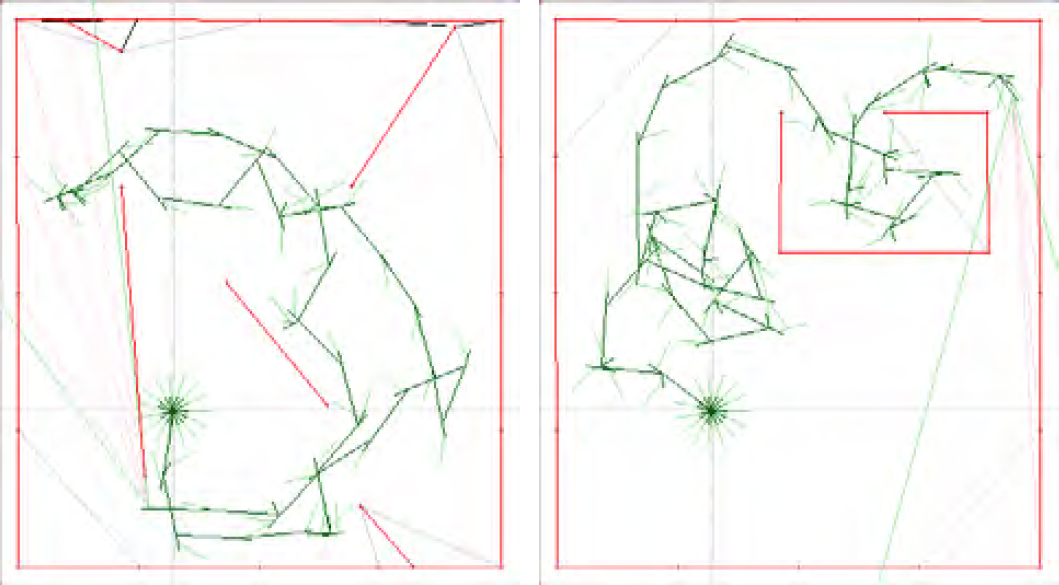
Exploration of a Basic Map and Hidden Room Environment. Obstacles are highlighted in red; all agent positions are shown in green.
In contrast to the Complex Map, where only 9% of the area is visible from the initial scan, the Hidden Room allows the majority of the area and obstacles to be seen from the starting point. This map includes a room whose entrance is hidden from the initial view location. For the agent to find the entrance to the room it must travel up to the top of the environment and look towards the entrance at an angle such that the interior of the room becomes visible. Once the room entrance is discovered and labelled as a confident opening, the agent continues its exploration moving inside. Once the obstacle- and area-view improvements decrease, the agent is pushed away from previously visited positions and exits the room. The last set of interesting obstacles is then viewed further thus completing the exploration of unknown areas in the scene.
Figure 9 shows graphs of the percentage of the area and obstacles seen against the distance travelled during the exploration of the three maps discussed. Marker 1 labelled along the graphs depicts the first move of the agent once the initial rotations are completed.

Percentage of Obstacles and Areas seen Versus Distance Travelled for explorations of three maps.
Subsequent markers then indicate the number of moves made. As we see from the sharp rise in these curves, the view-improvement exploration strategy very quickly gathers new information of the environment. For the three maps in this paper, the information gathered after the initial scan varies from 9% for the Complex Map, to 76% for the Hidden Room. The size of the map is 9m×10m. The exploration of the Basic Map is completed (i.e. all areas and obstacles viewed) within a travelling distance of 80m; 90m are travelled in the Hidden Room map to discover all the area, and 180m is travelled in the Complex Map before more than 95% of the area has been detected. As a comparison, a raster scan in this size of map without any obstacles would travel 101m (assuming a 50cm diameter agent). This Hidden Room exploration shows an improvement in excess of 20% over the raster scan approach, which is a measure of the benefit of using the view-improvement algorithm.
In this paper we have presented an exploration strategy for a sensor with a limited field-of-view. From no prior knowledge of the environment, a map representation is built up incrementally from viewing positions calculated using a next-best-viewpoint calculation. The next move is chosen from a set of options to improve upon previous views of obstacles. The exploration has been tested on a large dataset of randomly generated maps.
The novelty of this approach is the use of a set of view-improvement calculations to weight the obstacle selection for the choice of the next-best-viewpoint. We are now developing this algorithm so that it can cope with uncertainty in the map.