Sage Journals: Discover world-class research

Abstract

An efficient path planning algorithm, for multi degrees of freedom manipulator robots in dynamic environments, is presented in this paper. The proposed method is based on a local planner and a boundary following method for rapid solution finding. The local planner is replaced by the boundary following method whenever the robot gets stuck in a local minimum. This method was limited to 2-DoF mobile robots and in this work we showed how it can be applicable for a robot with n degrees of freedom in a dynamic environment. The path planning task is performed in the configuration space and we used a hyperplane in the n dimensional space to find the way out of the deadlock situation when it occurs. This method is, therefore, able to find a path, when it exists, no matter how cluttered is the environment, and it avoids deadlocking inherent to the use of the local method. Moreover, this method is fast, which makes it suitable for on-line path planning in dynamic environment. The algorithm has been implemented into a robotic CAD system for testing. Some examples are presented to demonstrate the ability of this algorithm to find a path no matter how complex is the environment. These examples involve a 5-DoF robot in a cluttered environment, then two 5-DoF robots, and finally three 5-DoF robots. In all cases, the proposed method was able to find a path to reach the goal and to avoid the dynamic obstacles.

Keywords

Path planning dynamic environment obstacle avoidance deadlock escaping boundary following

1. Introduction

Path planning is a very important issue in robotics. It has been widely studied for the last decades. The first works began in the seventies with Udupa (Udupa, S. 1977), then with Lozano-Pérez and Wesley (Lozano-Pérez, T. & Wesley, M. 1979) who proposed solving the problem using the robot's configuration space (CSpace). Since then, most of path planning important works are carried out in the CSpace. There are two kinds of path planning methods: Global methods and Local methods. Global methods (Paden, B.; Mess, A. & Fisher, M., 1989; Lengyel, J.; Reichert, M.; Donald, B. & Greenberg D., 1990; Kondo, K., 1991) act generally in two stages. The first stage, which is generally done off-line, consists of making a representation of the free configuration space (CSFree). There are many ways proposed for that: the octree, the Voronoï diagram, the grid discretization. The representation built in the first stage is used in the second one to find the path. This is not very complicated since the CSFree is known in advance. Global methods give a good result when the number of degrees of freedom (DoF) is low, but difficulties appear when the number of DoF increases. Moreover, these methods are not suitable for dynamic environments, since the CSFree must be recomputed when the environment changes. Whereas, local methods are suitable for robots with high DoF used in real time applications. The potential field method proposed by Khatib (Khatib, O., 1986) is one of the first local methods. It assumes that the robot evolves in a field of strain attracting the robot to the desired position and pushing its parts away from obstacles. Because of its local behaviour these methods do not know the whole robot's environment, and can easily fall in local minima where the robot is stuck into a position and can not evolve toward its goal. Constructing a potential field with a single minimum located in the goal position, is very hard and seems to be impossible, especially if there are many obstacles in the environment.

Faverjon and Tournassoud proposed the constraint method (Faverjon, B. & Touranssoud, P., 1987), which is a local method yielding remarkable results with high DoF robots. However this method suffers also from the local minima problem.

Probabilistic methods were introduced by Kavraki et al. (Kavraki, L.; Svestka, P.; Latombe, J-C. & Overmars M., 1996) in order to reduce the configuration free space complexity. These methods generate nodes in the CSFree and connect them by feasible paths in order to create a graph. Initial and goal positions are added to the graph, and a path is found between them. This method is not adapted for dynamic environments since a change in the environment causes the reconstruction of the whole graph. Several variants of these methods were proposed: Visibility based PRM (Siméon, T.; Laumond, J-P. & Nissoux, C., 2000), Medial axis PRM (Wilmarth, S.; Amato, N. & Stiller, P. 1999) and Lazy PRM (Bohlin, R. & Kavraki, L., 2000).

Mediavilla et al. (Mediavilla, M.; Gonzalez, J.; Fraile, J. & Peran, J., 2002) proposed a path planning method for many robots cooperating together in a dynamic environment. This method acts in two stages. The first stage chooses a motion strategy off-line among many strategies generated randomly, where a strategy is a way of moving a robot. The second stage is the on-line path planning process which makes each robot evolve toward its goal by using the strategy chosen off-line to avoid obstacles that might block its way.

Helguera et al. (Helguera, C. & Zeghloul, S., 2000) used a local method to plan paths for manipulator robots and solved the local minima problem by making a search in a graph describing the local environment using an A* algorithm until the local minima is avoided.

Simon (Simon X. Yang 2003) used a neural network method based on biology principles. The dynamic environment is represented by a neural activity landscape of a topologically organized neural network, where each neuron is characterized by a shunting equation. This method is practical in the case of a 2-DoF robot evolving in a dynamic environment. It yields the shortest path. However, the number of neurons grows up exponentially with the number of DoF of the robot, which makes this method infeasible for realistic robots.

In this paper, we propose to solve the path planning problem for many manipulator robots evolving in a dynamic environment using a real time local method. This approacch is based on the constraints method coupled with a procedure to avoide local minima by bypassing obstacles using a boundary following strategy. Section 2 describes the local method used by the planner. In section 3, the boundary following method and the projected constraints are presented. The results are shown in section 4. Finally we give some concluding remarks in section 5.

2. Local Method

In our planner, we use a local method based on an optimization under constraints process.

It is an iterative process minimizing, at each step, the difference between the current configuration of the robot and the goal configuration. When there is no obstacle in the way of the robot, we consider that it evolves toward its goal following a straight line in the CSpace. The displacement of the robot is written as follows:

\begin{aligned} Δ q_{g o a l} = \frac{q_{g o a l} - q}{∥ q_{g o a l} - q ∥} Δ q_{m a x} i f ∥ q_{g o a l} - q ∥ > Δ q_{m a x} \end{aligned}

(1)

\begin{aligned} Δ q_{g o a l} = q_{g o a l} - q i f ∥ q_{g o a l} - q ∥ ⩽ Δ q_{m a x} \end{aligned}

(2)

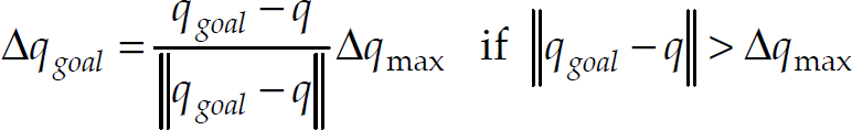
Where q_goal is the goal configuration of the robot, q is the current configuration of the robot and Δq_max is the maximal variation of each articulation of the robot. If there are obstacles in the environment, we add constraints to the motion of the robot in order to avoid collisions. Path planning becomes a minimization under constraints problem formulated as:

\begin{aligned} Minimize ∥ Δ q - Δ q_{g o a l} ∥ Under non collision constraints \end{aligned}

(3)

Where Δq is the variation of the robot joints at each step. We use non collision constraints proposed by Faverjon and Tournassoud written as follows:

\begin{aligned} \dot{d} \geq - ξ \frac{d - d_{i}}{d_{s} - d_{i}} if d \leq d_{i} \end{aligned}

(4)

With d is the minimal distance between the robot and the object, d_i is the influence distance from where the objects are considered in the optimization process, d_s is the security distance and ξ is a positive value used to adjust the convergence rate.

Fig. 1 shows two mobile objects in the same environment. The non collision constraints, taking into account the velocities of objects, are written as:

\begin{aligned} {\vec{V}}_{(x_{1} ϵ R_{1} / R_{0})} . \vec{n} - {\vec{V}}_{(x_{2} ϵ R_{2} / R_{0})} . \vec{n} \leq ξ \frac{d - d_{i}}{d_{s} - d_{i}} \end{aligned}

(5)

Fig. 1.

Two objects evolving together

Where ${\vec{V}}_{(x_{i} \in R_{i} / R_{0})}$ is the velocity vector evaluated at the point x_i of object i having the minimal distance with the second object and $\vec{n}$ is the unit vector on the line of the minimal distance.

If we consider only the velocity of the robot, and by introducing the Jacobian matrix of the robot defined in the nearest point to the obstacle, we can write the non collision constraints as:

\begin{aligned} n^{T} J_{x_{1}} (q) Δ q \leq ξ \frac{d - d_{i}}{d_{s} - d_{i}} \end{aligned}

(6)

Where $J_{x_{1}} (q)$ is the Jacobian matrix of the robot in configuration q defined in point x₁. Condition (6) will be written in the following manner:

\begin{aligned} [a_{1} \dots a_{N}] [Δ q_{1} \dots Δ q_{N}]^{T} \leq b \end{aligned}

(7)

with $[a_{1} \dots a_{N}] = n^{T} J, Δ q = {[Δ q_{1} \dots Δ q_{N}]}^{T}$ and $b = ξ \frac{d - d_{i}}{d_{s} - d_{i}}$

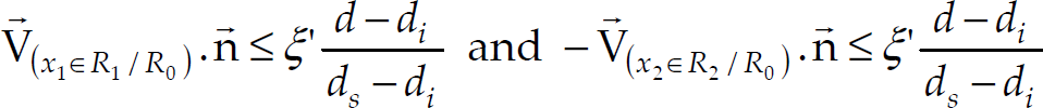
Fig. 2 shows two PUMA robots evolving together. We consider that each robot is controlled separately. In that manner, each robot is considered as a moving obstacle by the other robot. The motion of the two robots verifies the following relations:

\begin{aligned} {\vec{V}}_{(x_{1} ϵ R_{1} / R_{0})} . \vec{n} \leq ξ^{'} \frac{d - d_{i}}{d_{s} - d_{i}} and - {\vec{V}}_{(x_{2} ϵ R_{2} / R_{0})} . \vec{n} \leq ξ^{'} \frac{d - d_{i}}{d_{s} - d_{i}} \end{aligned}

(8)

Fig. 2.

Two PUMA robots working in the same environment

Where $ξ^{'} = \frac{1}{2} ξ$ .

While adding the two conditions of equation (8), we notice that the non collision constraint defined by (5) is satisfied. So with a suitable choice of parameters ξ, d_i and d_s, it is possible to use only condition (6) to avoid collisions with all objects in the environment.

We can formulate then the planning problem as follows:

\begin{aligned} Minimize ∥ Δ q - Δ q_{g o a l} ∥ Under constraints n^{T} J Δ q \leq ξ \frac{d - d_{i}}{d_{s} - d_{i}} \end{aligned}

(9)

The local planner can be represented by an optimization problem of a nonlinear function of several parameters, subject to a system of linear constraint equations. In order to solve this problem, we use Rosen's gradient projection method described in (Rao, S.S., 1984).

When the solution of the optimization problem Δq corresponds to the null vector, the robot cannot continue to move using the local method. This situation corresponds to a deadlock. In this case, the boundary following method is applied for the robot to escape the deadlock situation.

In the next section, we define the direction and the subspace used by the boundary following method.

3. Boundary following method

Before explaining the method in the general case of an n-DoF robot, we present it for the 2D case. The proposed approach to escape from the deadlock situation, is based on an obstacle boundary following strategy.

3.1. The 2 D case

This method was first used in path planning of mobile robots (Skewis, T. & Lumelsky, V. 1992; Ramirez, G. & Zeghloul, S., 2000). When the local planner gets trapped in a local minimum (see fig. 3), it becomes unable to drive the robot further. At this point the boundary following method takes over and the robot is driven along the boundary of the obstacle until it avoids it.

Fig. 3.

Two possible directions to bypass the obstacle in the case of a 2DOF robot

The robot in this case has the choice between two directions on the line tangent to the obstacle boundary or on the line orthogonal to the vector to the goal (fig. 3). It can go right or left of the obstacle. Since the environment is dynamic and unknown in advance, we have no idea whether going left or going right is better. The choice of the direction is made randomly. Once the obstacle is avoided the robot resumes the local method and goes ahead toward the goal configuration.

If the boundary following method drives back the robot to the original deadlock position, one can conclude that there exists no feasible path to reach the goal (fig. 4) and the process is stopped.

Fig. 4.

The case where there is no feasible path to the goal

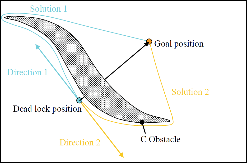
Fig. 5 shows the two feasible paths leading the robot to the goal position. Each path corresponds to one choice of the direction of the motion to follow the boundary of the obstacle. Therefore, and since the environment can be dynamic, the choice of the direction left or right is made once and it stays the same until the goal is reached. This unique choice guarantees a feasible path in all situations whenever a deadlock position is found by the local planner (even if in certain cases the choice seems to be non optimal).

Fig. 5.

If a solution exists any chosen direction will give a valid path

3.2. The n-dimensional case

In the case of a 3-DoF robot, the choice of a direction avoiding the obstacle becomes more complicated. Indeed, the directions perpendicular to the vector pointing toward the goal configuration are on a hyperplane of the CSpace, which is, in this case, a plane tangent to the obstacle and normal to the vector pointing to the goal position (fig. 6).

Fig. 6.

Plane of possible directions

This plane will be called TCplane (Tangent C plane). The path planner can choose any direction among those included in this plane. As in the case of 2-DoF case, we have no idea about the direction to choose in order to avoid the obstacle. In this case, an earlier method, proposed by Red et al. (Red, W.; Troung-Cao, H. & Kim, K., 1987), consists of using the 3D space made of the robots primary DoF. Then, by using a graphical user interface (GUI), the user moves the screen cursor to intermediate interference free points on the screen. A path is then generated between the starting and the final configurations going through the intermediate configurations.

This method is applicable only to the primary 3-DoF case when the 3D graphical model can be visualized. Also, the user can chose paths using only the primary DoF, which eliminates other possibilities using the full DoF of the robot. Moreover, this method cannot be applied in real time applications.

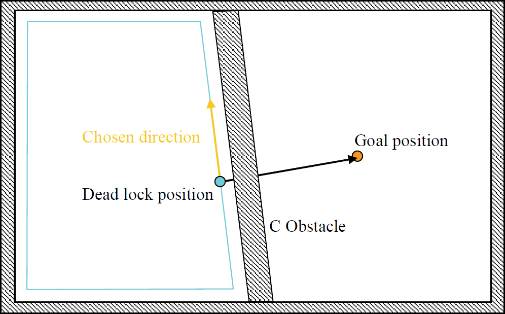
One possible strategy is to make a random choice of the direction to be followed by the robot in the TCplane. This strategy can lead to zigzagged paths and therefore should be avoided. In our case, whenever the robot is in a deadlock position, we make it evolve toward its upper joint limits or lower joint limits, defined by the vector q_lim. This strategy allowed us to find a consistent way to get out of the deadlock position. This chosen direction is defined by the intersection of the TCplane and the bypassing plane (P) containing the three points: q_lim, q_lock and q_goal (fig. 7).

Fig. 7.

Plane used to bypass the C Obstacle

In the general case of robots with many DoF, the TCplane is now a hyperplane which is normal to the vector pointing from q_lock to q_goal and containing q_lock. The direction chosen to go around the obstacle is defined by the intersection of the TCplane and the plane (P) defined by the three points: q_lim, q_lock and q_goal. New constraints, reducing the motion of the robot to the plane (P), are defined with respect to non collision constraints. The boundary following method will follow these constraints until the obstacle is avoided. This plane (P) will be characterized by two vectors U₁ and U₂, where U₁ is the vector common to all possible subspaces pointing out to the goal configuration. U₁ is given by:

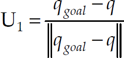
\begin{aligned} U_{1} = \frac{q_{g o a l} - q}{∥ q_{g o a l} - q ∥} \end{aligned}

(10)

U₂ is the vector that defines the direction used by the robot in order to avoid the obstacle. Let V be a vector given by:

\begin{aligned} V = \frac{q_{\lim} - q}{∥ q_{\lim} - q ∥} \end{aligned}

(11)

Where q_lim = q_inf if the chosen strategy makes the robot move toward the lower limits of its joints, and q_lim = q_sup if the chosen strategy makes the robot move toward the upper limits of its joints.

U₂ is the unit vector orthogonal to U₁ and located in the plane (U₁, V) (fig. 8). U₂ is given by:

\begin{aligned} U_{2} = \frac{V - (U_{1}^{T} V) U_{1}}{∥ V - (U_{1}^{T} V) U_{1} ∥} \end{aligned}

(12)

Fig. 8.

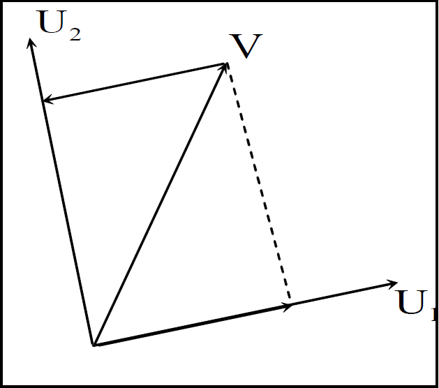
Definition of the vector U₂

While avoiding the obstacle, the robot will move in the defined subspace (P), and Δq could be written as

\begin{aligned} Δ q = Δ u_{1} U_{1} + Δ u_{2} U_{2} \end{aligned}

(13)

Where, Δu₁ is the motion along the U₁ direction and Δu₂ is the motion along the U₂ direction.

Whenever an object is detected by the robot, which means that the distance between the robot and the object is less then the influence distance, a constraint is created according to equation (7). Constraints are numbered such that the i ^th constaint is written as:

\begin{aligned} [a_{i 1} \dots a_{i N}] [Δ q_{1} \dots Δ q_{N}]^{T} \leq b_{i} \end{aligned}

(14)

If we replace Δq by its value in the subspace, we get

\begin{aligned} [a_{i 1} \dots a_{i N}] (Δ u_{1} U_{1} + Δ u_{2} U_{2}) \leq b_{i} \end{aligned}

(15)

\begin{aligned} a u_{i 1} = [a_{i 1} \dots a_{i N}] U_{1} \end{aligned}

(16)

\begin{aligned} a u_{i 2} = [a_{i 1} \dots a_{i N}] U_{2} \end{aligned}

(17)

The projected constraints are written as

\begin{aligned} A_{i}^{T} Δ u \leq b_{i} \end{aligned}

(18)

with

\begin{aligned} A_{i} = [a u_{i 1} a u_{i 2}]^{T} \end{aligned}

(19)

\begin{aligned} Δ u = [Δ_{u 1} Δ_{u 2}]^{T} \end{aligned}

(20)

In order to escape from deadlocks, we follow the projected constraints corresponding to the obstacles blocking the robot. To do so, we use the Boundary following method described in the next section.

3.3. The boundary following Algorithm

This method uses the the distance function defined as:

\begin{aligned} V (q) =∥ q - q_{g o a l} ∥ \end{aligned}

(21)

which is the distance from the current position of the robot to the goal position. The value of the distance function is strictly decreasing when the robot is evolving toward its goal using the local planner. When a deadlock is detected, we define d_lock = ‖q_lock – q_goal‖ as the distance function in the deadlock configuration. While the robot is going around the obstacles using the boundary following method, the distance function, V(q), is continuously computed and compared to d_lock. When the value of the distance function is lower than d_lock, the robot has found a point over the C obstacle boundary that is closer to the goal than the deadlock point. At this moment, the robot quits the boundary following method and continues to move toward the goal using the local planner. The vector of the followed constraint is named A _lock it corresponds to the vector of the projected constraint blocking the robot. The boundary following method can be stated as follows

Initiate the parameters A _lock and d_lock

Evaluate the distance function. If it is less than d_lock quit the boundary following method and resume the local planner

Find and update the followed constraint A _lock

Find the vertex enabling the robot to go around the obstacle

Move the robot and go to step 2

Fig. 9 shows the followed vertex Δu. It is the point on the constraint A _lock in the direction of S and it satisfies all the projected constraints.

S = [- {a u}_{l o c k 2} {a u}_{l o c k 1}]

(22)

Fig. 9.

Boundary following result

Where

\begin{aligned} A_{l o c k} = [a u_{l o c k 1} a u_{l o c k 2}]^{T} \end{aligned}

(23)

At each step the algorithm tracks the evolution of the followed constraint among the set of the projected constraints. The tracked constraint is the one maximizing the scalar product with A _lock .

In certain cases the resultant vertex Δu is null when there is another projected constraint blocking the robot (fig. 10). This is the case of point B in fig. 11. The robot switches the followed constraint. It uses the blocking constraint to escape from the deadlock.

Fig. 10.

Constraint switching

Fig. 11.

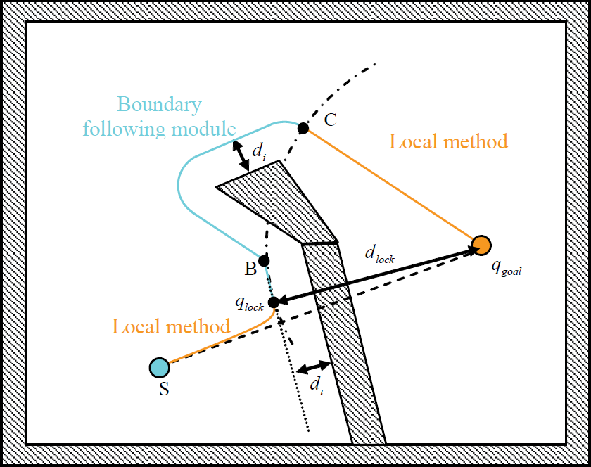
Illustrating example

Fig. 11 shows the case of a point robot moving from point S to point q_goal. The robot moves from point S to point q_lock1 using the local planner. The point q_lock1 corresponds to a deadlock position where the robot can no longer move toward the obstacle while respecting the security distance, d_s, from the obstacle. This point corresponds also to a local minimum of the distance function, V(q) = d_lock1. At this point, the robot starts to follow the boundary of the blocking obstacle and the distance function V(q) will continuously be compared to d_lock1. In point B there is another obstacle preventing the robot from following the first one. In that case, the boundary following module changes the path of the robot to follow the new obstacle. In point C the distance to the goal has decreased and becomes equal to d_lock1, which means that the robot avoided the obstacle and the local planner is resumed. When reaching point q_lock2, a second deadlock position occurs.

Therefore, the boundary following module is activated again until point D is reached, which corresponds to a distance from the goal equal to d_lock2. At this point the local method is resumed to drive the robot to its goal position.

4. Simulation and results

In order to evaluate the efficiency of the method, we present several examples. All the simulations have been performed on a robotic-oriented-Software named SMAR (Zeghloul, S.; Blanchard, B. & Ayrault, M. 1997).

This software is made of two modules: a modeling module and a simulation module. The modeling module is used to generate a model of the robots in their environment. The simulation module is used to simulate the motion of the robots and the obstacles. This method was added to the simulation module. All the following examples were simulated on a Pentium III 1.2 Ghz. Path planning was performed in real time and did not slow the motion of the robot compared to the case without obstacles.

The first example is made of a single 5-DoF robot in a cluttered environment (fig. 12). The ladder shaped obstacle does not allow the object to go through it, unless it is set in an appropriate orientation. In doing so, the robot follows the boundary of the obstacle until it gets in a configuration where there is no risk of collision and the local planner takes over the control of the robot to drive it safely to its goal position. These results can not be reached by using only the local planner.

Fig. 12.

Results using 5-DOF robot in a cluttered environment

The second example is made of two 5-DoF robots each one of them is taking an object from one initial position to a final one (fig. 13). In doing so, the two robots come closer to each other and they have to avoid collision. Frames 4, 5 and 6 show the two robots following the boundary of each other by keeping the security distance. This task would not be possible if we used only the local planner, because it would be stuck as soon as two faces of the two objects become parallel, which is happening in Frame 3.

Fig. 13.

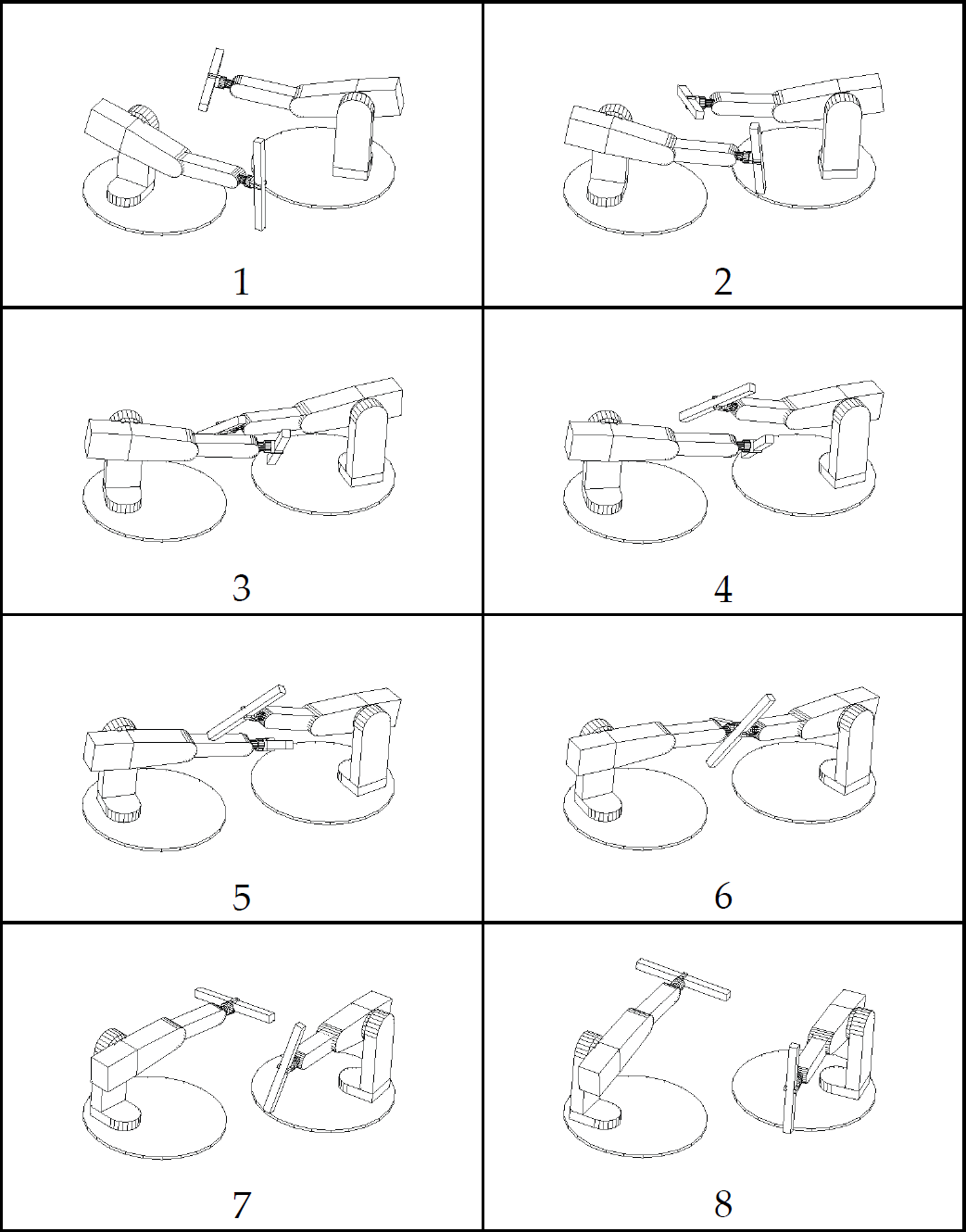
Results using two 5-DOF robots

Fig. 14 shows the results using three PUMA robots. Each one of the three robots considers the two others as moving obstacles. Each robot moves toward its goal, once a deadlock position is detected, the robot launches the boundary following method. Until Frame 3 the local planner is active for the three robots. As soon as the robots get close to each others the boundary following module becomes active (Frame 4).

Fig. 14.

Results using three PUMA robots

When each robot finds a clear way to the goal the local planner takes over (Frame 13) to drive each robot to its final position.

In these simulations, robots anticipate the blocking positions. If the module of the joint velocity given by the local method is less than 30% of the maximum joint velocity, the robot starts the boundary following method. Elsewhere, the boundary following method is stopped and local method is resumed when the distance function is less then 80% d_lock.

These values are found by performing some preliminary simulations. Anticipating the deadlock position makes the resultant trajectories smoother, as the robot does not wait to be stopped by the deadlock position in order to begin the boundary following method.

5. Conclusion

This work presents a novel method for path planning suitable for multi-DoF robots. This method is a combination of the classical local method and the boundary following method needed to get out the robot from deadlock positions in which the local method gets trapped.

The local path planner is based on non-collision constraints, which consist of an optimization process under linear non-collision constraints. When a deadlock is detected, corresponding to a local minimum for the local method, a boundary following method is launched. Similar method can be found for 2D cases, and we show in this work how it can be applied to the case of multi-DoF robots. When the robot is stuck in deadlock position, we define the direction of motion of the robot, in the configuration space, as the intersection of a hyperplane, called TCplane, and a plane defined by the vector to its goal and a vector to its joint limits. This direction of motion allows the robot to avoid the obstacle by following its boundary until it finds a path to the goal which does not interfere with the obstacle. Starting from this point the classical local planner takes over to drive the robot to its goal position.

This method is fast and easy to implement, it is also suitable for several cooperating robots evolving in dynamic environments.

References

Bohlin

& Kavraki

(2000). Path planning using lazy prm, Proceedings of IEEE International Conference on Robotics and Automation, pp. 521–528, San Francisco, CA, April 2000.

Faverjon

& Touranssoud

(1987). A local based approach for path planning of manipulators with a high number of degrees of freedom, Proceedings of IEEE International Conference on Robotics and Automation, pp. 1152–1159, Raleigh, March 1987.

Helguera

& Zeghloul

(2000). A local-based method for manipulators path planning in heavy cluttered environments, Proceedings of IEEE International Conference on Robotics and Automation, pp. 3467–3472, San Francisco, CA, April 2000.

Kavraki

Svestka

Latombe

J-C.

& Overmars

(1996). Probabilistic roadmaps for path planning in high dimensional configuration spaces. IEEE Transactions on Robotics and Automation, Vol. 12, No. 4, (august 1996), pp. 566–580, ISSN 1042-296X

Khatib

(1986). Real time obstacle avoidance for manipulators and mobile robots. The International Journal of Robotics Research, Vol. 5, No. 1, (1986), pp. 90–99

Kondo

(1991). Motion planning with six degrees of freedom by multistrategic bidirectional heuristic free-space enumeration, Proceedings of IEEE International Conference on Robotics and Automation, pp. 267–277, Sacramento, CA, April 1991.

Lengyel

Reichert

Donald

& Greenberg

(1990). Real-time robot motion planning using rasterizing computer graphics hardware. Computer Graphics, Vol. 24, No. 4, (August 1990), pp. 327–335

Lozano-Pérez

& Wesley

(1979). An algorithm for planning collision-free paths among polyhedral obstacles. Communications of the ACM, Vol. 22, No. 10, (October 1979), pp. 224–238, ISSN 0001-0782

Mediavilla

Gonzalez

Fraile

& Peran

(2002). Reactive path planning for robotic arms with many degrees of freedom in dynamic environments, Proceedings of 15 th Triennial Word Congress, Barcelona, Spain, 2002.

10.

Paden

Mess

& Fisher

(1989). Path planning using a jacobian-based free space generation algorithm. Proceedings of IEEE International Conference on Robotics and Automation, pp. 1732–1737, Scottsdale, Arizona, 1989.

11.

Ramirez

& Zeghloul

(2000). A new local path planner for nonholonomic mobile robot navigation in cluttered environments, Proceedings of IEEE International Conference on Robotics and Automation, pp. 2058–2063, San Francisco, CA, April 2000.

12.

Rao

S.S.

(1984). Optimization theory and applications, Wiley, ISBN 0470274832, New York

13.

Red

Troung-Cao

& Kim

(1987). Robot path planning in three-dimensions using the direct subspace. ASME Journal of Dynamics, Measurement and Control, Vol. 109, pp.238–244

14.

Siméon

Laumond

J-P.

& Nissoux

(2000). Visibility-based probalistic roadmaps for motion planning. Advanced Robotics Journal, Volume 14, No. 6, pp. 477–494, 2000, ISSN 0169-1864

15.

Yang

Simon X.

(2003). Biologically inspired robot behavior engineering, Biologically inspired neural network approaches to real-time collisionfree robot motion planning, pp. 143–172, Springer Verlag, ISBN 3790815136

16.

Skewis

& Lumelsky

(1992). Experiments with a mobile robot operating in a cluttered unknown environment, Proceedings of IEEE International Conference on Robotics and Automation, pp. 1482–1487, Nice, France, May 1992.

17.

Udupa

(1977). Collision Detection and Avoidance in Computer Controlled Manipulators, PhD thesis, Dept. of Electrical Engineering, California Institute of Technology, 1977

18.

Wilmarth

Amato

& Stiller

(1999). Maprm: A probabilistic roadmap planner with sampling on the medial axis of the free space, Proceedings of IEEE International Conference on Robotics and Automation, pp. 1024–1031, Leuven, Belgium, May 1999

19.

Zeghloul

Blanchard

& Ayrault

(1997). Smar: A robot modeling and simulation system. Robotica, Vol. 15, No. 1, (january 1997), pp. 63–73, ISSN 0263-5747