An On-Line Path Planner for Industrial Manipulators

Abstract

In this paper, an on-line path planner for an industrial manipulator is presented. The proposed control architecture is capable of driving the manipulator in its environment while avoiding collisions. Potential fields are used in order to control the joint velocities in such a way that the robot avoids the obstacles. We also propose a new weighted pseudoinverse matrix that improves the manipulator capability of finding feasible paths to move around obstacles and pass through narrow corridors without relying on the manipulator dynamic model. The proposed technique fits to both redundant and non-redundant manipulators. Experimental results show the effectiveness of the proposed solution.

1. Introduction

It is well-known that robotic manipulation is an established technology widely diffused in industry. Nevertheless, in recent years, the necessity for lean production makes it desirable to have robots with a certain degree of autonomy. In this context, the manipulator capability of autonomously taking some decisions by avoiding reprogramming off-line robot tasks each time is a key issue in the production process (e.g., replan the trajectory when moving pieces with different sizes).

Hence, developing a path planner capable of making a manipulator arm move in its environment by avoiding collisions is of significant concern. Bearing in mind that one of the goals is to avoid off-line reprogramming, a computationally light planner is desirable so that the trajectory can be modified at run time. Moreover, for an industrial robot, it is quite common to have very efficient and reliable velocity feedback control loops embedded in each motor drive and it is not always possible to open the velocity feedback control loops in order to directly control the motor torques. Thus, a purely kinematic control system whose output is a reference signal for each single motor velocity feedback control loop, instead of a torque signal, is preferable to implement in practical cases. Moreover, in this way, many local problems, such as friction compensation, are resolved in the motor inner control loops. Path planning and obstacle avoidance in a known environment have received much interest in recent years (see, for example, [LZR00, Vis00, DV03]). Many solutions have been proposed in the literature in order to solve these problems. They can broadly be divided into two main approaches: global strategies and local strategies.

The global solutions are commonly based on an off-line computation of a collision-free path from an initial configuration to the desired one [LP83, Lat91, LaV06]. Despite the desirable completeness property i.e., the capability of finding a feasible path in a finite amount of time (if it exists), these path planners are computationally heavy. Indeed, their computational burden exponentially increases with the number of manipulator degrees-of-freedom (DOF). For this reason, in view of the industrial requirement of on-line planning, they are far from being applicable.

Alternatives to the global approach are local techniques. They are less computationally demanding and thus preferred for on-line application. Basically, they are based on the definition of potential fields in the robot operational space. The obstacles are surrounded by repulsive potential fields and the goal position is represented by an attractive potential field. Hence, the potential fields push the manipulator links away from obstacles, thus avoiding collisions, while driving the manipulator end-effector toward the goal position. Even though local techniques are not complete, they are suitable for industrial applications. Indeed, it has to be considered that a typical industrial environment is not so complex (compared to typical research environments such as labyrinths or multidimensional bug traps) and can be well described via simple geometric shapes. As a matter of fact, in these kinds of environments, local techniques are capable of finding a feasible path while remaining far more suitable for computation.

Two different types of local techniques have been proposed in the literature. The first class is based on the joint torque control [Kha83, Kha86, VK90, ASZK98]. Artificial potential fields are used to exert virtual forces on the manipulator links (i.e., to control the joint torques). The main drawback of these solutions in view of an industrial application (besides the problems of torque controlled joints discussed above), is that they strongly rely on the manipulator dynamic model which is difficult to obtain in many practical cases. Indeed, it would require detailed information about each manipulator's mechanical component. This information, in many industrial contexts, is not fully available.

The second class of local techniques also uses the potential fields, but to calculate the joint velocity reference signals in order to reach the goal position along a collision-free path. In this context, the manipulator redundancy is exploited to avoid collisions by controlling the joint velocities in the manipulator nullspace [MK85, KK92, AHK93, CK96, ITZ⁺06, LWY09]. In these works, in order to let a certain point on the robot move at a given velocity, the Moore-Penrose pseudoinverse is used. This solution leads to unnatural manipulator behaviour reducing the manipulator capability of turning around obstacles [PP11]. Moreover, using the nullspace to avoid obstacles cannot completely ensure collision avoidance.

A different local approach is the dynamical system-based technique proposed in [KZB12a, KZB12b]. First, the dynamical system describing the manipulator behaviour is derived and then it is modified to avoid collisions. The system is modified accordingly to the given analytical functions describing the obstacles as smooth and non-convex surfaces. Even though these techniques seem promising, from an industrial point of view the derivation of a dynamic model seems difficult.

The solution proposed in this paper uses the potential fields in order to control the joint reference velocities. The collision avoidance control system acts on each link, even in the manipulator nullspace (i.e., to avoid collisions, the end-effector trajectory is also changed), making the proposed control system applicable to both redundant and non-redundant manipulators. The obstacle avoidance control system and the goal position following system are completely separate, as in the solution proposed in [Kha86] (where, on the contrary, joint torques were controlled). Nevertheless, the two systems are not decoupled, since not only the manipulator nullspace is used to avoid collisions, but also those vectors in the joint space that modify the end-effector trajectory.

In order to allow the proposed system work properly, a new pseudoinverse matrix is introduced. The computation of the new pseudoinverse only requires kinematic information (that is commonly known in industrial environments) and increases the manipulator capability of moving around obstacles. Both simulation and experimental results prove the effectiveness of the proposed solution.

The paper is organized as follows: in Section 2, the obstacle avoidance technique is presented, while the goal position following system is described in Section 3. The new weighted pseudoinverse is proposed in Section 4, and Section 5 is devoted to illustrative simulation examples. In Section 6, experimental results are presented, and conclusions are drawn in Section 7.

2. Obstacle avoidance

The proposed solution is aimed at making the manipulator autonomously navigate toward the goal end-effector position along a collision-free path. Being an on-line path planner, the path is not computed in advance, but at run time, while the manipulator is already executing the required task. Each link, when close to an obstacle, feels the virtual repulsive potential field surrounding the obstacle. This field is used to compute a reference signal for the joint velocity feedback control loops in order to make the link move away from the obstacle surface. Along the same line, the end-effector is pulled toward the goal position by making it move at a certain velocity depending on a given potential field surrounding the goal position. The desired end-effector velocity is then translated into reference signals for the joint velocity feedback control loops.

All the joint velocity terms are finally added. This means that the real end-effector velocity also depends on all the desired link velocities (to make them escape from obstacles) and vice versa.

It is worth stressing that once the desired operational space velocity for a certain point along the manipulator kinematic chain has been computed, this request can be fulfilled by using different joint velocities. Given a general point along the manipulator kinematic chain, we propose here a solution to choose the desired joint velocities in such a way that leads to good results, without involving the knowledge of the manipulator dynamic model.

2.1. Distance and repulsive potential fields

Even though this work is focused on the control system and the solution proposed in the following paragraph is rather general and does not depend on the way the distance and the potential field are defined, a brief discussion about distances and potential fields may help the reader to better understand the following sections. Please note that within the same control strategy, other potential fields and different notions of distance could be used instead of the ones proposed hereafter.

In the literature, several potential field formulations exist, but two main approaches have been proposed: it is possible to define the repulsive potential field using a superquadratic function [VK90] or a harmonic function [KK92]. Actually, using harmonic functions has a great advantage for mobile robots, since local minima are avoided. However, it is not very useful for manipulator arms where there are several points controlled by the potential fields, in addition, it is much more complex and computationally heavier. Indeed, it is worth noting that in the case of industrial manipulators, being in general relatively simple environments, it is quite unusual to get the end-effector trapped in a local minimum depending on the fields acting on it. On the contrary, it is more realistic to get the whole robot trapped in local minima depending on the superposition of the effects of the repulsive potential fields acting all along the manipulator kinematic chain and the effect of the attractive potential field acting on the end-effector (e.g., the manipulator is trying to surround an obstacle whose perimeter is longer than the manipulator kinematic chain). Bearing this idea in mind, we use here the well-known potential field proposed in [Kha 86]:

$\text{U(x)=}\{\begin{array}{cc}\frac{\text{kav}}{2}{\left(\frac{1}{\rho }-\frac{1}{\rho 0}\right)}^2& \text{if }\rho \le \rho 0\\ 0& \text{if }\rho >\rho 0\end{array},$

(1)

where k_av, ρ₀ and ρ are (respectively) a numeric constant, the limit distance of the potential field influence and the distance between a certain point where the potential fields is calculated and the obstacle. In order to calculate the desired velocity for a certain point I, we calculate the opposite of the potential field gradient at x = I:

$\dot{\mathrm{x}}\text{I=}-\nabla \text{U(x)}|{}_{\text{x=I}}.$

(2)

Evidently the concept of potential field is intimately related to the concept of distance. Indeed, in order to compute the effect of a given field on a given point along a given link, we must know the distance between the link and the obstacle surrounded by the field. However, calculating the distance between an obstacle and a manipulator link could be quite complex unless the geometry of the obstacle itself is relatively easy. But this is exactly the typical case of an industrial environment Moreover in many cases, instead of using the Euclidean distance, we can use a pseudodistance a approximating the obstacle shape with a superquadratic surface [Pas01, PPD02]. Furthermore using superquadratic surfaces to approximate the obstacle shapes, allows a fast and automatic computation of the distance between a given link and the obstacle

Note that the use of superquadratic surfaces may reduce the real feasible space. While this is a major drawback in the case of a mobile robot navigating in hypercluttered environments, from an industrial point of view this is acceptable and it actually increases the safety margins.

2.2. Control system

Now that a potential field and a method to compute the distance between obstacles and links (they are taken from the literature and they are not the only usable approaches) have been defined, we can describe the obstacle avoidance control system. In order to avoid collisions, the virtual potential fields are used to change the joint reference velocities. The repulsive fields act on some control points called psp, distributed along the manipulator kinematic chain. At each instant, the psp are dynamically computed as the nearest points between every link and every obstacle. Note that the calculation of the nearest point by using superquadratic surfaces to envelope the obstacles is an optimization problem whose outcome is an algebraic equation [Pas01, PPD02], so that this procedure can be completely automatized.

Figure 1.

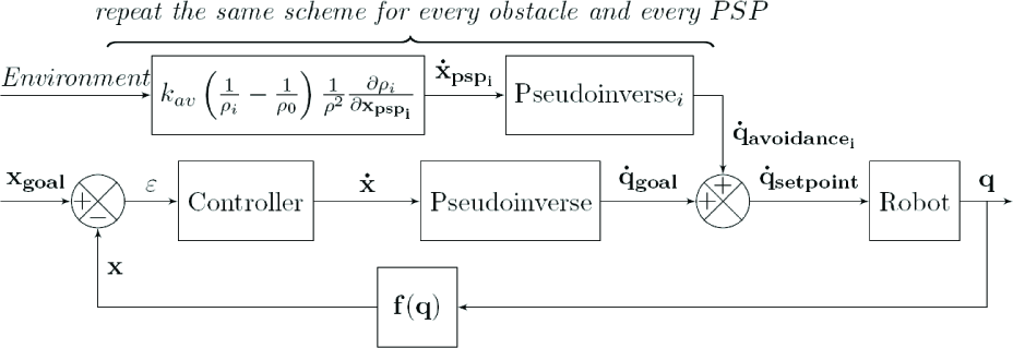
The control system block scheme.

As stated before, we use the repulsive field to control the manipulator joint velocities. Hence, each control point is a velocity controlled point whose desired velocity depends on the repulsive potential fields surrounding the obstacles according to (2). In order to calculate the desired velocity for the ith psp for a given obstacle, we apply (2) to (1) obtaining the following equation:

${\dot{\mathrm{x}}}_{\text{pspi}}=\{\begin{array}{cc}\text{kav}\left(\frac{1}{\rho \mathrm{i}}-\frac{1}{\rho 0}\right)\frac{1}{{\rho }_{\mathrm{i}}^2}{\frac{\partial \rho \mathrm{i}}{\partial \text{xpspi}}}^{}& \text{if }\rho \mathrm{i}\le \rho 0\\ 0& \text{if }\rho \mathrm{i}>\rho 0,\end{array}$

(3)

where k_av and ρ₀ are (respectively) the intensity of the repulsive potential field and the limit distance of the potential field influence (both parameters to be tuned); ρ_i is the distance between the ith control point and the obstacle.

In the case of multiple obstacles, the same procedure should be applied to every obstacle in the environment and for each control point.

Once the desired velocity for each control point has been computed, the requirement should be translated into desired joint velocities to be used as reference signals for the joint velocity loops. Given a single psp, the joint reference velocities can be obtained by means of a Jacobian pseudoinverse. Here, all the control points, at least one for each link, simultaneously generate joint velocity signals.

As it will be shown in the next section, the end-effector is controlled by a different system, called a goal position following system, that is used to compute the desired operational space velocity. This request, again, is translated via Jacobian pseudoinversion into a joint velocity additional term.

All the joint velocity terms are eventually added in order to obtain reference signals for the joint velocity feedback control loops. This solution is summarized by the control scheme represented in Figure 1.

It is worth stressing that because reference signals are finally computed as the summation of all the velocity terms generated from all the control points and from the end-effector, the actual velocity of a given point is different from the desired one. This approach guarantees obstacle avoidance because, if a given psp is really close to an obstacle, it is pushed away even if, in order to do that, the end-effector trajectory is perturbed.

Remark 1. This work is based on the hypothesis that a perfect joint velocity tracking is guaranteed. Note that this hypothesis is quite realistic, since in practical cases industrial robots have very fast and effective servomotors. Otherwise, even a simple planned task such as trajectory following would be infeasible.

3. End-effector control

In order to make the end-effector reach the goal position, two proportional controllers are used, one for the position x_p and another for the orientation x_a. Let x_goal be the goal generalized position (i.e., position and orientation) and x the end-effector generalized position in the operational space, defined as follows:

$\mathrm{x}=\left[\frac{\text{xp}}{\text{xa}}\right]=\left[\begin{array}{l}\mathrm{x}\\ \mathrm{y}\\ \mathrm{z}\\ -\\ \alpha \\ \beta \\ \gamma \end{array}\right].$

(4)

The position following controller is described by this simple equation:

$\dot{\mathrm{x}}\text{p=kv}\left({\mathrm{x}}_{{\mathrm{p}}_{\text{goal}}}-x_p\right),$

(5)

where k_v is a control parameter used to tune the controller.

For the end-effector orientation, a more complex solution has been developed. It is known that once two different configurations of a rigid body (i.e., the end-effector) are chosen, it is always possible to define a unique screw motion [MLS94] linking the two configurations. We can calculate two parameters: a translation d along the screw axis and a rotation ϑ around the screw axis will move the rigid body from the initial generalized position to the final one. We are only interested in the ϑ parameters: at each instant, we calculate the screw axis, since we know the actual position and the goal position. Then we calculate the desired angular velocity ω as a vector having the same direction of the screw axis and norm proportional to the angle ϑ. Let M be the homogeneous matrix describing the end-effector generalized position with respect to the base frame and M_goal the homogeneous matrix describing the generalized position x_goal. The above described screw motion is represented by the following matrix: Q = M_goalM⁻¹. It can be shown [MLS94] that the screw axis direction is represented by the following unit vector:

$\text{u=}\left[\begin{array}{l}{u}_x\\ u_y\\ u_z\end{array}\right]\text{=}\left[\begin{array}{l}\frac{{\mathrm{Q}}_{32}-{\mathrm{Q}}_{23}}{2\sin \vartheta }\\ \frac{{\mathrm{Q}}_{31}-{\mathrm{Q}}_{13}}{2\sin \vartheta }\\ \frac{{\mathrm{Q}}_{21}-{\mathrm{Q}}_{12}}{2\sin \vartheta }\end{array}\right].$

(6)

where ϑ is calculated as follows:

$\begin{array}{l}\mathrm{c}=\frac{{\mathrm{Q}}_{11}+{\mathrm{Q}}_{22}+{\mathrm{Q}}_{33}}{2},\\ \mathrm{s}=\pm \frac{\sqrt{{\left({\mathrm{Q}}_{32}-{\mathrm{Q}}_{23}\right)}^2}+{\left({\mathrm{Q}}_{31}-{\mathrm{Q}}_{13}\right)}^2+{\left({\mathrm{Q}}_{21}-{\mathrm{Q}}_{12}\right)}^2}{2},\\ \vartheta =\text{a tan2(s},\text{c)}\end{array}$

(7)

Note that (6) may become singular (e.g., when the pitch of the skew motion is null). In these cases the screw axis can be computed using different formulae [MLS94, Leg00]. Now we have all the necessary information to build the orientation following controller:

$\omega =\text{kw}\vartheta u\text{,}$

(8)

where k_w is a control parameter for tuning the orientation controller.

Using this equation and (5), we describe the whole end-effector position controller as follows:

$\dot{\mathrm{x}}=\left[\begin{array}{c}\dot{\mathrm{x}}\mathrm{p}\\ \omega \end{array}\right]\text{=}\left[\begin{array}{c}{k}_v\left({\mathrm{x}}_{{\mathrm{p}}_{\text{goal}}}-x_p\right)\\ \mathrm{k}\omega \vartheta \mathrm{u}\end{array}\right].$

(9)

The previous equation is simply addressed as controller in Figure 1, and is represented like a unique block scheme. Note that this solution exactly corresponds at having a quadratic attractive potential field (a paraboloid) defined around the goal position and ϑ.

However, this goal position following system, when using fixed control parameters, presents some problems. In fact, an aggressive tuning, when the end-effector is far from the goal configuration, leads to excessive joint velocities. On the other hand, a parameter detuning would lead to a sluggish controller and consequently the robot would take a lot of time to reach the goal configuration.

To overcome this problem, it is possible to increase the coefficients k_v and k_w when the endeffector is close the goal configuration. In order to do that, we propose a gain scheduling system that tunes the parameters at run time.

This solution has been already used in the literature [ZVL 06].

3.1. Gain scheduling

Let k_v0 and k_w0 be the initial values of the control parameters, ρ₀ the initial distance between the end-effector and the goal position and ρ the distance between the end-effector and the goal position. We can tune up the parameters as follows:

$\begin{array}{l}\text{if}\frac{\rho 0}{\rho }<\upsilon \text{max}\\ \text{ kv}=\text{kv}0\frac{\rho 0}{\rho },\\ \text{ kw}=\text{kw}0\frac{\rho 0}{\rho }.\end{array}$

(10)

The control parameters are anyway bounded by using the v_max value in order to avoid instability. Using this simple solution allows us to obtain better results, namely, a lower time to execute the task and bounded motor velocities.

In particular, regarding the motor velocities, there is a safety threshold q̇_max in order to avoid excessively stressing the joint motors. If a single motor crosses the maximum allowed velocity threshold (in absolute value), the whole vector q̇ is reduced by multiplying it by this ratio: $\frac{\dot{\mathrm{q}}\text{max}}{\max \left(\left|\dot{\mathrm{q}}\right|\right)}$ . Using this solution, we do not change the end-effector velocity direction, but only the intensity, thus we do not change the path.

4. Weighted pseudoinverse

In order to make the proposed control architecture work properly, an effective pseudoinverse of the kinematic model is needed. In particular, because the control points are generally distributed along the kinematic chain, and not located at the end of it, we are completely free to decide how to move the joints between a given psp and the end-effector. Moreover, since the manipulator can be redundant, even when controlling the end-effector, we may have free movements in the joint space. We propose here a solution to address this problem after showing that the classical choice of using the Moore-Penrose pseudoinverse leads to poor results, making the manipulator moving in an unnatural manner.

Let n be the number of manipulator DOFs, P a certain point on the kth link, with k ≤ n and ẋ, am × 1 vector, the desired velocity for the point P (with m ≤ n).

The most diffused solution in the literature is the classical Moore-Penrose pseudoinverse: let J be the Jacobian matrix of the P point, J is amxnmatrix defined as follows:

$\text{J(q)=}\left[\begin{array}{cccccc}\frac{\partial \mathrm{x}1}{\partial \mathrm{q}1}& \cdots & \frac{\partial \mathrm{x}1}{\partial \text{qk}}& 0& \cdots & 0\\ ⋮& & ⋮& ⋮& & ⋮\\ \frac{\partial \text{xm}}{\partial \mathrm{q}1}& \dots & \frac{\partial \text{xm}}{\partial \text{qk}}& 0& \cdots & 0\end{array}\right]$

(11)

The Moore-Penrose pseudoinverse is then defined as:

${\mathrm{J}}^{†}=J^T{\left({\text{JJ}}^{\mathrm{T}}\right)}^{-1}$

(12)

This solution minimizes the joint velocity Euclidean norm ||q̇||, thus the joints far from P toward the robot base are moved faster than the nearer ones, while, as shown in Figure 2, the joints from k to n are kept rigid.

The consequence of this behaviour is that bigger joint torques are required because the joints toward the manipulator base see bigger inertiae. Evidently, this is not desirable in an industrial perspective considering that it means increased energy consumption and components stress. Moreover, an unnatural manipulator behaviour is obtained because the joints between the considered P and the end-effector are kept blocked. In particular, the second problem is the most important one: it is frequently needed to make the manipulator turn around an obstacle to find the goal position, or pass through a narrow corridor between two obstacles moving around the obstacles to avoid collisions. When using the Moore-Penrose pseudoinverse, the manipulator escapes the P point from the obstacle moving also the end-effector like a rigid body. This behaviour (see Figure 3) strongly reduces the path planner capability of finding a feasible path toward the goal position.

A primary idea to overcome this problem could be to use a weighted pseudoinverse, using the manipulator mass matrix like a metric. This solution would minimize the kinetic energy, thus leaving the last n-k joints unactuated.

However, this solution needs a complex dynamic model including all the link dynamic parameters to be developed, thus, for the reasons discussed in the previous sections, it is not suited for industrial applications.

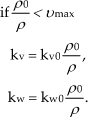
In order to avoid the dynamic model definition, which requires a lot of information on the robot mechanical structure, we have developed a weighted pseudoinverse that leads to suitable results without involving the knowledge of the manipulator dynamic properties, as Figure 2 and Figure 4 show. In order to create the weighted pseudoinverse, we define a 3n × 3n diagonal matrix W (2n × 2nfor a planar manipulator) whose diagonal terms correspond to the elements of a vector w.

$\text{W=}\left[\begin{array}{ccccccc}\mathrm{w}1& & & & & & \\ & \mathrm{w}1& & & & & \\ & & \mathrm{w}1& & & & \\ & & & \ddots & & & \\ & & & & \text{wn}& & \\ & & & & & \text{wn}& \\ & & & & & & \text{wn}\end{array}\right]$

(13)

Figure 2.

The manipulator behaviour using different pseudoinverse Jacobian matrices.

Figure 3.

The manipulator fails turning around the obstacle to pass through a narrow corridor using the Moore-Penrose pseudoinverse.

Now we define the following matrix J_e relating to the Cartesian velocity of each joint (seen like a point in the space) and of the end-effector with the joint velocities. Since we know the manipulator geometry, it is always possible to calculate this matrix. This is a 3n × n matrix (2n × n for a planar manipulator) defined as follows:

$\text{Je=}\left[\begin{array}{ccc}\frac{\partial {\text{xjoint}}_1}{\partial \mathrm{q}1}& \cdots & \frac{\partial {\text{xjoint}}_1}{\partial \text{qn}}\\ ⋮& \ddots & ⋮\\ \frac{\partial \text{zjointnn}}{\partial \mathrm{q}1}& \cdots & \frac{\partial \text{zjointnn}}{\partial \text{qn}}\end{array}\right]$

(14)

By means of (14), we are ready to define the weight matrix:

$\mathrm{G=}{J}_e^{T}W{J}_e$

(15)

This is actually a simplified mass matrix, like the one describing the dynamics of a robot whose masses [w₁ … w_n] are concentrated at the joints at the end of every link (from 1 to n-1) and at the end-effector (n).

The new proposed pseudoinverse is then defined by using the G matrix as a metric:

$\tilde{J}=G^{\mathrm{-1}}{J}^T{\left(J{G}^{\mathrm{-1}}{J}^T\right)}^{\mathrm{-1}}$

(16)

Eventually, we choose the solution that minimizes the virtual kinetic energy of a robot whose mass matrix is G.

This can be proven using the Lagrange multipliers. Indeed, let O=1/2q̇G(q)q̇ be the optimization function, i.e., the virtual kinetic energy, and C=ẋ-J(q)&qdot; = 0 the equality constraint. We can write the Lagrangian equation as follows:

$\text{L=O+}{\lambda }^T\mathrm{C},$

(17)

where λ is the Lagrange multiplier vector. Differentiating the previous equation with respect to q̇ and λ, we obtain the following system

$\{\begin{array}{l}\frac{\partial \mathrm{L}}{\partial \dot{q}}\mathrm{=G}\left(q\right)\dot{q}-{\mathrm{J}}^T\lambda =0\\ \frac{\partial \mathrm{L}}{\partial \lambda }=\dot{\mathrm{x}}-J\dot{\mathrm{q}}\text{=0}.\end{array}$

(18)

(16) follows straightforwardly solving the system.

Using this pseudoinverse, we force the manipulator to move in the same way a kinematic chain having all the masses localized at the joints at the end of the links and at the endeffector would do, pushed at the P point when we assume null joint torques (see Figure 2).

The w vector is a control parameter, the bigger a certain term w_i is, the more the control system moves slowly the i-th link in order to get the same Cartesian space velocity. Indeed, it means the ith virtual link is heavier and is therefore moved slowly to minimize kinetic energy. When a link at the middle of the manipulator kinematic chain approaches an obstacle, it is pushed away. The proposed pseudoinverse minimizes the virtual kinetic energy so that the obstacle avoidance controller does not actuate the joints between the link close to the obstacle and the end-effector. In this way, this part of the kinematic chain remains completely driven by the end-effector controller that makes the robot bend around the obstacle, improving its capability of turning around obstacles. Now consider the case of one of the terminal links approaching an obstacle. To push away from the obstacle a point along this link, the weighted pseudoinverse strongly moves the last joints and barely actuates the first ones. In this way, the last links turn along the obstacle surface, allowing the manipulator to reach the opposite side of the obstacle. A clear example of both these behaviours can be seen in subsection 5.3. Summarizing, the weighted pseudoinverse avoids the obstacle avoidance system and the end-effector controller to work one against the other.

A simple and effective choice is to set every element of w equal to one, that means that every link has the same virtual mass. This is an effective solution, as it will be shown in the next sections.

It is worth noting again that this solution never involves the knowledge of the robot dynamic parameters and the calculation of the dynamic model.

Figure 4.

The manipulator successfully turns around the obstacle to pass through a narrow corridor using the weighted pseudoinverse.

5. Simulation examples

Several simulations have been performed, in order to test the effectiveness of the proposed technique before implementing it on a real industrial manipulator. In particular, the obstacle avoidance capability has been tested. We tested the capacity of dealing with redundancy with both planar and spatial manipulators, the capability of driving the manipulator through narrow passages and the effect of the weighted pseudoinverse and of the gain scheduling system. During these simulations a perfect joint velocity tracking has been considered. The experimental results proposed in the next section will prove that this assumption is indeed realistic when dealing with industrial servodrives.

5.1. Example 1: Obstacle avoidance

The control system has been first tested on a seven DOF spatial manipulator arm, with the same kinematic structure of the Motoman IA20 robot. This manipulator, as shown in Figure 5, can be seen like two spherical robots, the first three joints and the last three joints (spherical wrist) coupled with a joint (the fourth one) located between the two sphere centres.

Figure 6 shows a simple example of obstacle avoidance: the control system is able to make the manipulator avoid the collision turning around the obstacle.

5.2. Example 2: Narrow passages

As a second simulation, the path planner is required to make the same spatial manipulator move between two ellipsoidal obstacles. Figure 7 shows the capability of the control system to avoid collisions and to pass inside the corridor between the two obstacles. The path planner drives the end-effector, avoiding at the same time collisions between all the manipulator links and the obstacles.

5.3. Example 3: High redundancy

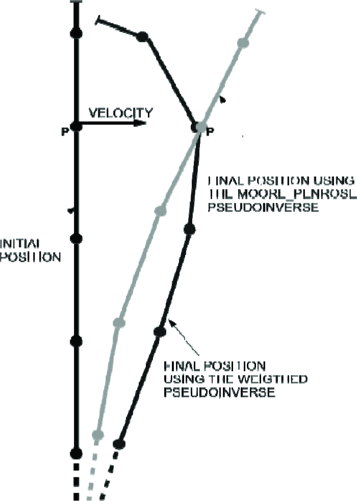
In order to test the capability of dealing with high redundant structures, a seven DOF planar manipulator has been simulated. The robot environment is cluttered with multiple obstacles. The simulation proves the capability of the proposed control system to deal with hyper redundant manipulators, turn around obstacles and deal with several obstacles as shown in Figure 8.

5.3. Example 4: Weighted pseudoinverse

We have also tried to execute the same task of the previous simulation, but using the MoorePenrose pseudoinverse instead of the weighted one we have proposed. Without the weighted pseudoinverse, the path planner fails: it cannot drive the end-effector to the goal position.

Figure 5.

The kinematic scheme of a Motoman IA20 manipulator.

Figure 6.

An example of obstacle avoidance with a 7R IA20 spatial manipulator.

Figure 7.

Capability of passing through narrow passages while moving in three dimensional space.

Figure 8.

The path planner is able to drive the manipulator at the goal position using the weighted pseudoinverse.

Figure 9 shows that the manipulator cannot find a feasible path.

5.4. Example 5: Gain scheduling

Finally, we have simulated the same task, the first time with fixed control parameters, the second time using the gain scheduling proposed in this paper. In order to test the gain scheduling effect in depth, we have executed the task keeping the maximum joint velocity bounded under 17 rad/s.

Using the gain scheduling, we have strongly detuned the control parameters (more than 50% less) in order to have lower velocities at the beginning of the task execution. We have also reduced the time needed to complete the same task by more than half (see Figure 10 and Figure 11). This happens because, using the gain scheduling, we have higher velocities when we are already close to the goal configuration.

6. Experimental results

The results shown in the previous section have demonstrated the effectiveness of the proposed solution. In order to have a full confirmation of this, we have tested the proposed solution on a real manipulator. The considered robot is the two DOF planar parallel machine shown in Figure 12. The geometrical characteristics of the robot are reported in Table 1 (refer to Figure 12). As Figure 12 shows, the robot has been heavily loaded with a 10 [kg] mass, mounted on the manipulator end-effector (the P point). On the contrary, the links are made of very light aluminium bars, so that their masses can be safely neglected.

The joints are actuated with a couple of brushless servomotors through a couple of epicycloidal speed reducers. The maximum motor continuous torque is T_max = 3[Nm], while the maximum peak one is T_peak=6[Nm]; the speed reduction ration is i = 10 and the speed reducer mechanical efficiency is η = 0.95 (note that epicycloidal speed reducer has a very symmetrical behaviour between direct and reverse motion). The global momentum of inertia of motor rotor and speed reducers is I = 0.66[kgcm²]. Note that it cannot be neglected because, due to the speed reducer effect, its dynamic behaviour is increased i² = 100 times on the manipulator dynamic.

Table 1.

Manipulator link lengths.

Link	Length
l0	14[cm]
l1	5[cm]
l2	14[cm]
l3	14[cm]
l4	5[cm]

Figure 9.

The path planner fails using the Moore-Penrose pseudoinverse.

Figure 10.

Joint velocities without the gain scheduling.

Figure 11.

Joint velocities using the gain scheduling.

Figure 12.

The industrial robot and its kinematic scheme.

In this context, the aim of loading the end-effector is to test the control system under strongly coupled inertial behaviours (note that they are typical of robotic systems). Indeed, without the load, the manipulator dynamic would be dominated by the motors' inertia, leading to a simple decoupled behaviour. Figure 12 also shows that the manipulator works in the vertical plane. Hence, the servomotor velocity loops also have to compensate the gravity force. In this framework, a successful result would testify to the effectiveness of the choice of using the inner joint velocity loops in order to drive the robot in its environment.

The velocity control loops are embedded into the servomotor drives - they receive the joint reference velocity signals via the real-time Ethernet bus Powerlink (see [Aut] for details) from the Programmable Logic Controller (PLC). The control algorithm is implemented in the real-time operative system Automation Runtime (see [Aut] for details) that runs on the PLC accordingly to the PLCopen standard [PLC]. The control cycle is of 0.8 [ms], so that the velocity reference signals are refreshed with the same frequency.

It is worth stressing that all the components employed are off-the-shelf products [Aut]. This proves that the proposed technique is indeed suitable for industrial applications. A circular obstacle is placed in the manipulator operational space as Figure 13 shows. The considered obstacle size is a circle whose diameter is of 7 [cm] and its centre is at the position x = 0[cm], y = 12.8[cm]; see Figure 14. It is worth stressing that this measure is bigger than the actual obstacle size because the end-effector size also has to be considered in order to avoid collisions. Note that considering a bigger obstacle (increase of the load size) and an ideal (a point) end-effector, or the real obstacle and the real (with the load size) end-effector, leads to the same results.

The robot is required to reach three points in its operational space, represented by the coloured diamonds in Figure 14, where also the ideal (obstacle free) and the actual trajectory are shown. The first set of tuning parameters has been chosen with k_av =0.08 and k_v =0.5 (note that here, having a two DOF robot, k_w is not needed). The gain scheduling parameter has been chosen such that the gain can increase at most ten times its initial value, i.e., v_max = 10. The minimum distance under which the potential field starts acting on the manipulator is ρ₀=1[cm].

The proposed path planner successfully drives the end-effector to all the goal positions moving around the obstacles as shown in Figure 14. It is worth noting that, as shown in Figure 15, despite the big load and the gravity, the actual velocities and the reference ones are practically undistinguishable, except for the small noise due to numerical differentiation of the encoder signals.

In order to analyse the proposed solution in depth, a more aggressive tuning has been tested, increasing both k_av and k_v ten times. The results are reported in Figure 16. The time required to execute the task is greatly reduced, but again, despite the increased dynamics, the velocity tracking error is small.

It is interesting to note that when strongly increasing the tuning parameter, the manipulator exhibits an underdamped behaviour when it is very close to the obstacle, because of the strong potential field that locally behaves like a stiff spring.

Figure 13.

The obstacle in the robot environment.

Figure 14.

The obstacle (black line), the obstacle-free trajectory (blue line) and the actual trajectory (red line).

Figure 15.

The actual joint velocities (red and green lines) and the reference joint velocities (black lines) with the first set of tuning parameters.

Figure 16.

The joint actual velocities (red and green lines) and the joint reference velocities (black lines) with the second set of tuning parameters.

7. Conclusions

In this paper, a path planner suitable for industrial applications has been proposed. It is capable of driving the manipulator in a cluttered environment toward the desired position while avoiding collisions.

The proposed technique is computationally light and solely based on the robot kinematic model. Hence, it is suitable for on line applications and does not require the manipulator dynamic model. This solution is thus very useful when, as is usual in industrial contexts, it is difficult to model the manipulator dynamics or to control the joint torques.

The proposed solution works properly both with redundant and non-redundant manipulators.

A new pseudoinverse Jacobian has been proposed in order to solve the inverse kinematic problem for several points along the manipulator kinematic chain. Using the weighted pseudoinverse, the manipulator capability of turning around obstacles and moving in narrow passages is increased.

Once a potential field formulation was chosen, we tested the control system on both planar and spatial redundant manipulators with successful results.

Finally, the proposed solution has been experimentally tested on a real industrial robot by implementing the algorithm on a motion control industrial PLC driving two industrial brushless servomotors. The obtained results confirm its effectiveness. It is remarkable that the performance remains satisfactory also when the control parameters span over a wide range.