Sage Journals: Discover world-class research

Abstract

A distributed control algorithm based on a stimulus pulse signal is proposed in this paper for the locomotion of a Modular Self-reconfigurable Robot (MSRR). This approach can adapt effectively to the dynamic changes in the MSRR's topological configuration: the functional role of the configuration can be recognized through local topology detection, dynamic ID address allocation and local topology matching, such that the features of the entire configuration can be identified and thereby the corresponding stimulus signals can be chosen to control the whole system for coordinated locomotion. This approach has advantages over centralized control in terms of flexibility and robustness, and communication efficiency is not limited by the module number, which can realize coordinated locomotion control conveniently (especially for configurations made up of massive modules and characterized by a chain style or a quadruped style).

Keywords

Modular Self-reconfigurable Robot Coordinated Locomotion Distributed Control Stimulus Pulse

1. Introduction

The Modular Self-reconfigurable Robot (MSRR) plays a significant role in robotics: it is a complex distributed system composed of multiple modular cells. It can achieve transformations between configurations and realize locomotion by changing the connection styles between the modules in order to adapt to distinctive environmental requirements or else to execute different tasks [1]. MSRR is featured by adaptability, versatility and flexibility, etc. Modules in a self-reconfigurable robot must collaborate and synchronize their actions in order to accomplish desired global effects [2]. Possible applications of an MSRR include: a reconfigurable robot could change its shape into a snake to get through narrow places during a rescue operation, then into a quadruped to carry a load, or it may split into many smaller robots in order to perform a task in parallel. Many scholars have begun to investigate this research domain [3 –10] and have designed and implemented many systems, as indicated in recent surveys [11 –14]. Since Fukuda developed the first self-reconfigurable robot, named CEBOT [15], in 1988, recent systems are able to self-reconfigure in 3D and form mobile robots including M-TRAN III[16], SuperBot, CKBot [17], Roombots [18], ATRON [19], Replicator Symbrion [20], Sambot [21], Ubot [22], Cross-Ball [23] and SMORES [24]. Reconfiguration and locomotion are two important subjects for MSRR. Our research focuses on locomotion control.

The traditional locomotion control methods for MSRR have only aimed at typical configurations with a specific number of modules; the work will be quite large and impractical if we consider matters in the same way for the locomotion of all possible configurations. If we solve the effective locomotion problems for new configurations using evolutionary theory, it will also be very difficult and time consuming, especially for configurations with redundant degrees of freedom. This is because, when a new configuration emerges during evolution, we have to optimize for new locomotion parameters through centralized control; despite feasibility, evolution-based methods rely far too much on a host computer.

In targeting the efficient locomotion of new configurations, we propose a distributed control algorithm for coordinated locomotion: it is good at parallel information processing and needs no host computer. The robustness of the system on the hardware level is also improved.

The structure of the paper is as follows: the physical hardware platform of the UBot MSRR System is illustrated in Section 2; the stimulus pulse signal-based distributed control algorithm is proposed in Section 3; the simulation and physical experiments are presented in Section 4; the conclusion is given in the last section.

2. UBot MSRR System

2.1 UBOT Module

The UBot MSRR system [25] consists of the basic active and passive modules: each module has two rotational DOFs and four docking surfaces; the distinction exists insofar as whether there is docking hook-like mechanism or not. UBot has the features of both chain-style and lattice-style modular robots, and it has strong reconfigurability thanks to the two rotational DOF design. The physical structure is shown in Figure 1.

Figure 1.

The physical structure of the active and passive modules.

2.2 Local Communication Interface for Distributed Control

To achieve distributed control, we must realize local information interfacing between the modules. To identify the connection orientation between two adjacent modules and accomplish communication at any connection orientation, we design a point-contact-type communication system, as shown in Figure 2.

Figure 2.

Detailed layout of the docking surface

To identify the connection orientation, we use the static contacts on the docking surface of the active module and the dynamic contacts on the passive module: the circularly-distributed contacts are used for communication between two adjacent modules [26]. A serial IO communication method is adopted and a single-wire half-duplex communication protocol is designed to realize the information transmission between the single contacts, which has laid the foundation in the hardware for the implementation of the distributed control algorithm.

3. The Stimulus Pulse Signal-based Distributed Control Algorithm for Coordinated Locomotion

3.1 Topological Formulation of Ubot MSRR's Configuration

To facilitate the formulation of the distributed control algorithm for the physical 3D configuration of the UBot robotic system, a topological graph is deployed here [27]. Each module is represented as a node of the topological graph with the sign , and the colour of the central circle indicates the module type; ‘white’ and ‘black’ refer to the passive and the active modules, respectively. The four surrounding short solid line segments signify the four docking surfaces: the single solid line stands for joint P00 of the half-active module, corresponding to surface F00; the single dotted line corresponds to the other docking surface F01 of the same half module as surface F00; the double solid line means joint P10 of the half passive module, corresponding to surface F10; finally, the double dotted lines refer to the other docking surface F11 of the same half-module as surface F10.

In the topological graph, the two modules connected together is denoted by the signs , corresponding to the four connection orientations {00 01 10 11}, respectively. The 3D physical layout and the relevant topological graph for the quadruped configuration made up of 15 modules can be seen in Figure 3.

Figure 3.

The 3D physical layout and the relevant topological graph for the quadruped configuration.

Obviously, the second module in the upper-left corner refers to the passive module, since it connects in the left with the surface F10 of the active module by surface F01 at the orientation 10, and in the right with surface F01 of the active module by surface F10 at orientation 11.

3.2 Stimulus Pulse-based Distributed Control for Coordinated Locomotion

The stimulus pulse signal is the core of the distributed control algorithm. To realize the coordinated locomotion of the robotic system, a Stimulus Pulse-based Distributed Control (SPDC) method is developed. In this algorithm, the stimulus pulse signal accomplishes four tasks during its transmission through the network, as follows:

The Modules' Dynamic Local Topology Detection

The Modules' Dynamic Address Allocation

The Modules' Functional Role Recognition

The Modules' Joint Motion Generation

A stimulus signal is a form of content-dependent information: it includes both the configuration type and the optional symbol information, and can be represented by the vector E_signal=[C; y1, y2, y3…], where C stands for the configuration type and y_i (i = 1, 2, 3, …) means the optional symbol information. Stimulus signals are transmitted continuously every nT time interval from the signal generation module, where T refers to the maximal time consumption value for each module to respond to the stimulus signal (i.e., T=Max {ti}) and n is related to the characteristics of the signal.

The first stimulus signal does not have the configuration type information, but it does have the configuration identification symbol REC and the dynamic address identification symbol C_ID (i.e., E1=[NULL; REC, C_ID]). When a module receives a stimulus signal from the previous module, it stores the feature information, it scans for its local topology information to obtain the data of the docking surface at work and the related docking orientation, and it records the local topology information into the topology state array, T_status [4]. Next, it will dynamically allocate the address C_ID according to its own connection condition and the received dynamic identification symbol information, and it will send the stimulus pulse signal [NULL; REC, C_ID] sequentially to the next module in an effective connection with its surfaces F00, F01, F10 and F11. The transmission of the first stimulus signal will ensure that each module can identify its own connection state and has obtained the dynamically-allocated ID address.

For the stimulus signal-generation module, the second stimulus pulse signal will be sent after the previous signal delivery time by T, and it will include both the local re-identification symbol R_REC and the matching symbol MATCH information (i.e., E2=[NULL; R_REC, MATCH]). When the connection module receives the signal for the second time, it will get the information about the neighbouring modules' local topology and dynamic ID through an effective connection, and it will construct the local topology judgment matrix, RS_Matrix, for connection role recognition. Compared to the typical connection role matrices in the library, the role of each module will be recognized and the role symbols, such as Spine, Shoulder, and Wrist, will be determined.

When the third signal is delivered, E3=[NULL; Record, C_Array], the module creates an array to record the dynamic ID values of the modules in the network during signal transmission. Only the specified terminal modules will respond to the stimulus pulse and generate and send the stimulus response signal back along the original path to the stimulus signal-generation module. The returned signal will carry the module role recognition information about all the modules along the path; thus, the configuration type can be determined. Consecutively, the stimulus pulse signals E4, E5, E6…En=[C; y1, y2, y3…yn] will be transmitted to control the coordinated locomotion of the configuration, as shown in Figure 4.

Figure 4.

Stimulus pulse signal transmission diagram.

3.3 Dynamic Address Allocation for the Modules in the Network

The dynamic allocation of the module address obeys the following rules:

The ID of the stimulus signal-generation module is assigned as 1;

The IDs of the modules along the path where the stimulus signal delivers are assigned as increasing consecutively;

For each module according to its own connection state, the IDs of the modules in an effective connection are automatically assigned in the sequence: F00, F01, F10, F11;

For each module, there are two state flags: TMC_Flag and RMC_Flag. TMC_Flag is the state variable as the result comes from scanning the local topology of the connecting surface. Only where there are more than three modules in an effective connection, this variable is set as 1, namely TMC_Flag:=1 where N≥3 and TMC_Flag=0 where 0≤N<3 (N means the number of modules connected). Next, TMC_Flag is transferred to the neighbouring modules in an effective connection and RMC_Flag stores the value of the state flag variable coming from the previous module;

If the state variable received equals 1 (i.e., RMC_Flag=1), the carrying is done when the IDs are assigned to other modules in the connection; otherwise, no carrying is complete and the IDs are assigned as in step 3. For the stimulus signal-generation module, RMC_Flag is assigned as 0.

Observing the rules above, the dynamic address allocation process for a quadruped configuration is demonstrated as follows in Figure 5, assuming that the stimulus pulse signal is generated from the passive module in the middle.

Figure 5.

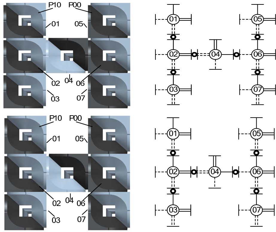
The dynamic address allocation process for a quadruped configuration

3.4 Functional Role Recognition for the Modules in the Configuration

An adjacency matrix is used to describe the connection relationship between the modules in the configuration. For the configuration of N modules, the adjacency matrix should be of dimensions N by N. To judge whether the topology adjacency matrix and the role connection matrix are isomorphic, we use a Nauty algorithm-based approach [28]. This is similar to the automatic matching for the configuration with fixed module IDs under the centralized control method, except for the dynamic module ID allocation process. Thus, we only describe the progress to identify the role of each module by comparing the local topology matrix.

Since the local topology matrix RS_Matrix can be divided into two parts - the adjacency matrix (ARS) and the connection orientation matrix (PRS) - the local topology configuration can be further expressed as follows: TC=(DV, ARS, PRS), where DV represents the assigned dynamic address vector during the stimulus signal transmission. First, the ARS of the shoulder module is fed into the Nauty program to obtain the module address mapping and the standard expression for the adjacency matrix. Second, the result is compared with the standard expression in the role modules' local topology library. If a match is found, then the connection orientation matrix is compared and the joint motion mapping relationship is subsequently generated. The functional role recognition process for the modules in the configuration is shown in Figure 6.

Figure 6.

Flow chart for the modules' functional role recognition

There are four different connection orientations {00 01 10 11} between any two modules. From the perspective of joint motion, orientation {00} and {10}, which can produce the same kind of joint motion, are called ‘Parallel Orientation’ and they are denoted by ; {01} and {11}, which can produce the same kind of joint motion, are called ‘Interleaved Orientation’ and they are denoted by . The red modules represent the role of the modules required to be identified.

3.5 Typical Configuration Identification and Adaptive Locomotion Generation

During the configuration-type identification, if the signal returned to the stimulus signal-generation module includes the roles of Spine, Shoulder, Knee and Foot, then the configuration can be determined as a quadruped-type; if the role is just Spine, then it is a chain-type.

When the stimulus signal for the configuration motion is finally sent, every module will receive the signal and execute the corresponding motions according to its own information as to the role, the connection orientation and the state flag; meanwhile, the signal will spread to other modules in the network through an effective connection.

From the module's role recognition process to the coordinated locomotion generation process, although the signal is sent out from the same module, the stimulus signal-generation module is not specified (i.e., any module can be assigned as the stimulus signal-generation module, which reflects the distributed nature of the algorithm).

The stimulus signal for the adaptive locomotion of the configuration will monitor the local topology, since each module initializes to execute any locomotion. Once the topology state array T_status [4] changes, the termination signal E0=[Halt; NUTT, C_Array] will be commanded and sent back to the stimulus signal-generation module along the path recorded in C_Array to stop the source module from generating the stimulus signal. Next, E1, E2, E3, E4…… will be resent from the source module. This shows that the algorithm can adapt to the dynamic changes in the network: when the configuration changes, the stimulus signal will re-identify the topology relationship, assign module ID dynamically, recognize the role of module, and ultimately generate the locomotion compatible with the configuration.

To prove the effectiveness of the distributed control algorithm, we take a worm configuration and a quadruped configuration as examples to describe the implementation process for configuration adaptability under this algorithm.

1. Worm Configuration

The worm configuration of six modules and its typical gaits are illustrated in Figure 7. Referring to the local topology table, the topological form can be clearly seen from left to right in the sequence: Role1_1, Role2_1, Role2_1, Role2_1, Role2_1 and Role1_1.

Figure 7.

The worm configuration of six modules and its typical gaits.

The simultaneous actuation of the corresponding component modules' joints to the appropriate angular position can result in crawling locomotion.

To accomplish squirming or other types of movement, traditional gait planning methods often require working out a locomotion control table oriented to a specific configuration, as shown in Table 2. In such a table, it is necessary to specify clearly the angular positions for each joint under each locomotion gait: each column represents a series of angular positions that a certain joint needs to reach in a cycle; each row represents the angular positions that all the modules in the entire configuration need to achieve under a certain gait. Under centralized control, the host computer needs to send the joint motion commands to all the modules in turn under each gait; after each joint has reached the required angular position, the host computer continues to send the next set of commands for the next gait, and so on, until the last gait of the cycle finishes; afterwards, another new but identical cycle will be repeated. AP represents the magnitude values of the joint angle, which will affect the volatility of the motion. The sign indicates the direction of rotation as either clockwise or counterclockwise.

Table 1.

Module local topology table

Table 2.

Motion control table for the worm configuration of six modules

Module Gait	M1	M2	M3	M4	M5	M6
1	+AP	-AP	-AP	+AP	+AP	-AP
2	-AP	-AP	+AP	+AP	-AP	-AP
3	-AP	+AP	+AP	-AP	-AP	+AP
4	+AP	+AP	-AP	-AP	+AP	+AP

For the motion control table under centralized control, many defects might emerge: whenever the configuration changes (e.g., when the local connection relationship alters) or the number of the modules differs, the table will need to be planned again as it is unable to adapt to the dynamic changes in the connection network; moreover, since every module needs to identify the commands according to its own ID, the host computer has to send the commands in turn, such that N² commands should be sent out in a configuration of N modules for N individual commands. The entire configuration locomotion will become more difficult to coordinate when the number of modules increases.

Specific to the worm configuration, a locomotion law can be easily found whereby the motion of each joint and the whole configuration observes the cycle style: each module has the same motion characteristic but only a phase difference between on another. For instance, the motion of module N at gait T is the same with module N- 1 at gait T+1. Thus, if a module selects a motion gait, the next module in the connection could choose its corresponding gait through local information to achieve coordinated locomotion. The transmission of the content-dependent stimulus signal proposed in our algorithm can accomplish such tasks. The content-based coordinated control rules are demonstrated in Table 3.

Table 3.

The content-based coordinated control rules for the worm configuration

Local Topology	Role Identification	Clock	Received Message	Action	Stimulus Signal
Role1_1	Head/Tail	0		AP	WE A R_direction
Role1_1	Head/Tail	T/4		-AP	WE B R_direction
Role1_1	Head/Tail	2T/4		-AP	WE C R_direction
Role1_1	Head/Tail	3T/4		AP	WE D R_direction
Role2_1	Spine		A	-AP	WE B R_direction
Role2_1	Spine		B	-AP	WE C R_direction
Role2_1	Spine		C	AP	WE D R_direction
Role2_1	Spine		D	AP	WE A R_direction

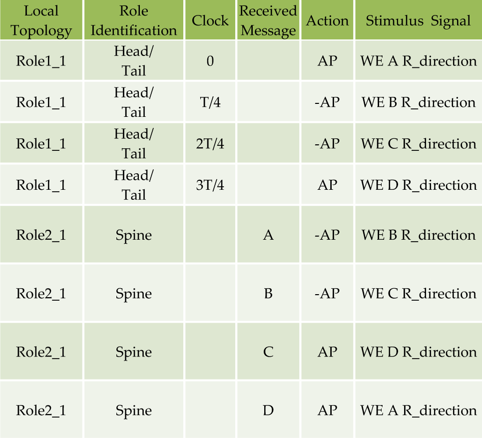
In this table, the complete movement period of the head module is set as T and the head module has to execute four gaits: AP, -AP, -AP and AP in a periodic cycle, so each gait consumes the time interval of T/4. We set the first module on the right terminal as the stimulus signal-generation module, which will continuously send the stimulus signal to generate the coordinated locomotion for the worm configuration after the module role recognition. The stimulus signal includes not only the feature symbol WE but also the control variables A, B, C, D and R_direction, which controls the transmission direction. ABCD in the fourth column represent the angular positions of the corresponding joint for the gait; the transmission direction control variable R_direction signifies that the stimulus signal that will be sent along the left or right direction to the module in the effective connection. When the next module receives the stimulus signal, it will map the motion to the corresponding joint according to the received stimulus signal, its local topology and the local connection information; meanwhile, it will update the stimulus signal and transmit it to the next module in the direction specified in the R_direction. When the stimulus signal is transmitted to the end of the configuration, it will stop spreading since there will be no more effective connection along the other directions. The velocity of the whole configuration is affected by the value of T: the smaller the value of T, the faster the configuration moves. However, T cannot decrease indefinitely because of hardware limitations.

2. Quadruped configuration

The quadruped configuration of 15 modules is shown in Figure 3. Similar to the worm configuration, the coordinated control rules are formulated as depicted in Table 4 to govern the stimulus signal transmission in order to achieve adaptive locomotion.

Table 4.

The coordinated control rules for the quadruped configuration

Local Topology	Role Identification	Clock	Received Message	Action	Stimulus Signal
Role3_5Role4_2Role4_4	Spine	0	Ch_D	Hold	LEDirection[RML-APB]Ch_D
Role3_5Role4_2Role4_4	Spine	T/2	Ch_D	Hold	LEDirection [RML-BPA]Ch_D
Role2_3	Shoulder		A	Swing Forward	LE A
Role2_3	Shoulder		B	Initial State	LE B
Role2_2	Knee		A	Lift and fall	LE A
Role2_2	Knee		B	Initial State	LE B
Role1_1	Foot		A	Cyclic_rotation	Null
Role1_1	Foot		B	Initial State	Null
Role2_1	Spine			Hold	Keep

The first three stimulus signals can accomplish such tasks as local topology information collection, functional role recognition and configuration identification. When the configuration is identified as the quadruped configuration, the regulation of the stimulus signal can lead to locomotion compatible with the quadruped configuration. In this table: for the spine module, ‘Hold’ means keeping the initial position of the module joint constant; for the shoulder module, ‘Swing forward’ represents the shoulder joint's swinging forward; for the knee module, ‘Lift and fall’ means the knee joint's swinging up and down upon completion of a leg-raising action; and for the foot module, ‘Cyclic rotation’ means the periodic rotary motion of the foot joint in assisting the completion of the leg's stepping movement; for all the modules, ‘Initial state’ means the initial joint posture of each module before any action. The stimulus signal includes the feature symbol LE, the signal transmission direction control variable Direction [RML-APB] and the transmission direction changing variable Ch_D. Assuming that Role3_5 is the source module, the stimulus signal is transmitted in the direction specified by Direction [RML-APB] (i.e., relative to the signal transmission direction), the right module delivers the stimulus signal {LE, A, null}, the left module conveys {LE, B, null}, the central module transmits {LE, Direction [RML-APB], Ch_D}, and the shoulder modules on both sides will complete the appropriate gaits according to the control variables A or B and will send the signal to the next module. The central signal is transmitted to Spine module Role3_5 through Spine module Role2_1. The signal will not change in Spine module Role2_1; however, when it reaches Spine module Role3_5, it will change the direction according to the direction symbol Ch_D (i.e., it will swap the left and right directions with the former Spine module Role3_5). The left module transmits the stimulus signal {LE, A, null} and the right module transmits {LE, B, null}; however, there is no signal transmission in the middle due to the absence of any effective connection. As a result of the existence of Ch_D, the modules in the diagonal direction move in the same manner in one gait, and they also observe intermittent motion when compared with the modules in the other diagonal direction. As such, coordinated locomotion can be realized for quadruped configuration.

The entire process is the transmission of one stimulus signal through the whole configuration. The Spine module Role3_5 will send the next stimulus signal after T/2, and the signal is pulsed and delivered at just such a frequency. Since the action execution time is much longer than the stimulus signal's transmission time, all the module joints are coordinated and almost move synchronously under the mechanism of distributed control.

4. Experimental Verification

4.1 Simulation for the Coordinated Motion of Typical Configurations under Distributed Control

The simulation environment is established in SPL for the coordinated locomotion of MSRR, where the basic physical properties of the module can be easily added to. The virtual environment supports the dynamics effects (e.g., collision, friction and so on), whereby the actual experimental situation can be simulated accurately. We construct the controller for each module, and the coordinated configuration motion can be realized by simulating the signal transmission mechanism of the distributed algorithm. The GUI of the simulator is shown in Figure 8.

Figure 8.

The GUI of the Simulator.

Oriented to the algorithm mentioned above, the two typical configurations - worm configuration and quadruped configuration - are constructed and tested. The results are shown in Figure 9.

Figure 9.

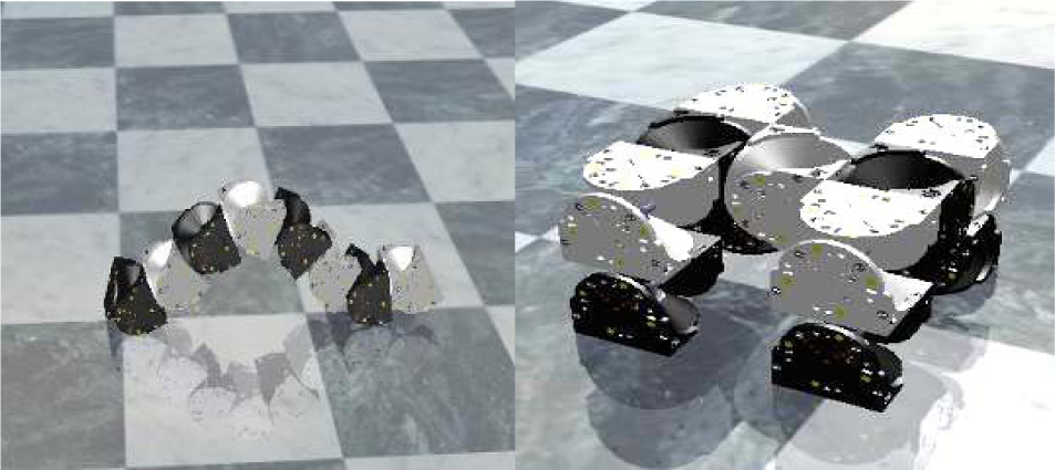
Simulation results in SPL.

4.2 Physical Experiments for the Coordinated Locomotion under Distributed Control

To verify the validity of the algorithm, we carried out experiments on the UBot MSRR robotic system on a flat table. The dimensions of a module are 80×80×80 mm. The mass of an active and a passive module is 350 g and 280 g, respectively.

Figure 10 shows the nine-module worm configuration experiment. The docking orientation between any module is {00} (i.e., a parallel orientation). Modelled on the transmission of water waves, each module generates a sinusoidal motion in turn to achieve the forward movement of the robot. The period of the sinusoidal motion is one second and the phase difference between each module is π/4. The locomotion is stable and smooth for the whole process: the robot moves 600 mm in 12 s and the velocity of the robot is about 50 mm/s. When the robotic system is powered up, the configuration will detect the local topology, recognize the modules' roles, map the joint motion coordinated by the stimulus pulse signal and, finally, will result in final coordinated locomotion.

Figure 10.

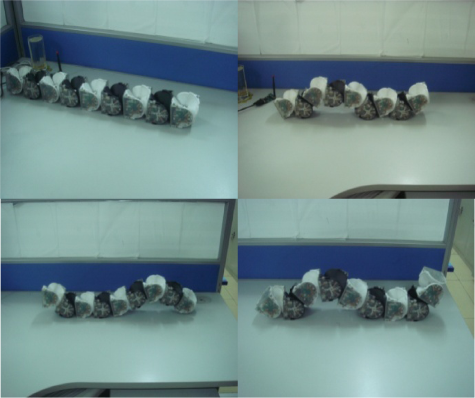
Coordinated locomotion of the worm configuration with nine modules.

In the same way, the quadruped motion experiment was completed on the UBot experimental platform. The docking orientation between the modules on the leg is {00}. As shown in Figure 11, the robot walks with the diagonal legs lifting and landing together. For the quadruped configuration, it is also a superposition of a series of sinusoidal motions. The speed of the joint is 120 degrees per second. The quadruped configuration walks forward at about 500 mm in 15 s, the velocity is about 33.3 mm/s. The result demonstrates that the locomotion is also stable and smooth, as expected.

Figure 11.

Coordinated locomotion for the quadrupedal configuration of 15 modules

The experiments fully prove the distributed feature of the algorithm, the dynamic adaptability to the connection topology changes, and the scalability in the number of modules. It validates the effectiveness of the stimulus pulse signal-based coordinated control algorithm for distributed locomotion.

5. Conclusion

This paper has presented a new approach for controlling MSRRs' coordinated locomotion using a stimulus pulse signal-based algorithm, which is distributed, adaptive and dynamic. Besides, it's also self-reconfigurable and has scalability to larger and multiple robotic systems. This approach enables configurations with certain typical configuration features to generate suitable locomotion gaits automatically. Experiments in terms of the worm configuration and the quadrupedal configuration in both actual Ubot modules and in 3D simulation have shown that this stimulus pulse signal-based distributed control algorithm can support many unique features of self-reconfigurable robots, which proves the validity of this algorithm.

Footnotes

6. Acknowledgments

The work reported in this paper is supported by the National Natural Science Foundation of China (Grant No. 60273316).

References

Liu

Zhu

Cui

Wang

Yan

Zhao

(2012) Multisensor-based autonomous docking for UBot modular reconfigurable robot. Proceedings of IEEE International Conference on Mechatronics and Automation (ICMA). 2012 Aug 5–8; Chengdu, China, pp. 772–776.

Shen

W. M.

Salemi

Will

(2002) Hormone-inspired adaptive communication and distributed control for CONRO self-reconfigurable robots. Robotics and Automation. 18(5): 700–712.

Yoshida

Murata

Kokaji

Kamimura

Tomita

Kurokawa

(2002). Get back in shape! [SMA self-reconfigurable microrobots]. Robotics and Automation. 9(4): 54–60.

Kotay

Rus

Vona

McGray

(1998). The self-reconfiguring robotic molecule. Proceedings of IEEE International Conference on Robotics and Automation (ICRA). 1998 May 16–20; Leuven, Belgium. pp. 424–431.

Ünsal

Kiliççöte

Khosla

P. K.

(2001). A modular self-reconfigurable bipartite robotic system: Implementation and motion planning. Autonomous Robots. 10(1): 23–40.

Suh

J. W.

Homans

S. B.

Yim

(2002). Telecubes: Mechanical design of a module for self-reconfigurable robotics. Proceedings of IEEE International Conference on Robotics and Automation (ICRA). 2002 May 11–15; Washington, DC, USA. pp. 4095–4101.

Bordignon

Stoy

Schultz

U. P.

(2009). A virtual machine-based approach for fast and flexible reprogramming of modular robots. Proceedings of IEEE International Conference on Robotics and Automation (ICRA). 2009 May 12–17; Kobe, Japan. pp. 4273–4280.

Zykov

Mytilinaios

Adams

Lipson

(2005). Self-reproducing machines. Nature. 435(7038): 163–164.

Sproewitz

Billard

Dillenbourg

Ijspeert

A. J.

(2009). Roombots-mechanical design of self-reconfiguring modular robots for adaptive furniture. Proceedings of IEEE International Conference on Robotics and Automation (ICRA). 2009 May 12–17; Kobe, Japan, pp. 4259–4264.

10.

Yim

Roufas

Duff

Zhang

Eldershaw

Homans

(2003). Modular reconfigurable robots in space applications. Autonomous Robots. 14(2–3): 225–237.

11.

Yim

Shirmohammadi

Benelli

(2007). Amphibious modular robotic astrobiology. Proc. of SPIE. 2007 Nov 15–17; Wuhan, China, pp. 65611S–1.

12.

Stoy

Brandt

Christensen

D. J.

(2010). An Introduction to Self-Reconfigurable Robots. Massachusetts: MIT Press. pp. 27–32.

13.

Gilpin

Rus

(2010). Modular robot systems. Robotics and Automation. 17(3): 38–55.

14.

Murata

Kurokawa

(2012). Self-organizing robots. Verlag: Springer, pp. 110–114.

15.

Fukuda

Nakagawa

(1988). Approach to the dynamically reconfigurable robotic system. Journal of Intelligent and Robotic Systems. 1(1): 55–72.

16.

Kurokawa

Tomita

Kamimura

Kokaji

Hasuo

Murata

(2008). Distributed self-reconfiguration of M-TRAN III modular robotic system. The International Journal of Robotics Research. 27(3–4): 373–386.

17.

Shen

W. M.

Krivokon

Chiu

Everist

Rubenstein

Venkatesh

(2006). Multimode locomotion via SuperBot reconfigurable robots. Autonomous Robots. 20(2): 165–177.

18.

Sprowitz

Pouya

Bonardi

Van den Kieboom

Mockel

Billard

Ijspeert

A. J.

(2010). Roombots: reconfigurable robots for adaptive furniture. Computational Intelligence Magazine. 5(3): 20–32.

19.

Østergaard

E. H.

Kassow

Beck

Lund

H. H.

(2006). Design of the ATRON lattice-based self-reconfigurable robot. Autonomous Robots. 21(2): 165–183.

20.

Kernbach

Meister

Scholz

Humza

Liedke

Ricotti

Liu

(2009). Evolutionary robotics: the next-generation-platform for on-line and on-board artificial evolution. IEEE Congress on Evolutionary Computation, 2009 May 18–21; Trondheim, Norway. pp. 1079–1086.

21.

Wei

Chen

Tan

Wang

(2011). Sambot: A self-assembly modular robot system. Mechatronics. 16(4): 745–757.

22.

Zhao

Cui

Zhu

Tang

(2011). A new self-reconfigurable modular robotic system UBot: Multi-mode locomotion and self-reconfiguration. Proceedings of IEEE International Conference on Robotics and Automation (ICRA). 2011 May 9–13; Shanghai, China. pp. 1020–1025.

23.

Meng

Zhang

Sampath

Jin

Sendhoff

(2011, May). Cross-ball: a new morphogenetic self-reconfigurable modular robot. Proceedings of IEEE International Conference on Robotics and Automation (ICRA). 2011 May 9–13; Shanghai, China, pp. 267–272.

24.

Davey

Kwok

Yim

(2012). Emulating self-reconfigurable robots-design of the SMORES system. International Conference on Intelligent Robots and Systems (IROS). 2012 Oct 8–11; Algarve, Portugal. pp. 4464–4469.

25.

Tang

Zhu

Zhao

Cui

(2009). The UBot modules for self-reconfigurable robot. International Conference on Reconfigurable Mechanisms and Robots (ReMAR). 2009 Jun 22–24; London, England, pp. 529–535.

26.

Zhao

Tang

Zhu

Cui

(2010). A Modular Self-reconfigurable Robot Based on Universal Joint. Robot, 32(5): 6.

27.

Zhao

Tang

S. F.

Zhu

Y. H.

Cui

X. D.

(2011). Topological description method of UBot self-reconfigurable robot. Journal of Harbin Institute of Technology. 43(1): 46–49, 55.

28.

Tang

(2010). Research of self-reconfigurable robot based on universal joint module [PhD thesis]. Harbin: Harbin Institute of Technology.

Module Gait	M1	M2	M3	M4	M5	M6
1	+AP	-AP	-AP	+AP	+AP	-AP
2	-AP	-AP	+AP	+AP	-AP	-AP
3	-AP	+AP	+AP	-AP	-AP	+AP
4	+AP	+AP	-AP	-AP	+AP	+AP

Module Gait	M1	M2	M3	M4	M5	M6
1	+AP	-AP	-AP	+AP	+AP	-AP
2	-AP	-AP	+AP	+AP	-AP	-AP
3	-AP	+AP	+AP	-AP	-AP	+AP
4	+AP	+AP	-AP	-AP	+AP	+AP

Stimulus Pulse-Based Distributed Control for the Locomotion of a UBot Modular Robot

Abstract

Keywords

1. Introduction

2. UBot MSRR System

2.1 UBOT Module

2.2 Local Communication Interface for Distributed Control

3. The Stimulus Pulse Signal-based Distributed Control Algorithm for Coordinated Locomotion

3.1 Topological Formulation of Ubot MSRR's Configuration

3.2 Stimulus Pulse-based Distributed Control for Coordinated Locomotion

3.3 Dynamic Address Allocation for the Modules in the Network

3.4 Functional Role Recognition for the Modules in the Configuration

3.5 Typical Configuration Identification and Adaptive Locomotion Generation

4. Experimental Verification

4.1 Simulation for the Coordinated Motion of Typical Configurations under Distributed Control

4.2 Physical Experiments for the Coordinated Locomotion under Distributed Control

5. Conclusion

Footnotes

6. Acknowledgments

References

Module Gait	M1	M2	M3	M4	M5	M6
1	+AP	-AP	-AP	+AP	+AP	-AP
2	-AP	-AP	+AP	+AP	-AP	-AP
3	-AP	+AP	+AP	-AP	-AP	+AP
4	+AP	+AP	-AP	-AP	+AP	+AP