Sage Journals: Discover world-class research

Abstract

In this paper, we address the problem of mapping outdoor rough terrain environments for mobile robots. While uncertainties arising from multiple sources are considered explicitly and assumed to be unknown-but-bounded, a set-theoretic framework is proposed to construct the terrain model as a set-valued elevation map that extends the notion of the elevation map with elevation variation in each cell stored by intervals. The localization problem of the mobile robot is also considered and solved by a set-membership filter in order to provide guaranteed bounded-pose estimation, which can be incorporated to the elevation map to improve the accuracy of the final terrain model. A more compact terrain representation can be obtained by the proposed algorithm with relatively low computational complexity, which makes it suitable for real-time applications. Furthermore, improved smoothness is achieved by the inherent conservativeness of the set-theoretic method without additional filtering or interpolation processes. Simulations as well as real-life experiments of a mobile robot operating in outdoor rough terrain environments with a 2D scanning laser rangefinder demonstrate the effectiveness and robustness of the proposed method.

Keywords

Mobile Robot Terrain Estimation Elevation Map Set-Valued Bounded Error

1. Introduction

With the expansion of mobile robot applications, such as planetary and polar exploration, seafloor studies, urban reconnaissance and rescue mission scenarios, etc., research into field robotics for outdoor environments is receiving increasing attention [1 –4]. Among these applications, autonomous 3D environment modelling (or ‘mapping’) is a primary and crucial problem, as it can provide necessary environmental representations for the accomplishment of successful outdoor tasks, including self-localization, path planning, obstacle avoidance and object detection, etc. Compared to the 2D mapping of indoor environments, the 3D modelling of outdoor environments appears to be more challenging, because such environments are highly diverse, unstructured or even dynamic, all of which make it difficult to construct uniform models of these environments. Another problem that should be taken into account is the trade-off between the richness of terrain presentation and computational complexity.

In recent years 3D mapping has attracted substantial interest in the robotics community. Papadakis [5] has recently made a comprehensive survey of the state-of-the-art of terrain mapping and traversability analysis technologies. The simplest and most widely used approach is the voxel-based algorithm, which divides the robot environment into voxels with 3D geometric data. Some pioneering works have been done by Elfes [6] and Moravec [7], in which the 2D occupancy grid method is extended to a 3D occupancy grid to represent the environment with stereo vision sensing. Furthermore Tirumalai et al. [8] and Pagac et al. [9] employ 3D grid representation to model the environments in their experiments using the Dempster-Shafer theory for evidential reasoning and the fusion-of-depth information that comes from stereo vision and sonar, respectively. Roth and Wibowoo [10] propose a volumetric method that can create triangular meshes by translating point data from a laser scanner. Thrun et al. [11] use a fine-grained textured polygon surface model to obtain a more compact representation of environments with a laser rangefinder (LRF). Other recent advances include an octree-based 3D environment description that compresses and stores voxels in an octree structure or else use multi-resolution voxels [12, 13]. Though all these voxel-based geometric methods can produce rich and dense maps, they are often constrained to indoor or structured environments. Moreover, they are not suitable for real-time applications because of the high computational complexity required to maintain and update the created map, especially in the case of large-scale environments.

An attractive alternative mapping technique would be to construct an elevation map, which has been introduced as a more compact 2.5D representation of outdoor unstructured environments. The key idea underlying an elevation map is to represent environments with 2D grids, with a dominant height value of the corresponding terrain stored for each grid. This kind of map can capture the richness of environmental information with a lower computational burden than the voxel-based map. Hoffman and Krotkov [14] build an elevation map of terrain using a LRF mounted on a legged robot, and the perceived maximum height is assigned to the terrain. Hygounenc et al. [15] work on the construction of a digital elevation map by tracking and matching landmarks with a blimp robot using low altitude stereovision. Ye and Borenstein [16] propose an algorithm to acquire elevation maps with a 2D LRF, and a novel filter is used to eliminate measurement errors or other noise. Miller and Campbell [17] propose a real-time mixture-model-based algorithm by using Gaussian sum elevation density to model terrain variation in an elevation map. With their method, the uncertainties from different sources are considered for the first time and modelled as Gaussian distributions. Kleiner and Dornhege [18] introduce a similar Gaussian distribution-based terrain estimation method for building an elevation map by utilizing EKF to integrate range measurements from a downwards-tilted LRF. All of the above elevation map-based approaches lack the ability to represent vertical structures or even multiple levels of terrain. Pfaff et al. [19] extend an elevation map to deal with vertical and overhanging objects by a classification approach. Revadeneyra et al. [20] propose a multi-level surface map to store multiple surfaces in each cell of the grid with Gaussian fusion. In these studies, uncertainties from different sources are not considered explicitly. Vasudevan et al. [2, 21] use the non-stationary (neural network) Gaussian process to model large-scale terrains in order to handle the uncertainty and incompleteness of sensory information, which can provide a multi-resolution representation of space to ensure local smoothness while preserving the characteristic features of rich and complex terrain data. In our previous work [22], the set-membership idea is first introduced to terrain mapping, in which the errors of point clouds are assumed to be unknown-but-bounded (UBB) noises so that they can be compensated to the terrain model. However, the details of this new terrain modelling algorithm are rather rough. Only a simple simulation analysis and a few experimental results are given in the paper.

Other 3D mapping techniques include constructing Monte Carlo-sampled environments [23], creating point cloud maps [24], and presenting sensor data using true 3D terrain maps [25]. These approaches either suffer from high computational complexity or else are constrained to structured environments.

In this paper, the idea of using a uniform set-theoretic framework for outdoor terrain mapping proposed in our previous work [22] is extended and discussed in detail. Uncertainties from different sources are assumed to be UBB errors. No other prior knowledge is needed here. Depth measurements obtained by a scanning LRF are first transformed to bounded elevation estimations of corresponding terrains as global Cartesian coordinates. Next, every estimated elevation is assigned to one or more grid cells that it is likely to belong to by detecting its uncertainty bounds. Finally, all the bounded elevations that are associated with the same cell are fused to produce the set-valued estimation of the terrain in that cell. To be consist with the set-theoretic framework, an extended set-membership filter [26] is used here to solve the localization problem and provide the bounded pose estimation of the mobile robot, which can be fused to the current elevation map so as to improve the accuracy of the terrain model.

The proposed approach contains contributions at different levels. First, uncertainties are considered explicitly and assumed to be UBB errors in the set-theoretic (also called ‘set-valued’ or ‘set-membership’) framework. This assumption provides an interesting alternative for traditional stochastic assumptions in which the known probabilistic distribution (such as the widely-used Gaussian distribution) of errors should be given. In many cases, it seems to be more practical than the stochastic methods, because bounds of errors can be more easily obtained or validated than probabilistic distributions. Second, the proposed set-valued elevation map extends the traditional elevation map to provide an elevation variation estimation for each cell. The guaranteed bounded terrain estimation is produced so that more detail and richness in the terrain model are introduced - for example, the roughness of the terrain in each cell can be initially determined. The robustness of the whole algorithm can be improved accordingly because of the conservativeness inherent in the set-membership theory [26] - that is, the rigorous hard bounds of the elevation variance for each cell in which the real elevations are guaranteed to fall in are obtained with bounded error assumptions. This profit could be very important for successive path planning and pose reconfiguration problems, especially for field robots with highly stability and reliability requirements. Third, because the interval description of a feasible set is adopted in our paper to apply the set-membership framework, our method provides a simple but computationally-efficient algorithm to store and update the full terrain model with limited time and space complexity, which makes it suitable for online applications. In addition, our proposed algorithm can output a smoother terrain estimation, and a potential filtering effect is achieved by the inherent conservativeness of the set-valued framework. Finally, the localization problem of the robot is also solved by a set-membership filter. The fusion between terrain and pose information can be performed in a natural manner to further improve the detail of the created environment model.

2. Problem formulation

In our algorithm, a set-theoretic framework based on set-valued representation and estimation is adopted instead of probabilistic approaches in order to construct a terrain estimation algorithm. In this framework, all uncertainties or disturbances are assumed to be UBB errors with known magnitudes of bounds. Upon this UBB assumption, state-bounding techniques - such as interval analysis [27] or a set-membership filter [28] - can be used to propagate the uncertainties through transformations, so as to provide guaranteed bounded estimations of states, which can be treated as physical constraints in successive planning and decision procedures.

Definition 1 (Feasible set): Given a nonlinear function y = f( x ), where f : ℝⁿ → ℝ^m is a real function and x ∊ X ℝⁿ represents the variable with determined bounds, the feasible set of y can be denoted as the following set-valued function:

Y = f (X) = {f (x) | x \in X} \subseteq ℝ^{m}

(1)

The exact representation of a feasible set is often hard to calculate, which makes the computation load of the algorithm prohibitively high for real-time applications. In view of this, regular geometry shapes that out-bound the feasible set, such as intervals, ellipsoids, parallelotopes and zonotopes, are used to approximate the feasible set to reduce computational complexity. In this paper, the interval-based description of a feasible set is adopted because of its lower demands for information in representing the feasible set and its simpler manner of bounding which make it convenient for the uncertainty descriptions and state bounding.

Definition 2 (Interval): An n-dimensional interval (namely an axis-aligned box) I_x can be defined as a closed, connected and bounded subset of ℝⁿ, that is:

ℐ ​_{x} = [x] = [\underline{x}, \bar{x}] = {x \in ℝ^{n} : {\underline{x}}_{i} \leq x_{i} \leq {\bar{x}}_{i}, i = 1, 2, …, n}

(2)

where $\bar{x} = {({\bar{x}}_{1}, {\bar{x}}_{2}, …, {\bar{x}}_{n})}^{T} \in ℝ^{n}$ is the upper bound and $\underline{x} = {({\underline{x}}_{1}, {\underline{x}}_{2}, …, {\underline{x}}_{n})}^{T} \in ℝ^{n}$ is the lower bound of I_x, respectively. An alternative equivalent expression of the interval can be given as:

I ​_{x} = [\hat{x} - δ_{x}, \hat{x} + δ_{x}]

(3)

where ○ and δ_x are the centre (mid-point) and radius of I_x respectively:

\hat{x} = (\underline{x} + \bar{x}) / 2, δ_{x} = (\bar{x} - \underline{x}) / 2

(4)

Arithmetical operations used for real numbers can easily be extended for intervals, as with the following definition.

Definition 3 (Interval arithmetic): The arithmetic of an interval is defined as:

[x_{1}] \circ [x_{2}] = {x_{1} \circ x_{2} | x_{1} \in [x_{1}], x_{2} \in [x_{2}]}, \forall \circ \in {+, -, *, /}

(5)

Other mathematical operations such as trigonometric functions and exponential functions can be defined similarly. Generally, a real function of an interval variable is defined as follows.

Definition 4 (Inclusion function): Let f: ℝⁿ → ℝ^m be a real function, such that the feasible set of this function over an interval variable [x] is given by:

f ([x]) = {f (x) \in ℝ^{m} | x \in [x], [x] \subseteq ℝ^{n}}

(6)

The shape of f ([ x ]) is often complex and is not even necessarily an interval under nonlinear functions. The solution is to use an outer bounding interval to approximate the feasible set. Moreover, as the point-wise computation of (6) will entail huge computational loads, a better approach is to find an inclusion function [ f ] for f that satisfies:

f ([x]) \subseteq [f] ([x])

(7)

which will give an outer bounding interval of the true feasible set for a continuous function f with reduced computational loads. It should be noted that the selection of an inclusion function is not unique. Care has to be taken to correctly implement the inclusion function, such that the conservatism is minimized when evaluated. For example, for the function y = f (x) = x², x ∊[–1,1], if we choose an inclusion function[f]([x]) = [x][x], the result is [y] = [–1,1]; alternatively, if we choose another inclusion function [f] ([x]) = [x]², the result is [y] = [0,1], which gives the true value of f([x]). More details about interval analysis can be found in [27] and [29]. The existence and convergence of an inclusion function are given as the following Lemma [29]:

Lemma 1: Consider the function: f : ℝⁿ → ℝ, where (x₁,…,x_n) → (f(x₁,…,x_n)) is expressed as a finite composition of the operators +, -, * and / and elementary functions (sin, cos, etc.). An inclusion monotonic and thin inclusion function [f] : ℝ_n → ℝ for f is obtained by replacing each real variable x_i with the interval variable [x_i], and each operator and function by its interval counterpart. If f involves only continuous operators and functions, [f] is convergent. If each of the variables (x₁,…, x_n) occurs at most once in f, [f] is also minimal.

3. Set-theoretic terrain estimation

The set-theoretic terrain estimation algorithm proposed in this paper adopts a unified set-valued framework instead of the popular probabilistic methods mentioned above. The key idea of this algorithm is to represent uncertainties and elevation values with bounded sets, like intervals. In view of the interval description, interval analysis theory can be used to transform and fuse the sensor data in a natural manner so as to construct a so-called set-valued elevation map in which the terrain variation for each cell is taken into account. The whole algorithm can be divided into three steps: the first step is to construct the sensor model with UBB multi-source uncertainty assumptions and then transform depth measurements in local sensor coordinates to bounded elevation estimations in global Cartesian coordinates; the second step is to assign the elevation estimations obtained in the previous step to one or more cells by detecting their variation bounds; the last step is to update the elevation map by fusing the current estimated elevation intervals with the original estimations in associated cells. With these three steps, each sensor measurement is processed through an iterative process to contribute to the final terrain model. Compared to traditional probabilistic terrain modelling methods, this new deterministic set-theoretic terrain estimation algorithm may introduce more richness and robustness with limited computational complexity. Moreover, better smoothness will be achieved by the inherent conservativeness of the set-theoretic method and without any extra filtering or interpolation process.

3.1 Elevation modelling

In a traditional elevation map, the horizontal ground is divided into grid-cells of the same size, and a single height value is assigned to each grid cell to denote the dominant elevation within it. This 2.5D representation method is popular in outdoor applications because of its adaptability to different kinds of unstructured terrain. However, more attention should be given to the problem of maintaining the balance between the richness and computational complexity of the map. In order to capture more details of the terrain, grid cells of a smaller size should be used which, however, will increase the computational burden of the algorithm and make it impractical for real-time applications, especially for large-scale environments. In addition, too small a cell size will lead to no assignment of measurements for many cells, and extra interpolations will be needed to fill gaps in the map. Another drawback of the traditional elevation map is that only a dominant elevation is given for each cell, even when several measurements that are greatly different from each other may be associated to the same cell, resulting in an informational loss for those cells with multi-elevation features, such as vertical structures. Therefore, the traditional elevation map is unsuitable for capturing rapidly changing terrains or multi-elevation terrains.

In this paper, a novel extended elevation map is introduced to overcome the above mentioned drawbacks of traditional elevation maps, while still keeping a reasonable trade-off between model accuracy and computational burden. The elevation variation for each cell is taken into account and represented by a set-valued style, such as an interval. An elevation interval can provide a guaranteed range for the elevation variations of each cell with contemporaneous measurements. More details of the terrain in each cell - such as multi-elevation features or roughness - can be presented naturally through this set-valued elevation model, which seems to be more useful in the path planning and configuration adjustment tasks of field robots with high reliability and stability demands. An example of the set-valued elevation model is depicted in Figure 1.

Figure 1.

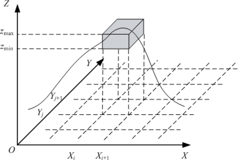
Set-valued elevation model for 3D terrain

The global Cartesian coordinates OXYZ are selected as follows: the origin O is selected as a random point of interest; the horizontal plane is defined as the XOY plane; and the OZ axis is finally chosen as being perpendicular to the XOY plane in order to construct a right-handed coordinate system. In outdoor environments, a widely-used global Cartesian coordinate system is the WGS-84 ellipsoid model of the Earth. The origin O is selected as a point of interest at this place. The horizontal plane is selected as the tangent plane of the ellipsoid at this origin, where the OX axis points east along the latitude, OY points north along the longitude, and OZ points up along the vertical. The 3D position of a terrain point can be described naturally by its east-north-up (ENU) coordination.

As indicated in Figure 1, the horizontal position of a sampled terrain feature is represented by the grid cell c_ij (i, j ∊ ℤ are integral indices) that it falls to, where c_ij denotes the cell composed by all points (x, y, z):

X_{i} \leq x < X_{i + 1}, Y_{j} \leq y < Y_{j + 1}

(8)

with:

X_{i} = s i, X_{i + 1} = s (i + 1), Y_{j} = s j, Y_{j + 1} = s (j + 1)

(9)

where s denotes the cell dimension, the terrain in the cell c_ij is denoted by an interval $ℐ _{i j} = [z_{\min}, z_{\max}]$ , and where z_min and z_max stand for the highest and lowest elevation values that may be contained in this cell.

3.2 Measurements modelling and transformation

In this step, the sensor model is constructed by explicitly taking multi-source uncertainties into account. Measurements will be transformed to elevation estimations in the global coordinates with the sensor model. In parallel, uncertainties will be propagated to enhance the robustness of the terrain estimation.

As discussed in previous works, uncertainties related to the sensor model occur for various reasons [17, 18]. In general, the main sources of error are induced by the following three causes:

Measurement errors due to hardware limits;

Calibration errors of sensors (that is, errors between the measured and true poses of sensing platforms);

Errors caused by the inaccurate pose estimation of the robot.

In this paper, uncertainties are assumed to be UBB errors in accordance with the set-valued framework. This deterministic assumption provides an attractive alternative when compared to stochastic assumptions with known probabilistic distributions (such as the Gaussian distribution assumption mentioned above). In many cases, the UBB assumption seems to be more practical in real-time applications, because to determine and verify bounds of errors seems much easier than probabilistic distributions. For example, the accuracy of a sensor is often given in the form of the bounded error of the current measurement, such as the LRF used in our paper. As for the calibration errors of sensors and the pose errors of the robot, it may also be easier to determine outer bounds than the distribution approximation of errors. In the worst case, an over-estimated bound can be used if not enough prior information can be obtained.

To transform measurements in a local sensor coordination frame to elevation values in the global Cartesian coordinates frame, the following transformation matrix T is created by q-level coordinates' transformations using left multiplications of the matrix:

T = T_{q} (p_{q}) T_{q - 1} (p_{q - 1}) \dots T_{1} (p_{1}) R (r)

(10)

where T_i( p _i ), i = 1, 2, …, q denotes the transformation matrix of the q-level sub-platforms from the sensor platform to the global coordinates, p _i are parameter vectors contained in T_i, with UBB uncertainties related to 2) and 3) defined above, R and T are the matrix representations of the raw measurements in the sensor coordinates and the elevation estimation in the global coordinates, respectively, and r is the raw measurement vector with UBB uncertainty defined in 1). The measurement model can be defined as:

x = f (p, r) = T (p_{1}, p_{2}, …, p_{q}, r)

(11)

where x = (x y z)^T is the transformed elevation value and p=(p₁^T,p₂^T,…,p_q^T )^T is the parameter vector comprising p _i , i = 1, 2, …, q defined in (10).

Considering the UBB noise assumption for r and p , the interval description is used here, such that:

I_{p} = [p] = [\hat{p} - δ_{p}, \hat{p} + δ_{p}], I_{r} = [r] = [\hat{r} - δ_{r}, \hat{r} + δ_{r}]

(12)

where p̂ is the reference parameter vector, r̂ is the raw measurement vector, and δ_p and δ_r are uncertainty radii. The set-valued elevation estimation can be given as:

f ([p], [r]) = {f (p, r) | p \in [p], r \in [r]}

(13)

For most real-life robotic applications where f is a continuous function related to p and r , an outer bounding interval description of a feasible set can be obtained by using an inclusion function [ f ]:

I_{x} = {([x], [y], [z])}^{T} = [f] ([p], [r]) \supseteq f ([p], [r])

(14)

Otherwise, an outer bounding interval of [ f ] ([ p ], [ r ]) should be selected for I_x.

3.3 Elevation assignment

After transforming a raw measurement into an elevation estimation in global coordinates, the next step is to assign this set-valued elevation estimation to the cells that it is likely to belong to. During the above transformation step, uncertainties are propagated into the obtained elevation interval, which results in a guaranteed bounded elevation estimation with the true terrain height lying in the terrain interval. Due to the set-valued description, the estimated elevation will not be assigned to just a single cell but rather to several cells in a local area S determined by the bounds of the elevation interval, that is:

S = [x] \times [y] = {(x, y) \in^{} ℝ^{2} | x \in [x], y \in [y]}

(15)

where the intervals [x] and [y] are obtained by (14). These two intervals can be rewritten as:

[x] = [\underline{x}, \bar{x}], [y] = [\underline{y}, \bar{y}]

(16)

The cell indices i₁, i₂, j₁ and j₂ are selected to satisfy:

s X_{i_{1}} \leq \underline{x} < s X_{i_{1} + 1}, s X_{i_{2}} \leq \bar{x} < s X_{i_{2} + 1}

(17)

s Y_{j_{1}} \leq \underline{y} < s Y_{j_{1} + 1}, s Y_{j_{2}} \leq \bar{y} < s Y_{j_{2} + 1}

(18)

The set of cells that the current elevation interval should be assigned to can be defined as follows:

{(X_{i}, Y_{j}) | i, j \in ℤ, i_{1} \leq i \leq i_{2}, j_{1} \leq j \leq j_{2}}

(19)

3.4 Elevation fusion and map updating

The last step is to fuse the current elevation estimation into the associated cells defined by (19) so as to update the elevation map. This procedure is only carried out in a local area of the map in order to reduce the computational burden of the algorithm. For each cell (X_i, Y_j) defined in (19), given the current estimated elevation interval [z_i,j]^cur and the new assigned elevation interval [z] obtained by (14), the fusion process can be achieved in a natural manner, that is, by the union operator of these two intervals:

I_{i, j}^{new} = {[z_{i, j}]}^{new} = {[z_{i, j}]}^{cur} \cup [z]

(20)

It should be noted that the fusion is performed by the interval union operator instead of the intersection operator. The reason is given below: each measurement is obtained independently with different poses of the robot or view points of the sensor, and so the estimated elevations are always related to different terrain features whether they belong to the same cell or not. In fact, even if two measurements belong to the same cell, the corresponding true terrain points sensed by the robot are almost distinct from one other. That is to say, each estimated elevation from a new measurement may contain new terrain information for their associated cells, which can be used to improve the accuracy of the terrain model and provide more detail such as the roughness of the cells. The intersection operator would result in erroneous terrain estimations, with information loss and gaps for many cells. In contrast, the union operator can make use of all the associated measurements to record the terrain variation of cells, which makes it more suitable for elevation fusion.

3.5 Algorithm summary

The iterative updating steps of the set-valued terrain estimation algorithm are summarized in this section.

Given a new measurement vector r with a corresponding model parameter vector p , the terrain model will be updated as follows:

Step 1: Compute the set-valued elevation estimation I_x with r and p by (14);

Step 2: The set {(X_i, Y_i)} of cells (X_i, Y_i) that the set-valued elevation I_x should be assigned to is computed by (17)–(19);

Step 3: For each cell (X_i, Y_i), the elevation estimation is updated by (20).

Compared to probabilistic approaches, the set-theoretic terrain mapping algorithm can replace the stochastic assumptions of uncertainties by UBB errors, and are more practical and seem to be much easier to verify in many cases. The established set-valued elevation map extends the traditional elevation map by providing an elevation variation range for each cell. The guaranteed, bounded, rough terrain, environmental information can be obtained within this set-theoretic framework, which can be used as a physical constraint for planning and control tasks with a view to improving the robustness and reliability of the system. Moreover, as the UBB uncertainties are propagated to the estimated set-value elevation through the measurement model, the robustness of the algorithm is enhanced with increased conservativeness, which makes a measurement assigned to more than one cell in a local area and, therefore, contributes to the elevation model of all these cells. A potential terrain filtering is accomplished with the introduction of more smoothing into the final terrain model, while some gaps stemming from the absence or occlusion of measurements will be filled without any extra interpolation operation.

The terrain modelling algorithm proposed here is computationally efficient and suitable for real-time applications, even for large-scale outdoor environments. Regarding the space complexity, the interval elevation map only needs to store the estimated elevation interval of each grid cell, so the memory requirements of the algorithm are limited to O(N), where N is the number of cells in the whole map. As to time complexity, the algorithm is carried out iteratively. Moreover, instead of updating the entire map, only a local area of the map needs to be updated for each new measurement. With this locally-updating strategy, the time complexity of the algorithm is reduced from O(MN) to O(kM), where M is the number of measurement scans and k is the maximum number of the cells that a measurement may assigned to. Normally, we have k « M. The above analysis shows that the proposed new algorithm can maintain a good balance between the map's richness and computational complexity, which makes it possible to create, maintain and update the terrain map online for large-scale environments.

It should be noted that though the interval description is adopted here to denote the feasible set for the elevation estimation, other shapes such as ellipsoids and parallelotopes are also available to solve this problem. Similar derivations can be made within the uniform framework of set-theoretic approaches.

4. Set-membership-based localization

The application of the terrain estimation algorithms is based on two pre-conditions: the measurement r and the parameter p with the uncertainty bounds δ_r and δ_p;. The measurement r is acquired by a sensing device, with δ_r determined by the accuracy of the sensor used. The model parameter vector p can be classified into constant and variable components. Constant parameters, such as the calibration parameters of the sensor platform, can be determined by used calibration means. Varying parameters, mainly the pose of the mobile robot, can be solved by real-time localization approaches. Unlike the previous 2D localization studies implemented in indoor environments, the full 3D pose of the robot should be considered for outdoor terrain environments. Future studies will be performed to detect the loop closure, based on scan matching or other approaches, to simultaneously solve localization and terrain modelling problems, which lead to the so-called simultaneous localization and mapping (SLAM) problems [28].

The observation model of the robot should be created according to sensors that are used for the task of localization. An odometer can be used to give the displacement of two wheels, with GPS integrated to reduce the unbounded accumulative error brought by the odometer, especially in large-scale environments. An inertial measurement unit (IMU) or tilt sensors (accelerometers or gyroscopes) can give the orientation of the robot with bounded error. Other technologies include the visual odometer technique with a stereo camera.

To be compatible with the above-established set-theoretic environment mapping approaches, set-valued estimators such as the set-membership filter (SMF) should be used in tracking the pose of the mobile robot [30], which can provide a guaranteed, bounded pose estimation [ p _r] of the robot. Additional details of the SMF localization can be found in our previous work in [26].

In addition, the estimated set-valued pose of the robot by SMF contains the terrain information for the ground cells it travels across. More detail for those cells can be obtained by fusing the pose into the elevation model, which will improve the performance of the algorithm and produce a denser map. Under the set-valued framework, union operation is again used to fuse the elevation [z_r] from the pose estimation and the original elevation estimation [z] for each cell, as follows:

I^{new} = [z] \cup [z_{r}]

(24)

Note, again, that the union operator for intervals are used here as in (20), because the terrain information given by the pose estimation may not be observed by the robot, for example, due to coarse discretizations or occlusions. The union operator will incorporate the different terrain information from both the pose and elevation estimations so as to provide more accurate terrain variation estimations.

5. Simulations

In this section, the set-valued terrain estimation algorithm will be compared to the Gaussian mixture model (GMM) based on a real-time terrain estimation algorithm (adopted by Team Cornell for the Grand Challenge and other researchers) [17, 18] for 1D terrain environments. The robot platform is described in Figure 2.

Figure 2.

The simulated robot with a LRF

The velocity of the robot is set to v = 5 m/s. The localization error is set to δ_x = 0.6 m. A LRF is mounted on the vehicle with a pitch angle of φ = −5° (calibration error δ_φ = 0.5°) and a height of h_m = 1.5 m (no calibration error). The measurement from the LRF is denoted by r with an accuracy of δ_r = 0.1 m, and the sample frequency is assumed to be f = 75 Hz. The simulated 1D terrain is a hypothetical ground that can be divided into several segments: flat segments with different heights (flat terrain) in 0 m ≤ x < 40.5 m, 45.5 m ≤ x < 70.5 m, 70.5 m ≤ x < 100.5 m and 100.5 m ≤ x < 150.5 m; a plateau in 170.5 m ≤ x < 200 m with a vertical wall at x = 170.5 m; a small ditch in 150.5 m ≤ x < 155.5 m; a slope in 40.5 m ≤ x < 45.5 m as shown in Figure 3. Here, all the terrain changes are set to happen in cells instead of among the bounds between cells. The cell size of the elevation map is chosen as s = 1 m. All simulations are made by MATLAB2006a on an Intel Core II 2.66 GHz CPU. For the interval analysis, the software package ‘b4m’ [31] is used in this paper.

Figure 3.

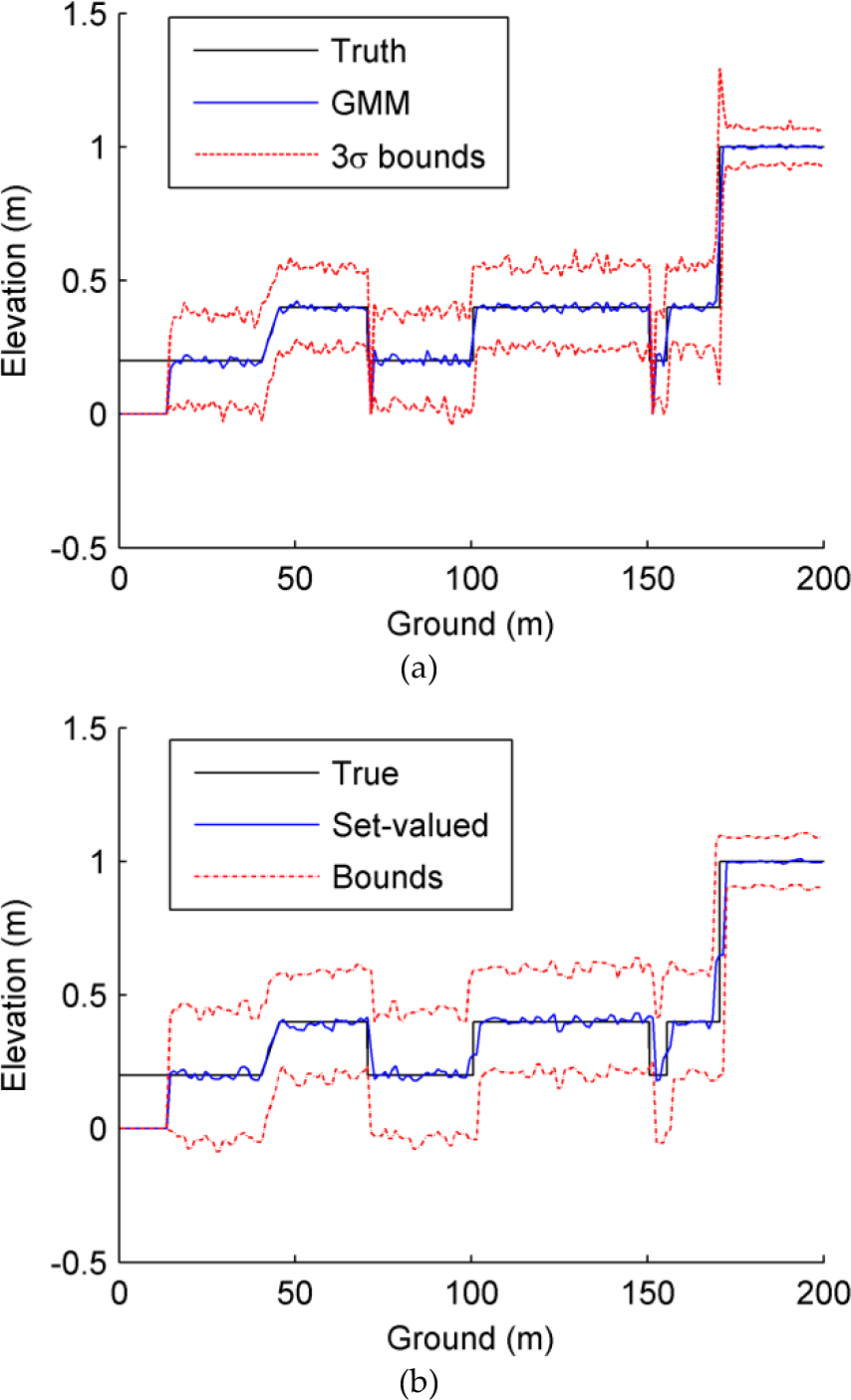
2D terrain estimation under Gaussian noise: (a) GMM, and (b) set-valued

The measurement model can be created as:

x = f (p, r) = (\begin{matrix} r \cos ϕ + x \\ r \sin ϕ + h_{m} \end{matrix})

(25)

with the model parameter p = [x φ]^T. The inclusion function is selected as follows to satisfy the condition of Lemma 1:

[x] = (\begin{matrix} [r] \cos [ϕ] + [x] \\ [r] \sin [ϕ] + h_{m} \end{matrix})

(26)

Two kinds of uncertainty assumptions will be considered: i) Gaussian noises with 3σ bounds δ_p = [δ_x δ_φ]^T and δ_r; ii) uniformly-distributed noises with hard bounds δ_p and δ_r. The covariances of the GMM algorithm are set to Q_p = diag[(δ_x/3)², (δ_φ/3)²]^T, Q_r = (δ_r/3)². The results for GMM and the set-valued terrain estimation algorithms under different uncertainties are depicted in Figures 3 and 4.

Figure 4.

2D terrain estimation under bounded noise: (a) GMM, and (b) set-valued

In simulations, the 3σ bounds of the GMM terrain estimation are drawn to describe the estimation uncertainties. For the set-valued algorithm, although all the points in the estimated terrain interval have the same “probabilities” to stand for the true terrain features, the centre of the interval is chosen as the referenced point estimation of the terrain. At the beginning of the terrain, no estimation is produced because the terrain at that point cannot be sensed by the LRF. It can be seen from the figures that both algorithms can track slow-varying continuous terrains (flat terrains and slopes) very well, while the set-valued algorithm gives strict confidence bounds of the terrain with respect to the probabilistic uncertainty bounds of the GMM algorithm. The set-valued algorithm can produce a much smoother terrain estimation than the GMM algorithm, especially at those places that cannot be sensed because of occlusions - that is, at the points x = 70.5 m and 155.5 m, where burrs will occur for the terrain estimated by the GMM algorithm. This is a benefit of the inherent conservation and robustness of the set-valued algorithm, which provide a potential terrain-filtering mechanism with the ability to fill gaps in the map. Moreover, and as for the vertical wall at x = 170.5 m where a big sudden change happens, the bounds obtained by the GMM algorithm expanded quickly due to increasing uncertainties caused by the fusions of large amounts of distinct measurements to give a dominant elevation. In contrast, the set-valued algorithm can remove this drawback by providing the terrain variation bounds in order to represent multi-elevation terrains in a cell.

In addition, other performance comparisons of the two algorithms, such as the CPU time and the root mean square error (RMSE) of the terrain estimation defined as:

RMSE = \sqrt{\sum_{i = 1}^{N} {({\hat{z}}_{i} - z_{i})}^{2} / N}

(27)

where z_i and ẑ_i are the true and estimated terrain data for each cell, are listed in Table 1.

Table 1.

Comparisons of terrain estimations

	GMM		Set-valued
	Time (ms)	RMSE	Time (ms)	RMSE
Gaussian noises	0.1583	0.0124	0.0610	0.0185
Bounded noises	0.1602	0.0135	0.0612	0.0086

With Gaussian noises, the RMSE of the GMM algorithm turns out to be better than the set-valued algorithm because the Gaussian uncertainties assumption is satisfied. However, for uniformly-distributed bounded noise that violates the Gaussian noise assumption, the performance of the GMM approach degenerates significantly while the set-valued approach can provide superior estimations, even better than its own results under Gaussian noise. This shows the effectiveness of the set-valued algorithm, with greater robustness for different noise assumptions. For CPU time costs, the set-valued algorithm is over 60% faster than the GMM algorithm for each iteration step under both noise assumptions, which guarantees the real-time performance of our proposed algorithm. It should also be noted that although the centres of the estimated sets for the set-valued approach are given here as point estimations, the terrain bound is more significant because the aim of the set-valued approach is to produce a terrain variation representation for multi-elevation terrains.

6. Experiments

In this section, we performed an experimental validation of our proposed terrain estimation algorithm in outdoor environments with a tracked mobile robot, as shown in Figure 5.

Figure 5.

The experimental tracked robot

The size of the robot is b = 0.65 m and R = 0.35 m. A SICK LMS221 2D scanning laser is mounted on the robot at a height of h_m = 0.468 m. The scanning angle of the laser is denoted by θ. The fixed pitch angle between the scanning plane and the horizontal plane is set to φ = −10°. Other sensors mounted on the robot include the encoders of two wheels that drive the tracks, two ADXL203 accelerometers, a 2DOF electric tilt sensor, a gyroscope and a GPS, which are adopted given low cost considerations for the outdoor 3D localization of the robot.

The measurement model of the scanning laser is derived as:

x = f (p, r) = (\begin{matrix} x_{r} + r \cos θ \\ y_{r} + r \sin θ \cos ϕ \\ h_{m} + r \sin θ \sin ϕ \end{matrix})

(28)

with the coordinates transformations:

T_{2} (p_{r}) = (\begin{matrix} I_{3 \times 3} & p_{r} \\ 0 & 1 \end{matrix})

(29)

T_{1} (φ) = (\begin{matrix} 1 & 0 & 0 & 0 \\ 0 & \cos ϕ & - \sin ϕ & 0 \\ 0 & \sin ϕ & \cos ϕ & h_{m} - z_{r} \\ 0 & 0 & 0 & 1 \end{matrix})

(30)

R (r) = {(\begin{matrix} r \cos θ & r \sin θ & 0 & 1 \end{matrix})}^{T}

(31)

where R, T₁ and T₂ are transformation matrices of four coordinate frames: the polar coordinates frame for laser scanning, the laser coordinates frame, the robot coordinates frame and the global coordinates frame. In addition, p = (x, y, φ, θ)^T is the model parameter and r is the measurement. The robot position p _r = (x_r, y_r, z_r)^T is given by the set-membership-based pose estimation algorithm with the uncertainties δ_x, δ_y and δ_z. The uncertainty of φ is set to δ_φ, = 0.5° according to the calibration average values. The uncertainty of the laser scanning angle is set to δ_θ = 0.24°. The uncertainty of the laser measurement is δ_r = 0.02 m, according to the accuracy of the laser. The inclusion function is selected as follows to satisfy the condition of Lemma 1:

[x] = (\begin{matrix} [x_{r}] + [r] \cos [θ] \\ [y_{r}] + [r] \sin [θ] \cos [ϕ] \\ [h_{m}] + [r] \sin [θ] \sin [ϕ] \end{matrix})

(32)

In order to improve the localization accuracy and pay more attention to the terrain estimation algorithm itself, the robot is set to run on the passage road at a slow speed of about 10 cm/s. The pose of the robot is estimated by SMF - as in [25] - with odometer data.

In the experiments, the GMM algorithm and our proposed set-valued algorithm are compared. The Gaussian noise covariance of the GMM algorithm is selected as Q_p=diag[(δ_x/3)², (δ_y/3)², (δ_φ/3)², (δ_θ/3)²]^T, Q_r=(δ_r/3)².

Two experimental scenes are tested and compared. The first experimental scene is constructed by stairs with a height of 14 cm and a width of 34 cm (see Figure 6). The laser is set to scan on a plane with a resolution of 180§/0.25° and a frequency of 100 Hz, where the scanning angle is denoted by θ. The cell size is chosen as 5 cm. The results for the terrain estimation of the two algorithms are displayed in Figure 7, with the bound estimation at lines x = 1 m being shown in Figure 8. Here, the bound of the GMM algorithm is chosen as the 3σ bound of the elevation estimation, while the terrain point estimation of the set-valued algorithm is chosen as the centre of the interval.

Figure 6.

Stair terrain for the experiment

Figure 7.

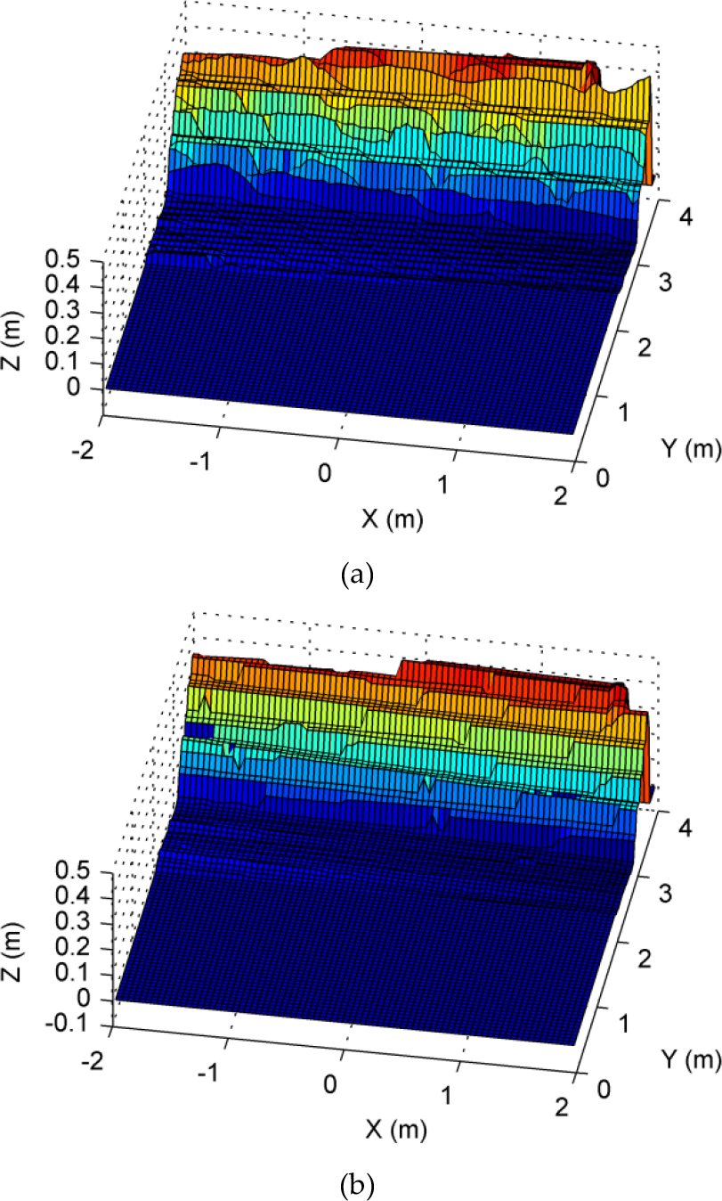
3D terrain estimation results: (a) GMM, and (b) set-valued

Figure 8.

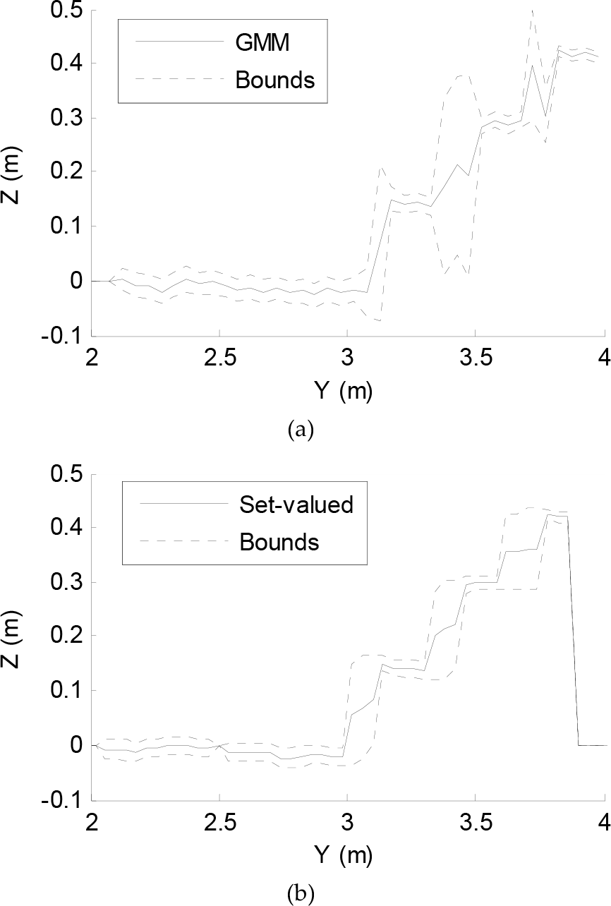
Terrain estimation at x = 1 m: (a) GMM, and (b) set-valued

From these figures, it can be easily seen that the terrain map produced by the set-valued algorithm is much smoother, especially when sudden changes in the terrain occur, such as with the vertical structures at about y = 3 m, 3.3 m and 3.7 m in Figure 8. With the GMM results, abrupt bounds changes have happened for these locations. Meanwhile, with the set-valued results, the estimated bounds are smoother and seem more conservative. It can also be seen that in Figure 7 there are many irregular cuts (or ‘patches’) in each layer of the GMM terrain, while in the set-valued terrain the terrain estimation is much more regular. That is, the latter benefits from the potential terrain filtering ability introduced by the conservativeness of the set-theoretic frameworks. Note that the heading of the robot is not perpendicular to the stairs, and therefore the terrain produced in the two algorithms may be divided into several parts.

Another advantage introduced by the set-valued algorithm lies in the smoother bounds estimation as compared to the GMM algorithm - as can be seen in Figure 8 - which provides for a greater confidence in the terrain variation for multi-elevation terrain along with the greater robustness of the algorithm. The real terrain (with a height of 14 cm and a width of 34 cm) can thus be bounded by set-valued bounds but not by GMM bounds.

However, the smoothness of the terrain may cause erroneous point-estimation - as can be seen in Figure 8 -while the stairs seem more like segmented slopes rather than actual stairs, which indicates the trade-off between terrain filtering and real sudden change detection. For structured environments, the octree-based method may be more accurate than the probabilistic algorithm. The biggest advantage of the set-valued algorithm is that it can provide conservative but correct bound estimations. In fact, in the set-valued algorithm the bound estimation is more important than the point-value estimation because all the points in a given feasible set have the same probability of occurrence.

As for real-time performance, the time cost of the set-valued algorithm is 87.6 ms for each step - about 44.4% faster than 157.5 ms of the GMM algorithm. Note that the real-time improvement gained here is not the same as with the simulation results, because the time cost also depends on the bounds of the uncertainties that determine the updating area of the elevation model as discussed above, which means that more accurate laser sensors or localization methods will result in less computational time.

The second experimental scene is a complex snow terrain of about 4 m × 6 m with a passage surrounded by two snow walls, as shown in Figure 9. The laser is set to scan on a plane with a resolution of 180°/1° with a frequency of 50 Hz. In this experiment, the ground is highly unstructured and uncertain, so the bounds of the terrain are more important than the point estimation.

Figure 9.

Snow terrain for the experiment

The cell size is chosen as 10 cm. The results for the terrain estimation of the two algorithms are shown in Figure 10, with the bound estimations at lines x = 0 m, 0.8 m and −0.8 m being shown in Figures 11 –13.

Figure 10.

3D terrain estimation results: (a) GMM, and (b) set-valued

Figure 11.

Terrain estimation at x = 0 m: (a) GMM, and (b) set-valued

Figure 12.

Terrain estimation at x = 0.8 m: (a) GMM, and (b) set-valued

Figure 13.

Terrain estimation at x = −0.8 m: (a) GMM, and (b) set-valued

From these figures of the snow terrain, it can also be seen that the terrain map produced by the set-valued algorithm is much smoother, such as with the vertical structures at about y = 4 m in Figure 11 and y = 1.4 m in Figure 12. Moreover, the gaps that arise from laser data loss due to the occlusions or outliers can be filled by the set-valued algorithm. For example, in the cells between y = 4.5 m and y = 5.5 m of Figure 11, where the terrain is occluded by a large obstacle that cannot be manoeuvred by the robot, a peak appears at y = 4.6 m for the GMM algorithm, while in set-valued algorithm this erroneous estimation is corrected and a smaller terrain blank from the occlusion is created. A similar situation can be seen between y = 0.8 m and 1.5 m in Figure 12. The smoother bounds estimation of the set-valued algorithm when compared to the GMM algorithm can also be seen in all these figures. As for real-time performance, the time cost of the set-valued algorithm is 39.6 ms for each step - about 42.2% faster than the 68.5 ms of the GMM algorithm.

The above analysis shows that the set-valued terrain estimation algorithm often leads to better performance for complex outdoor terrain environments, especially for highly unstructured terrain environments (rough terrain) with frequent terrain changes, which result in multi-elevation cells (as the snow terrain used here shows). The gaps may be filled to make the terrain smoother. Moreover, the traditional elevation map with a single dominant elevation for each cell cannot give a correct terrain representation, while the set-valued algorithm can provide an elevation variation range that can be used to evaluate the roughness of the terrain. However, for structured environments such as stairs, the filtering efficiency may lead to erroneous point estimations of the terrain, just as is the case with the traditional probabilistic algorithm. So, the trade-off between terrain filtering and real terrain estimation should be carefully considered when our algorithm is used in structured environments. It is more important that the set-valued algorithm can still provide conservative but correct bounds estimations when compared to probabilistic algorithms. In addition, the lower computational time required makes the algorithm more suitable for real-time applications, especially for large-scale, rough terrain environments.

7. Conclusions

In this paper, a uniform set-theoretic framework is used to model outdoor rough and unstructured terrains by a set-valued elevation map that extends the concept of the traditional elevation map in the following aspects: i) uncertainties coming from multiple sources, such as sensor accuracy and the calibration error of the sensor platform or the localization error of the robot, are considered and processed uniformly as the UBB errors, which provide a more practical alternative to the probabilistic distribution assumptions with increased robustness; ii) all the measurements are processed iteratively to create the set-valued elevation map by propagating UBB uncertainties into the map through transformation, association and fusion. The simultaneous localization problem is also solved under the set-theoretic framework to give the guaranteed bounded pose estimation consistent with the UBB assumption. The set-valued terrain model can provide terrain variation range for each cell, which can be used to evaluate the terrain roughness constraints for successive planning and control tasks; iii) the set-valued algorithm maintains a good balance between the richness of the terrain model and computational complexity, which makes it more suitable for real-time applications. Moreover, a potential terrain filtering effect can be achieved to introduce greater smoothness for the terrains by the inherent conservativeness of the algorithm, which is more suitable for rough outdoor terrain. Future works include large-scale environmental tests of our algorithm to demonstrate its efficiency and adaptability for several typical outdoor applications, and further the development of the set-valued terrain estimation algorithm to construct a more complicated environment model comprising multi-level terrain features such as tunnels, trees, bridges, and so on. Moreover, explorations should be done to incorporate the proposed terrain estimation algorithm with path planning and configuration adjustment problems, which will enable the robot to manoeuvre over rough terrains with high stability, superior reliability and a lower power consumption.

Footnotes

8. Acknowledgments

This work is supported by the National Natural Science Foundation of China (Grant Nos. 61005092, 61105094) and the Research Fund for the Doctoral Programme of Higher Education of China (20100092120026).

References

Almazan

C B

Youssef

Aqrawala

A K

(2007) Rover: An integration and fusion platform to enhance situational awareness. In Proceedings of IEEE International Performance Computing and Communications Conference, New Orleans, Louisiana, pp. 582–587.

Vasudevan

Ramos

Nettleton

Durrant-Whyte

(2009) Gaussian process modeling of large-scale terrain. Journal of Field Robotics, 26 (10): pp. 812–840.

Matthies

Xiong

Hogg

(2002) A portable, autonomous, urban reconnaissance robot. Robotics and Autonomous Systems, 51 (2): pp. 163–172.

Nicosevici

Gracias

Negahdaripour

Carcia

(2009) Efficient three-dimensional scene modeling and mosaicing. Journal of Field Robotics, 26 (10): pp. 759–788.

Papadakis

(2013) Terrain traversability analysis methods for unmanned ground vehicles: a survey. Engineering Applications of Artificial Intelligence, 26: 1373–1385.

Elfes

(1989) Using occupancy grids for mobile robot perception and navigation. Computer, 22 (6): pp. 46–57.

Moravec

H P

(1996) Robot spatial perception by stereoscopic vision and 3d evidence grids. Technical Report CMU-RI-TR-96–34, Carnegie Mellon University, Robotics Institute.

Tirumalai

A P

Schunck

B G

Jain

R C

(1995) Evidential reasoning for building environment maps. IEEE Transactions on Systems, Man and Cybernetics, 25 (1): pp. 10–20.

Pagac

Nebot

E M

Durrant-Whyte

(1998) An evidential approach to map-building for autonomous vehicles. IEEE Transactions on Robotics and Automation, 14 (4): pp. 623–629.

10.

Roth

Wibowoo

(1997) An efficient volumetric method for building closed triangular meshes from 3D image and point data. In Proceedings of the Conference on Graphics Interface, Kelowna, Canada, pp. 173–180.

11.

Thrun

Martin

Liu

Hahnel

Emery

Montemerlo

Chakrabarti

Burgard

(2004) A real-time expectation-maximization algorithm for acquiring multiplanar maps of indoor environments with mobile robots. IEEE Transactions on Robotics and Automation, 30 (3): pp. 433–442.

12.

Ryde

(2010) 3D mapping with multi-resolution occupied voxel lists. Autonomous Robots, 28 (2): pp. 169–185.

13.

Wurm

K M

Hornung

Bennewitz

(2010) OctoMap: A probabilistic, flexible, and compact 3D map representation for robotic systems. In Proceedings of IEEE International Conference on Robotics and Automation, pp. 12–24.

14.

Hoffman

Krotkov

(1992) Terrain mapping for long-duration autonomous walking. In Proceedings of International Conference on Intelligent Robots and Systems, Raleigh, NC: IEEE, 1: pp. 563–568.

15.

Hygounenc

Jung

I K

Soueres

Lacroix (2004) The autonomous blimp project of laas-cnrs: achievements in flight control and terrain mapping. International Journal of Robotics Research, 23 (4–5): pp. 473–511.

16.

Borenstein

(2004) A novel filter for terrain mapping with laser rangefinders. IEEE Transactions on Robotics and Automation, 20 (5): pp. 913–921.

17.

Miller

Campbell

(2006) A mixture-model based algorithm for real-time terrain estimation. Journal of Field Robotics, 23 (9): pp. 755–775.

18.

Kleiner

Dornhege

(2007) Real-time localization and elevation mapping within urban search and rescue scenarios. Journal of Field Robotics, 24 (8–9): pp. 723–745.

19.

Pfaff

Triebel

Burgard

(2007) An efficient extension of elevation maps for outdoor. The International Journal of Robotics Research, 26 (2): pp. 217–230.

20.

Rivadeneyra

Miller

Schoenberg

J R

Campbell

(2009) Probabilistic estimation of multi-level terrain maps. In Proceedings of IEEE International Conference on Robotics and Automation, pp. 1643–1648.

21.

Vasudevan

Ramos

Nettleton

Durrant-Whyte

(2011) Non-stationary dependent Gaussian processes for data fusion in large-scale terrain modeling. In Proceedings of the 2011 IEEE /RSJ International Conference on Intelligent Robots and Systems (IROS), San Francisco, California, USA, pp. 440–445.

22.

Zhou

Dai

X Z

(2010) Set-membership based real-time terrain modeling of mobile robots with a laser scanner. In Proceedings of the 2010 IEEE International Conference on Mechatronics and Automation (ICMA), Xi'an, China, pp. 440–445.

23.

Leal

(2003) Stochastic environment representation. Ph. D. thesis, University of Sydney, Australian Centre for Field Robotics.

24.

Nuchter

Lingemann

Hertzberg

Surmann

(2007) 6D SLAM-3D mapping outdoor environments: research articles. Journal of Field Robot, 24 (8–9): pp. 699–722.

25.

Weingarten

Siegwart

(2005) EKF-based 3D SLAM for structured environment reconstruction. In Proceedings of the IEEE/RSJ International Workshop on Intelligent Robots and Systems, Los Alamitos: Institute of Electrical and Electronic Engineers, pp. 3834–3839.

26.

Zhou

Han

J D

Liu

G J

(2008) A UD factorization-based nonlinear adaptive set-membership filter for ellipsoidal estimation. International Journal of Robust and Nonlinear Control, 18 (16): pp. 1513–1531.

27.

Moore

R E

(1997) Methods and applications of interval analysis. SIAM Publisher: Philadelphia, PA.

28.

Durrant-Whyte

Bailey

(2006) Simultaneous localization and mapping: part I the essential algorithm. IEEE Robotics and Automation Magazine, 13 (2): 99–110.

29.

Jaulin

Kieffer

Didrit

Walter

(2001) Applied interval analysis, 1st ed. London, Great Britain: Springer-Verge.

30.

Scholte

Campbell

M E

(2003) A nonlinear set-membership filter for on-line applications. International Journal of Robust and Nonlinear Control, 13: pp. 1337–1358.

31.

Zemke

b4m: a free interval arithmetic toolbox for matlab, http://www.ti3.tuhh.de/zemke/b4m/, version 1.0.2.004.

A Set-Theoretic Algorithm for Real-Time Terrain Mapping of Mobile Robots in Outdoor Environments

Abstract

Keywords

1. Introduction

2. Problem formulation

3. Set-theoretic terrain estimation

3.1 Elevation modelling

3.2 Measurements modelling and transformation

3.3 Elevation assignment

3.4 Elevation fusion and map updating

3.5 Algorithm summary

4. Set-membership-based localization

5. Simulations

6. Experiments

7. Conclusions

Footnotes

8. Acknowledgments

References