A terrain description method for traversability analysis based on elevation grid map

Abstract

Terrain traversability analysis is a challenging problem for mobile robots to adapt to complex environments, including the detection of cluttered obstacles, potholes, or even slopes. With the accurate distance information, using distance sensors such as three-dimensional light detection and ranging (LiDAR) for terrain description becomes a preferred choice. In this article, a terrain description method for traversability analysis based on elevation grid map is presented. After the elevation grid map is generated, the ground is segmented with the aid of a height difference kernel and the non-ground grids in the map are then clustered. The terrain description features, including height index, roughness, and slope angle, are calculated and estimated. The slope angle is estimated using random sample consensus (RANSAC) and least squares method, and specifically, the roughness is combined to eliminate false slopes. Experimental results verified the effectiveness of the proposed method.

Introduction

Terrain traversability analysis ¹ is an important and challenging problem for mobile robots. To acquire the terrain information, the sensors such as stereovision, three-dimensional (3-D) light detection and ranging (LiDAR) have been adopted to provide original point cloud.

Some researchers address the problem based on original point cloud. Akdeniz and Bozma ² presented an approach to local terrain mapping using bubble space representation, where the bubble surfaces are constructed using 3-D laser data. Dargazany and Berns ³ presented a stereo-based superpixel surface approach for terrain traversability analysis of unmanned ground vehicles. Geometry-based features (pixel-based normal) are used to detect all the existing surfaces. Then, superpixel surface analysis is applied on these surfaces to classify them into five categories based on their traversability index. Still, the data processing including stereo matching and point cloud generation is time-consuming. Bellone et al. ^{4 –6} presented unevenness point descriptor (UPD) for terrain analysis. It uses principal component analysis (PCA) to estimate normal vectors of query points, and then UPD is given by these normal vectors. Lalonde et al. ⁷ proposed a 3-D data segmentation method for terrain classification. The “scatter,” “linear,” and “surface” objects can be classified with a Gaussian mixture model and a Bayesian classifier.

Obviously, directly applying these raw point cloud data shall increase the complexity of data processing. In this case, grid maps provide an effective solution. Belter and Skrzypczyński. ⁸ presented an algorithm for real-time building of a local grid-based elevation map from noisy two-dimensional range measurements. The terrain mapping supports a foothold selection for a walking robot based on grid level. More terrain analysis is not mentioned. Neuhaus et al. ⁹ presented a grid-based algorithm for classifying regions as either drivable or not. The local terrain roughness feature based on PCA is estimated for terrain drivability analysis. Reddy and Pal. ¹⁰ proposed a measure of terrain unevenness by computing ranges of neighboring laser beams of a 3-D laser scanner. The unevenness analysis forms an unevenness field around the robot. A traversable region can be marked out by setting thresholds on unevenness in order to detect obstacles. Tanaka et al. ¹¹ proposed a terrain traversability analysis method for mobile robot navigation. With the roughness and slope features extracted from the grid map, they adopted fuzzy inference to calculate the traversability of the rectangular areas to generate a drivable direction.

It shall be noted that terrain description based on the map with grid-level analysis often focuses on the problem of whether the grid is traversable or not. On the one hand, there are some other terrain information such as slopes that should be described. On the other hand, for the grid map, grid-level analysis is a little trivial, and cluster-level analysis is preferable. Jin et al. ¹² presented a method for traversability analysis, which extracts slope and roughness of a terrain patch along four heading directions and then uses them to evaluate the level of difficulty associated with the traversal. The slope is estimated by least squares method and the roughness is also obtained. Gu et al. ^13,14 proposed a traversability approach based on an extended 2.5-D grid-based representation of the rough terrain using stereovision and omnidirectional vision sensors. Height difference, slope, and roughness are considered as terrain properties to assess the traversability, and a fuzzy logic framework is applied to extract traversability indices from terrain characteristics. Ye et al. ^{15 –17} constructed a polar traversability index (PTI) to evaluate terrain traversal property, which indicates the level of difficulty for a robot to move along the corresponding direction. Slope and roughness of each terrain patch are estimated through least-squares plane fitting.

It shall be noted that an advantage of 3-D LiDAR is to directly provide accurate distance information. With this advantage, we conduct the research on terrain description. In this article, a terrain description method for traversability analysis based on elevation grid map is presented. The slope angle is estimated using RANSAC and least squares method, and the roughness feature is adopted to eliminate false slopes. The effectiveness of this terrain description method is verified by experiments.

Elevation grid map

The point cloud data to acquire terrain information are from a 3-D LiDAR. The coordinate systems O_LX_LY_LZ_L and O_RX_RY_RZ_R are established as shown in Figure 1, where O_LX_LY_LZ_L refers to LiDAR coordinate system and O_RX_RY_RZ_R is the robot coordinate system.

Figure 1.

Coordinate systems.

Based on the raw point cloud data, the transformed point cloud data set D_P in O_RX_RY_RZ_R can be acquired with the help of external parameters calibration. ¹⁸ Then, the elevation grid map M is generated with D_P , and each grid in M can be defined as c_{l ,w} , where l and w are the integer coordinates of this grid in M. The coordinate system O_MX_MY_M is established to describe M, where O_M is the center of M whose length and width are expressed by L and W, respectively. Figure 2 illustrates the elevation grid map M. For each point p_i(x_i, y_i, z_i) in D_p , it will be projected into the grid c_{l ,w} in M if the following equation is satisfied

$p_{l,w}=\left\{p_i\left(x_i,y_i, z_i\right)\right\}$

$p_i\in D_P$

$0\le l=\lfloor \left(x_i+L/2\right)/c_{\text{size}}\rfloor <L/c_{\text{size}}$

$0\le w=\lfloor \left(y_i+W/2\right)/c_{\text{size}}\rfloor <W/c_{\text{size}}$

Figure 2.

Illustration of the elevation grid map.

where p_{l ,w} is the point cloud data set of the points in D_P that are projected into c_{l ,w} in M, and c_size refers to the side length of each grid in M.

It can be found that $p_{l,w}\subseteq D_P$ , and p_{l ,w} can be φ if no points are projected into c_{l ,w} , where φ is the empty set. The relationship between p_{l ,w} and c_{l ,w} is illustrated in Figure 2. The data points in D_P will not be considered if their integer coordinates of corresponding grids are out of range.

The height attributes of each c_{l ,w} , including maximum height, ¹⁵ minimum height, mean height, ¹³ and height difference, ¹⁹ are necessary features for elevation grid map, which should be calculated based on its corresponding p_{l ,w} . For each p_{l ,w} , the maximum height and the minimum height are labeled as $h_{l,w}^{\text{max}}$ and $h_{l,w}^{\text{min}}$ , respectively. And the mean height $h_{l,w}^{\text{mean}}$ is the average height of all the points in p_{l ,w} . Obviously, the height difference of all the points in p_{l ,w} can be obtained as $h_{l,w}^{\text{diff}}=h_{l,w}^{\text{max}}-h_{l,w}^{\text{min}}$ . Notice that these height-related attributes $h_{l,w}^{\text{max}}$ , $h_{l,w}^{\text{min}}$ , $h_{l,w}^{\text{mean}}$ , and $h_{l,w}^{\text{dif}f}$ are also attached to the grid c_{l ,w} . By this way, the elevation grid map is generated.

Terrain description based on elevation grid map

After the elevation grid map is generated, the terrain can be subdivided into different types, including obstacles, potholes, slopes, and so on. Grids in the elevation grid map shall be clustered after ground segmentation is finished. And then, the terrain description features including height index H_f , roughness R_n , and slope angle α_s are introduced in details, which pave the foundation of terrain description.

Ground segmentation

There are many grids belong to the ground in M, which should be eliminated first to reduce the computational complexity. Height information in the elevation grid map provides an effective solution for ground segmentation. In this article, multiple height information is utilized for height description to detect non-ground grids as many as possible. For the grid c_{l ,w} , it is marked as a non-ground grid if the following equation is satisfied

$\begin{array}{l}{C}_N=\left\{c_{l,w}\right|(h_{l,w}^{\text{dif}f}\ge T_{\text{diff}})\cup \\ (h_{l,w}^{\text{max}}\ge T_{\text{high}})\cup (h_{l,w}^{\text{min}}\le T_{\text{low}})\}\end{array}$

1

where T _diff, T _high, and T _low are given thresholds, and C_N is the non-ground grids set. Then, the set of ground grids is easily obtained and it is expressed by C_G .

Notice that there are also some grids with small height values, which may be mistaken as ground grids according to equation (1). To solve this problem, a height difference kernel is exerted on the set C_G . The kernel adopts not only the height information of the grid but also the height information from its neighboring grids. For a specific ground grid c_{l ,w} in C_G , it will be removed from the set C_G and added to the non-ground grids set C_N if equation (2) is satisfied

${\displaystyle \sum _{s=-a}^a{\displaystyle \sum _{t=-b}^{b}w(s,t)\cdot h_{l+s,w+t}^{\text{mean}}}}\ge T_{\text{diff}}$

2

where w(s, t) is the neighboring height difference kernel (see Figure 3), w(0, 0) is the value of its center grid in the kernel, a = 1, b = 1, and $h_{l+s,w+t}^{\text{mean}}$ is the mean height of the ground grid c_{l + s , w + t} in C_G .

Figure 3.

The neighboring height difference kernel with an 8-connected domain.

If the grid c_{l ,w} is filled to the set C_N , the mean height of c_{l ,w} shall be increased to T _high. It should be noted that this kernel processing only examines the ground grids in C_G that have eight neighboring ground grids.

Algorithm 1

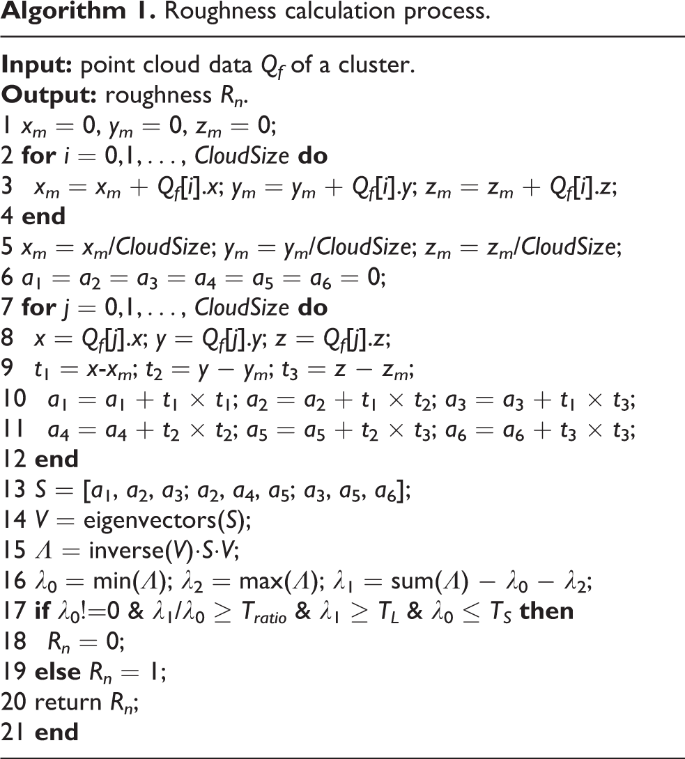
Roughness calculation process.

Input: point cloud data Qf of a cluster.

Output: roughness Rn .

1 xm = 0, ym = 0, zm = 0;

2 for i = 0,1,…, CloudSize do

3  xm = xm + Qf [i].x; ym = ym + Qf [i].y; zm = zm + Qf [i].z;

4 end

5 xm = xm /CloudSize; ym = ym /CloudSize; zm = zm /CloudSize;

6 a 1 = a 2 = a 3 = a 4 = a 5 = a 6 = 0;

7 for j = 0,1,…, CloudSize do

8  x = Qf [j].x; y = Qf [j].y; z = Qf [j].z;

9  t 1 = x-xm ; t 2 = y − ym ; t 3 = z − zm ;

10  a 1 = a 1 + t 1 × t 1; a 2 = a 2 + t 1 × t 2; a 3 = a 3 + t 1 × t 3;

11  a 4 = a 4 + t 2 × t 2; a 5 = a 5 + t 2 × t 3; a 6 = a 6 + t 3 × t 3;

12 end

13 S = [a 1, a 2, a 3; a 2, a 4, a 5; a 3, a 5, a 6];

14 V = eigenvectors(S);

15 Λ = inverse(V)·S·V;

16 λ 0 = min(Λ); λ 2 = max(Λ); λ 1 = sum(Λ) − λ 0 − λ 2;

17 if λ 0!=0 & λ 1/λ 0 ≥ Tratio & λ 1 ≥ TL & λ 0 ≤ TS then

18  Rn = 0;

19 else Rn = 1;

20 return Rn ;

21 end

Grids clustering

Flood fill algorithm ²⁰ is used to integrate the non-ground grids in C_N that are adjacent in eight directions into the same cluster, as shown in Figure 4. The clusters that contain less than T_c grids shall be directly eliminated, where T_c is a given threshold. Notice that the point cloud data sets corresponding to the non-ground grids are also integrated.

Figure 4.

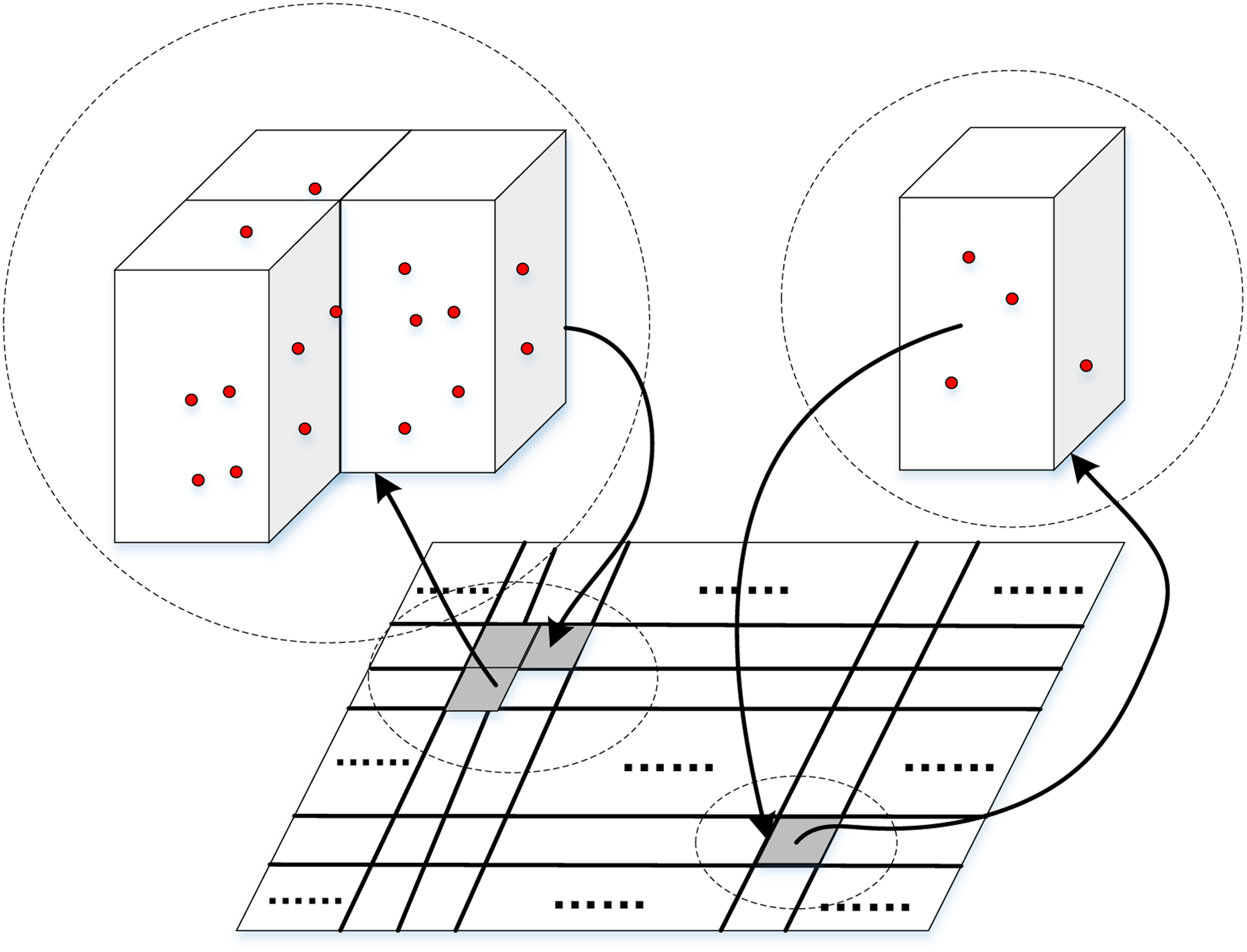
Non-ground grids clustering based on the elevation grid map.

Terrain description features

Based on these clustered grids and their corresponding clustered point cloud data, the terrain description features are addressed. Three features are chosen to describe the cluster-based terrain, and they are height index H_f , roughness R_n , and slope angle α_s . H_f stands for the height information of a cluster. The unevenness degree of a cluster is reflected by R_n , and α_s represents the steepness degree of a cluster.

Among the height features, the value of maximum height feature is easy to be changed due to robot motion, and the mean height feature cannot reflect the height range of the cluster. In contrast, height difference is a robust height feature for mobile robots. However, it cannot distinguish clusters of point cloud with large heights but small height differences. In this article, height index H_f based on the height attributes of all c_{l ,w} in a cluster is introduced, which is a combination of the height-related attributes

$\begin{array}{l}{H}_f=\{\begin{array}{c}\text{max}\{H_d,H_m\},(H_m>0)\\ \text{min}\{-H_d,H_m\},(H_m<0)\end{array}\\ H_d=H_{\text{max}}-H_{\text{min}},H_m=\frac{1}{n_c}{\displaystyle \sum _{k=1}^{n_c}{h}_k^{\text{mean}}}\end{array}$

3

where H_d is the height difference of this cluster, H_m is the mean height of this cluster, $H_{\text{max}}=\text{max}\left\{h_k^{\text{max}}\right|k=1,2,\dots ,n_c\}$ , $H_{\text{min}}=\left\{h_k^{\text{min}}\right|k=1,2,\dots ,n_c\}$ , $h_k^{\text{max}}$ is the kth grid’s maximum height, $h_k^{\text{min}}$ is the kth grid’s minimum height, $h_k^{\text{mean}}$ is the kth grid’s mean height, and n_c is the size of grids in the cluster.

Algorithm 2

Slope angle estimation process.

Input: point cloud data Qf of a cluster

Output: slope angle αs .

1 NumofInliers = 0; BestInliers = NULL;

2 for i = 1,2,…, MaxIterations do

3  n 1 = rand(), n 2 = rand(), n 3 = rand();

4  p 1 = Qf [n 1], p 2 = Qf [n 2], p 3 = Qf [n 3];

5  Ai = (p 2.y − p 1.y) × (p 3.z − p 1.z) − (p 3.y − p 1.y) × (p 2.z − p 1.z);

6  Bi = (p 3.x − p 1.x) × (p 2.z − p 1.z) − (p 2.x − p 1.x) × (p 3.z − p 1.z);

7  Ci = (p 2.x − p 1.x) × (p 3.y − p 1.y) − (p 2.y − p 1.y) × (p 3.x − p 1.x);

8  Di = −Ai *p 1.x − Bi *p 1.y − Ci *p 1.z;

9  for j = 0,1,…, CloudSize do

10  distancej = PointToPlaneDistance(Qf [j], Ai , Bi , Ci , Di );

11  if distancej ≤ TSegment then

12  inliers.push_back(j);

13  end

14 end

15 if inliers.size() ≥ NumofInliers then

16  NumofInliers = inliers.size();

17  BestInliers = inliers;

18 end

19 if NumofInliers/CloudSize > TInlier then

20  break;

21  end

22 end

23 a 1 = a 2 = a 3 = a 4 = a 5 = 0; b 1 = b 2 = b 3 = 0;

24 for k = 0,1,…, nt do

25  x = inliers[k].x; y = inliers[k].y; z = inliers[k].z;

26  a 1 = a 1 + x 2; a 2 = a 2 + xy; a 3 = a 3 + x;

27  a 4 = a 4 + y 2; a 5 = a 5 + y; a 6 = nt ;

28  b 1 = b 1 + zx; b 2 = b 2 + zy; b 3 = b 3 + z;

29 end

30 MatA = [a 1, a 2, a 3; a 2, a 4, a 5; a 3, a 5, a 6];

31 VecB = [b 1, b 2, b 3];

32 VecC = MatA.svd(VecB);

33 αs = acos(1/sqrt(pow(VecC(0), 2) + pow(VecC(1), 2) + 1));

34 return αs .

Flat terrains and rough terrains have different distribution of point cloud so that we can deduce the rough degree of a terrain according to the distribution of its point cloud. PCA method ²¹ provides a solution to infer the point cloud distribution. Let’s consider the covariance matrix S of Q_f , where Q_f is a cluster of point cloud after filtering. It can be found that the eigenvectors of matrix S must be mutually orthogonal, because S is a real symmetrical matrix. In this case, the PCA of the covariance matrix S of Q_f is in fact equivalent to eigenvalue decomposition for S. ⁹ The eigenvectors and eigenvalues of S can be solved by singular value decomposition. S can be transformed into a diagonal matrix Λ with an invertible matrix V generated by these orthogonal eigenvectors, which is shown in the following

$\begin{array}{l}\Lambda =V^{-1}\cdot S\cdot V\\ S=\frac{1}{n_q}{\displaystyle \sum _{i=1}^{n_q}(q_i-\overline{q_c})\cdot {(q_i-\overline{q_c})}^T}\\ \overline{q_c}=\frac{1}{n_q}{\displaystyle \sum _{i=1}^{n_q}{q}_i}\end{array}$

4

where q_i is the ith point of Q_f , $\overline{q_c}$ is the calculated center point of Q_f , and n_q is the size of points in Q_f .

Obviously, the elements of diagonal matrix Λ are eigenvalues of S. That means the covariance in S is decoupled along three principal directions, which are defined by the eigenvectors of S. The sizes of eigenvalues indicate the distribution of the point cloud along these directions. If there exist two eigenvalues that are much larger than the third one, which means that there exist two main principal directions, the distribution of the point cloud is close to a plane. ⁷ Besides, the minimal eigenvalue and the median eigenvalue should satisfy the given thresholds. Define λ_k as the kth eigenvalue of S, and v_k as the kth eigenvector of S, where k ∈ {0, 1, 2}. Then, the roughness R_n of the cluster is given as follows. R_n is a Boolean variable and it is set to 0 when λ ₁ ≫ λ ₀, λ₁ ≥ T_L and λ₀ ≤ T_S, where λ₁ and λ₀ are the median value and the minimum value of three eigenvalues, respectively, T_L and T_S are given thresholds. The cluster of point cloud will be viewed as flat if R_n = 0, or else, it will be viewed as rough. Algorithm 1 gives the implementation of roughness calculation process in detail.

Compared with the methods that usually measure the vertical cross section of a slope to estimate its angle, ² the slope angle estimation through normal vector can reflect the global feature of a slope. In order to estimate normal vector of a cluster, many fitting methods can be adopted, such as least squares method and RANSAC family. Least squares method considers all the points in the point cloud to minimize the sum of the squares of the residuals. RANSAC algorithm ²² is a learning technique to estimate the parameters of the fitting plane by random sampling of observed data. Its goal is to maximize the size of inliers, which can be fitted into a hypothetical plane within a small error. However, both least squares method and RANSAC have disadvantages. The least squares method is easily to be trapped in local optimum and is vulnerable to interference, whereas the variances of the RANSAC estimation results are usually large. It should be noted that the estimation result of least squares method is accurate and stable if the point cloud data are clean enough, and RANSAC is more robust against the interference.

In this article, we propose a solution that combines the advantages of least squares method and RANSAC, where RANSAC is used for candidate points segmentation, and the least squares method is then used to estimate the normal vector with these candidate points. For a cluster, we assume that there exists a plane that contains as many points as possible within a given range of error. The hypothetical plane is illustrated in Figure 5, where the red points refer to the point cloud of the cluster.

Figure 5.

Illustration of the fitting plane and its normal vector.

This solution can be divided into three steps: plane segmentation, ²² normal vector estimation, and slope angle calculation. In the first step, the cluster of the point cloud Q_f will be divided into inliers and outliers, which is implemented through iterations. Three random points from Q_f are selected in the ith iteration, with which a plane S_i is generated as A_ix + B_iy + C_iz + D_i = 0. For each point in Q_f , if the distance between this point and S_i is within a given threshold T_q , this point will be added into the inliers set. The size of inliers set is counted in each iteration to find out the best plane parameters with maximum inliers ever reached. If the ratio of the inliers in Q_f reaches a given threshold or the iterations reach a given maximum number, the iterations will stop.

The second step is to estimate the normal vector for the inliers set segmented from Q_f . All the points in the inliers set will be considered for normal vector estimation. The plane to be generated can be expressed as z = A_nx + B_ny + D_n , where A_n , B_n , and D_n are plane coefficients that can be estimated by the least squares method as shown in the following

$\left(\begin{array}{ccc}{\displaystyle \sum _{k=1}^{n_t}{x}_k^2}& {\displaystyle \sum _{k=1}^{n_t}{x}_k{y}_k}& {\displaystyle \sum _{k=1}^{n_t}{x}_k}\\ {\displaystyle \sum _{k=1}^{n_t}{x}_k{y}_k}& {\displaystyle \sum _{k=1}^{n_t}{y}_k^2}& {\displaystyle \sum _{k=1}^{n_t}{y}_k}\\ {\displaystyle \sum _{k=1}^{n_t}{x}_k}& {\displaystyle \sum _{k=1}^{n_t}{y}_k}& n_t\end{array}\right)\left(\begin{array}{c}{A}_n\\ B_n\\ D_n\end{array}\right)=\left(\begin{array}{c}{\displaystyle \sum _{k=1}^{n_t}{x}_k{z}_k}\\ {\displaystyle \sum _{k=1}^{n_t}{y}_k{z}_k}\\ {\displaystyle \sum _{k=1}^{n_t}{z}_k}\end{array}\right)$

5

where x_k , y_k , and z_k are the coordinates of the kth point in the inliers set, and n_t is the size of inliers.

To solve equation (5), singular value decomposition is used. Then, the normal vector is acquired as $n_s=\left(A_n^{*}, B_n^{*},C_n^{*}\right)$ , which is the normalization of the plane’s normal vector (A_n , B_n , −1). The third step is to calculate the slope angle using n_s , as follows

${\alpha }_s=\text{\hspace{0.17em}arccos}(n_s\cdot n_v)$

6

where n_v is the normalized normal vector of X_RO_RY_R in O_RX_RY_RZ_R .

The entire slope angle estimation process can be described in Algorithm 2.

Terrain description

The terrain features including height index H_f , roughness R_n , and slope angle α_s can be used for terrain classification. In order to reduce the computational complexity, these three features are estimated in sequence. If H_f of a cluster is smaller than T _neg , it will be classified as a pothole, and the other two features will not be estimated for this cluster. The cluster of point cloud will be categorized as an obstacle if H_f is not less than T _pos with R_n = 1. In this case, it is not necessary to estimate α_s . Only when R_n = 0, α_s shall be considered. In actual applications, there usually exists an interval for the slope angle. For example, a wall is considered as an obstacle not a slope with α_s ≈ 90°. The abovementioned classification is summarized in Table 1, where T _pos and T _neg are given thresholds.

Table 1.

Terrain classification with terrain description features.

Type	Height index	Roughness	Slope angle
Pothole	Hf ≤ T neg	—	—
Obstacle	Hf ≥ T pos	Rn = 1	—
Slope	Hf ≥ T pos	Rn = 0	αs
Other	T neg < Hf < T pos	—	—

Experiments

In this article, experiments are conducted for terrain description using the height index H_f , roughness R_n , and slope angle α_s . A 3-D LiDAR is adopted for point cloud acquisition, which is mounted with a height of 0.81 m. Only points in the point cloud whose heights are below 1.5 m are considered. The length L and width W of the elevation grid map are both set as 5 m in O_MX_MY_M . c _size = 0.05 m, T _diff = 0.05 m, T _high = 0.05 m, T _low = −0.05 m, and T _pos = −T _neg = 0.05 m.

Height index verification

Height index is first verified. Figure 6 illustrates a terrain with an obstacle and a pothole, where red points and green points are acquired from the obstacle and the pothole, respectively. Fifty measurements are conducted, and the height index results are given in Figure 7. Figure 7(a) and (b) shows the obstacle and the pothole, respectively, where the blue lines represent the ground truth. The difference between the calculated height index and the ground truth is dentoted by δ. Table 2 summarizes the measurement results with the height index of our approach. It can be seen that both measurement results for the obstacle and the pothole are close to the ground truth with a good accuracy. It shows that the height index can provide an accurate measurement.

Figure 6.

The point cloud of a terrain with an obstacle and a pothole. (a) Top view and (b) front view.

Figure 7.

The height index results of Figure 6. (a) Obstacle and (b) pothole.

Table 2.

Measurement results of height index.

Type	Ground truth (cm)	Accuracy, E(δ) (cm)	Precision, E(|δ|) (cm)	Standard variance (cm)	Maximum error (cm)
Obstacle	15.0	0.1992	0.3688	0.3907	0.5121
Pothole	−9.0	0.4385	0.4385	0.4463	0.5851

The experiment with the proposed method

On the basis of height index calculation, a more complex terrain is adopted to testify the proposed method. In the terrain shown in Figure 8, there are three obstacles and two slopes, which correspond to the red points and blue points, respectively. Based on our method, we obtain five clusters: clusters 1 to 5. It shall be noted that the obstacle corresponding to cluster 4 is composed of some cluttered objects. It is not a real slope, however, from the distribution of point cloud, it is close to a slope.

Figure 8.

Point cloud of the terrain with three obstacles and two slopes. (a) Top view and (b) front view for clusters 3 and 4.

It is worth noting that the slope angle for each cluster can be directly calculated no matter whether the cluster is a slope or not. Figure 9 illustrates the slope angle estimation results for clusters 2 to 4 with 50 measurements. One can see that the results of cluster 3 remain stable, while the results of cluster 2 fluctuate greatly. For cluster 4, the slope angle curve has a relatively large fluctuation. Usually, a stable estimation of slope angle for a cluster means that this cluster corresponds to a real slope with a large probability. On the contrary, if the estimation curve has a large fluctuation, the possibility of this cluster corresponding to a slope is reduced. However, it is hard to quantify the relationship between the fluctuation and the real slope. Take cluster 4 as an example. The fluctuation of cluster 4 is neither too small nor too large, and it is improper to regard cluster 4 as a slope or not by only relying on the fluctuation analysis of slope angle estimation curve. More features including roughness are necessary.

Figure 9.

Slope angle estimation results. (a) Cluster 2, (b) cluster 3, and (c) cluster 4.

Figure 10(a) and (b) shows the height index and roughness feature of the terrain in Figure 8. One can see that the height index of all clusters is larger than T _pos, which means that each cluster corresponds to an obstacle or a slope. With the combination of roughness evaluation where a slope should have a flat distribution of its point cloud, we can obtain from Figure 10(b) that only clusters 3 and 5 are considered as two real slopes. It shall be noted that cluster 4 is not a real slope due to its large roughness. Intuitionally, the point cloud of cluster 4 (see Figure 8(b)) is clutted so that there does not exist a fitting plane that covers most points. With the combination of our three terrain description features including height index, roughness, and slope angle, the terrain in Figure 8 is correctly depicted. Table 3 illustrates the measurement results for cluster 3, where the difference between the estimated slope angle and the ground truth is dentoted by ξ. We can see that the slope angle is effectively estimated.

Figure 10.

The height index and roughness feature of the terrain in Figure 8.

Table 3.

Measurement results of slope angle of cluster 3.

Type	Ground truth (°)	Accuracy, E(ξ) (°)	Precision, E(|ξ|) (°)	Standard variance (°)	Maximum error (°)
Slope	18.51	−0.0353	0.0666	0.0779	0.1636

Comparison with slope angle estimation methods

In this section, we conduct the comparison with PCA, ^11,13 least squares method, ^12,15 RANSAC, ²³ PROSAC, ¹⁸ as well as with the following methods: RRANSAC, ²⁴ LMEDS, ²⁵ MSAC, ²⁶ and MLESAC. ²⁶

Accuracy comparison

Three real slopes are adopted for comparison, and they are slopes A, B, and C, respectively. Figure 11 shows the point cloud of these three slopes, where Figure 11(a) and (b) shows the point cloud of slope A from the top view and front view, respectively. The point cloud of slopes B and C is shown in Figure 11(c) to (f), respectively.

Figure 11.

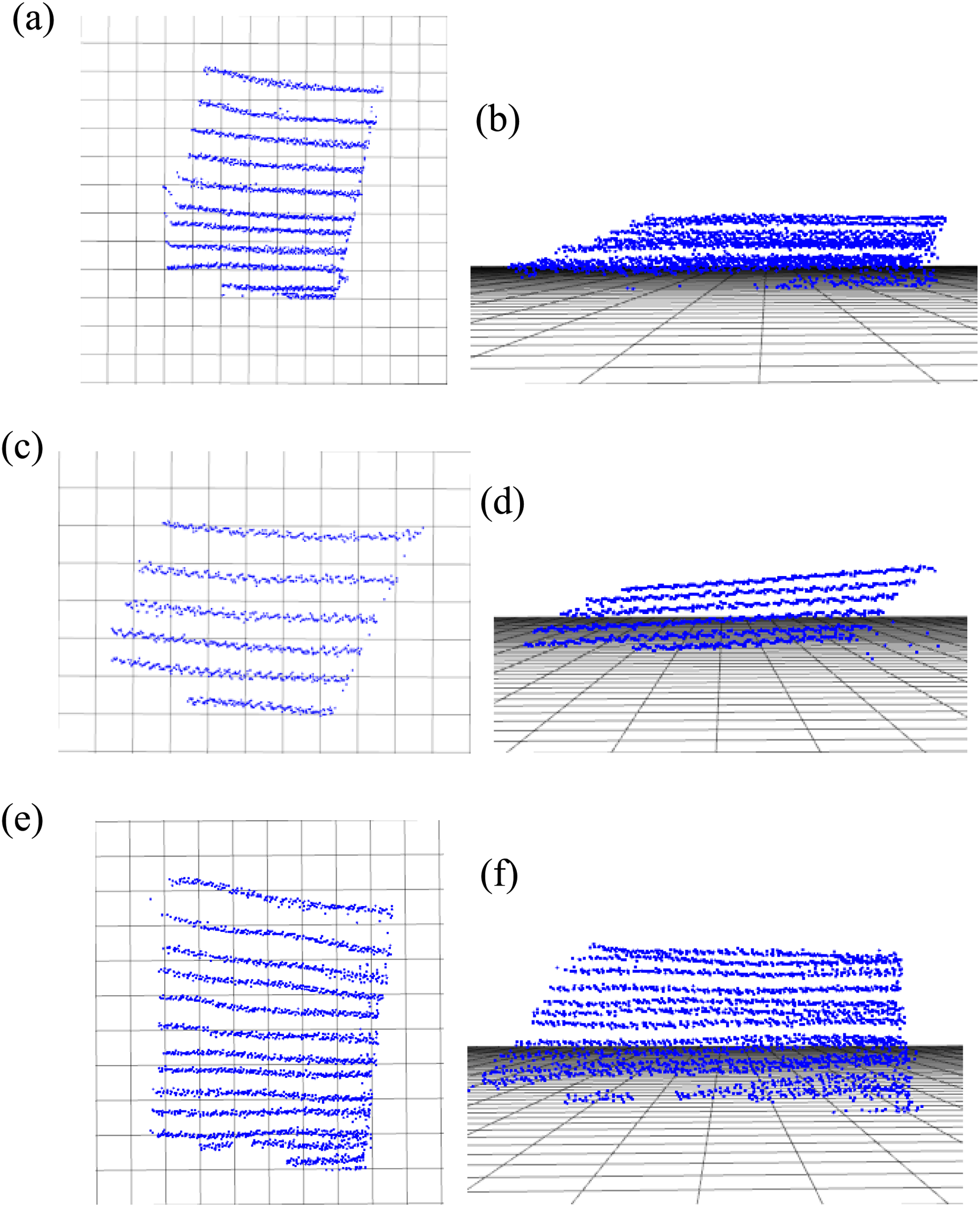
Point cloud of slopes A, B, and C. (a), (c), and (e) Top view; (b), (d), and (f) front view.

Figure 12(a) to (c) describes the estimation results with 50 times for slopes A to C, respectively. The results of our proposed method are depicted in red color, and the ground truth is expressed in blue color. It can be seen that compared with other methods, our method can achieve an accurate estimation for the slope angle. The statistic results of all methods are illustrated in Table 4, where the best results are demonstrated in red color. One can see that the proposed method is better than other methods in most cases.

Figure 12.

Accuracy comparison of different slope angle estimation methods. The estimation results of (a) slope A, (b) slope B, and (c) slope C.

Table 4.

Statistic results of slope angle estimation for different slopes.

Slope	Results	Ground truth	RANSAC	LMEDS	MSAC	RRANSAC	MLESAC	PROSAC	PCA	Least squares	Our method
A	Mean	7.74	8.102	8.155	8.163	8.154	8.275	8.040	8.494	8.467	8.018
	Variance		0.0437	0.0209	0.0562	0.0689	0.1212	0.0283	0.0080	0.0082	0.0145
B	Mean	13.86	14.26	14.25	14.25	14.26	14.22	14.24	15.02	14.92	14.23
	Variance		0.0979	0.0943	0.0984	0.0989	0.1827	0.0979	0.2345	0.2485	0.0915
C	Mean	18.51	18.56	18.54	18.55	18.54	18.56	18.57	18.77	18.74	18.53
	Variance		0.0254	0.0070	0.0183	0.0261	0.1944	0.0156	0.0057	0.0068	0.0053

RANSAC: random sample consensus, LMEDS: least median of squares, MSAC: m-estimator sample consensus, RRANSAC: randomized random sample consensus, MLESAC: maximum likelihood estimation sample consensus, PROSAC: progressive sample consensus, PCA: principal component analysis.

Robustness comparison

In this section, three objects with different sizes are placed on slope A, which are considered as three new slopes: A ₁, A ₂, and A ₃. These objects can be regarded as the interference to testify the robustness of the methods. The point cloud of slopes A ₁, A ₂, and A ₃ is shown in Figure 13.

Figure 13.

Point cloud of slopes A ₁, A ₂, and A ₃.

For slopes A ₁, A ₂, and A ₃, the estimation results with 50 times are given in Figure 14(a) to (c), respectively. The statistic results of all methods are illustrated in Table 5. Clearly, PCA and least squares methods are obviously affected by the interference. The larger the interference is, the worse the estimation result is. In contrast, the RANSAC family methods are less affected due to their characteristics where the outliers are removed.

Table 5.

Statistic results of slope angle estimation with different interferences.

Slope	Results	Ground truth	RANSAC	LMEDS	MSAC	RRANSAC	MLESAC	PROSAC	PCA	Least squares	Our method
A 1	Mean	7.74	7.904	8.024	7.952	7.908	8.120	7.946	8.643	8.601	7.854
	Variance		0.0714	0.0255	0.0668	0.0758	0.1366	0.1903	0.0204	0.0201	0.0097
A 2	Mean	7.74	7.950	8.021	7.972	7.960	8.238	7.929	8.502	8.470	7.862
	Variance		0.0491	0.0309	0.0472	0.0748	0.0649	0.0492	0.0186	0.0183	0.0125
A 3	Mean	7.74	8.099	8.077	8.090	8.259	8.072	8.179	8.737	8.707	8.026
	Variance		0.1328	0.0177	0.1341	0.4377	0.1767	0.1900	0.0047	0.0049	0.0168

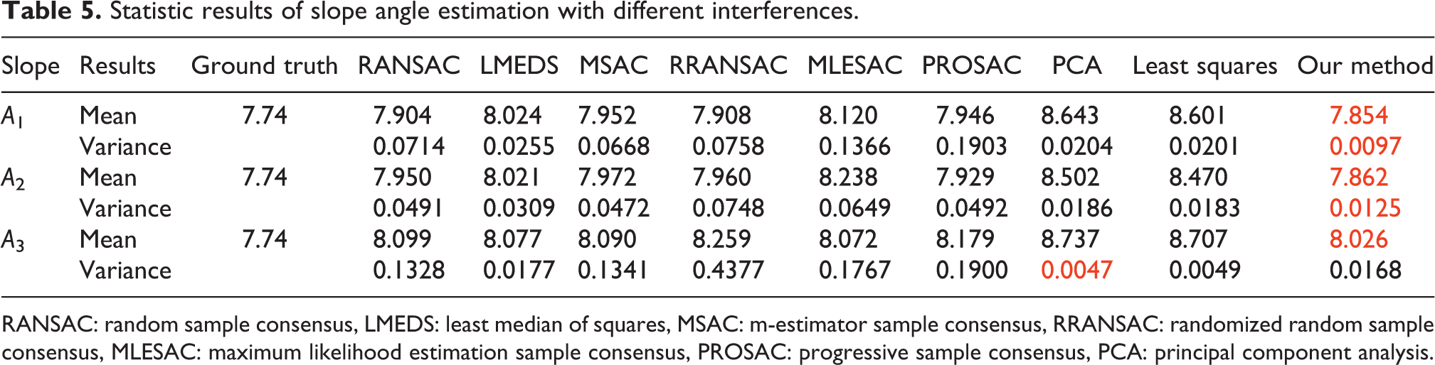
RANSAC: random sample consensus, LMEDS: least median of squares, MSAC: m-estimator sample consensus, RRANSAC: randomized random sample consensus, MLESAC: maximum likelihood estimation sample consensus, PROSAC: progressive sample consensus, PCA: principal component analysis.

Figure 14.

Robustness comparison of different estimation methods. The estimation results of (a) slope A ₁, (b) slope A ₂, and (c) slope A ₃.

Among these RANSAC family methods, the proposed method with the combination of RANSAC and least squares method is slightly superior to the others on the whole.

Conclusions

This article proposes a terrain description method for traversability analysis based on elevation grid map. Terrain features include height index, roughness, and slope angle. The proposed method can describe different types of terrain, including cluttered obstacles, potholes, and slopes. The experiments show that the measurements of obstacle’s height and pothole’s depth are effective. Real slopes can be distinguished with the help of roughness feature. The comparisons among different slope angle estimation methods are also conducted, which verify that the proposed method can achieve a better slope angle estimation.