Sage Journals: Discover world-class research

Abstract

Simultaneous localization and mapping (SLAM) plays an important role in fully autonomous systems when a GNSS (global navigation satellite system) is not available. Studies in both 2D indoor and 3D outdoor SLAM are based on the appearance of environments and utilize scan-matching methods to find rigid body transformation parameters between two consecutive scans. In this study, a fast and robust scan-matching method based on feature extraction is introduced. Since the method is based on the matching of certain geometric structures, like plane segments, the outliers and noise in the point cloud are considerably eliminated. Therefore, the proposed scan-matching algorithm is more robust than conventional methods. Besides, the registration time and the number of iterations are significantly reduced, since the number of matching points is efficiently decreased. As a scan-matching framework, an improved version of the normal distribution transform (NDT) is used. The probability density functions (PDFs) of the reference scan are generated as in the traditional NDT, and the feature extraction - based on stochastic plane detection - is applied to the only input scan. By using experimental dataset belongs to an outdoor environment like a university campus, we obtained satisfactory performance results. Moreover, the feature extraction part of the algorithm is considered as a special sampling strategy for scan-matching and compared to other sampling strategies, such as random sampling and grid-based sampling, the latter of which is first used in the NDT. Thus, this study also shows the effect of the subsampling on the performance of the NDT.

Keywords

Feature Based Scan-Matching 3D Navigation ML-NDT

1. Introduction

Simultaneous localization and mapping (SLAM) is of a great importance for autonomous systems in an environment where a global navigation satellite system (GNSS) is not reachable. Depending on the mapping structure, SLAM methods are mainly divided into two parts, proposed for dense mapping and feature-based mapping respectively. For feature-based SLAM (Fb-SLAM), the theory is well developed and has been applied to the indoor 2D case successfully. In Fb-SLAM, the state vector - holding the robot pose and landmark positions - and the uncertainty covariance matrix are estimated with well-known probabilistic filtering methods, such as a Kalman filter (KF), an information filter (IF) or a particle filter (PF). The landmarks are generally considered as points in Euclidean space and can be either artificial objects, like reflectors, or features extracted from the sensor data. Since the artificial landmarks can only be used in already-known areas, the feature extraction methods have a vital importance for Fb-SLAM in unknown environments. Besides, there is an important limitation on landmark quantities, since the proposed methods depend on the inverse of a state covariance matrix. On the other hand, the other groups of SLAM methods dealing with dense information are mostly based on scan-matching. A scan-matching method yields the rigid transformation parameters of the vehicle movement from two consecutive laser scans. Next, these relative transformations generate a graphical network and the history of the vehicle poses is obtained by solving this network. The 3D scan data have large numbers of points to be matched; thus, to be able to reduce the size of the matched points, a sampling strategy or a feature extraction method is a necessity for online SLAM. In our previous studies, we proposed a scan-matching method based on a multi-layered normal distribution transform (ML-NDT) [1] and a feature extraction method for a scan-matching method [2].

For the dense data mapping, scan-matching or image registration is the essential part of SLAM methods. For this purpose, most of researchers prefer to use the iterative closest point (ICP) scan-matching method [3]. The conventional ICP method is based on the minimization of the sum of all point-to-point distances. There are also point-to-plane and plane-to-plane variants of ICP, so as to increase robustness of scan-matching. An important disadvantage of the ICP algorithm is that it requires a nearest neighbourhood searching (NNS) algorithm to find correspondences between two scans. In addition, the ICP does not release any surface structure information; therefore, it is sensitive to noise and outliers. Another issue regards data storage, especially for large maps, since the unprocessed 3D data have to be saved for each scan. A normal distributions transform (NDT) is proposed as an alternative to ICP for fast and accurate scan-matching [4].

The main operation in the NDT is that the reference scan is divided into regular cells, and the surface is represented by the sum of normal probability density functions. Therefore, the map is represented in a much more compact form than the ICP. The input scan points are iteratively matched to the normal model of the reference scan by minimizing a Gaussian cost function with a Newton optimization method. This provides faster scan-matching and much less memory storage with respect to the ICP. NNS is not a problem at all for NDT, since there is no point-to-point distance measurement as in the ICP. On the other hand, the convergence time and the accuracy of the NDT-based scan registration are strongly related to the cell size. While the convergence time is small for very large cells, the convergence area is large. Therefore, the method generally results in incorrect parameter estimations. By way of contrast, for very small cell sizes the convergence time is high, but the accuracy is better if small transformations exist or else if the initial guess is insufficient. In the literature, there is no study offering a way of choosing the optimum cell size.

There are also some SLAM methods that extract features for scan registration purposes. They have significant advantages over a pure scan-matching method. The obvious advantage from the scan-matching point of view is that they are more robust than conventional methods. The reason is that the objects with certain geometric shapes - like lines or planes - are matched and irregular points - like bushes and tree leaves - are filtered out in the registration process. Another advantage is that the method does not need high precision odometry data since scan-matching is based on the features. In addition, a fundamental problem in scan-matching is that the loop detection problem and can be solved easily if the features of the environment are available. These properties are significant for 3D outdoor and large-scale SLAM since the environment is complex and includes noise and outliers.

In this paper, we propose a fast and robust scan registration method using feature points extracted from the input scan for 3D outdoor SLAM. The method consists of two main parts, namely feature extraction and scan-matching. In feature extraction, a probabilistic plane extraction procedure is applied via a RANSAC algorithm to the discretized point cloud. As a scan-matching method, an improved version of the NDT, called ‘multi-layered NDT’ (ML-NDT) is used. This method computes the cell sizes automatically from the point cloud boundaries in a structured manner. In the generative phase of the algorithm, the probability density functions (PDFs) of each scan in all the layers are computed for the reference scan. For the input scan, which is the one to be registered to the reference scan, the plane inliers are extracted with the stochastic plane detection method. In the matching process, instead of using the all the scan points (or sampled points) as with standard NDT and ML-NDT, these inlier points are used. In this way, the feature-based ML-NDT (FbML-NDT) algorithm possesses several advantages. The first is that the registration processing time - which is the most time consuming part of scan-matching algorithms - is significantly reduced. The scan-matching method is more robust than the conventional methods since the matching is based on plane structures. In this study, we also investigate the effect of sampling strategies - like random sampling and grid-based sampling - on the performance of the ML-NDT method, and the proposed feature extraction method is compared to these subsampling methods. The proposed method does not directly solve the SLAM problem since it is a registration method. The SLAM methods proposed by [5] or [6] can be used for this purpose.

In the next section, we give a summary of related works in the area of scan-matching-based SLAM. In Section 3, we introduce the feature extraction and ML-NDT scan-matching methods and combine them into a single framework for robust and fast scan-matching. The experimental results are given in Section 4 and conclusions are drawn in Section 5.

2. Related Works

In this section, the scan-matching-based SLAM methods are explained. In addition, the sampling strategies and feature extraction for scan-matching algorithms are investigated.

2.1 Scan-matching Methods for SLAM

The iterative closest point algorithm (ICP) is a well-known method for 3D scan-matching [3]. Recently, Ohno proposed a modified ICP method for real-time 3D map-building by using a 3D camera [6]. A network-based solution - called ‘globally consistent range scan alignment’ - and its application to 3D SLAM is introduced in [7]. In order to increase the robustness of the ICP method, variants of ICP matching techniques have been proposed, such as point-to-plane [8] and plane-to-plane matching techniques [9]. Also, in [9], a generalized ICP framework is proposed, combining the already-mentioned ICP algorithms into a single probabilistic structure. Since the conventional ICP is based on the point-to-point sum of distance minimization problem, it requires a high computation time on a nearest neighbourhood search (NNS) to find corresponding points. For a typical ICP, NNS takes O(MN) computation time. This time can be reduced by up to O(Nlog(M)) by using the kd-tree space quantization method [10]. In addition, the original ICP does not release any surface structure information; therefore, it is quite sensitive to noise and outliers. The data storage is another issue for the ICP method, especially for large maps, since the unprocessed 3D data has to be saved for each scan. For long-range and outdoor SLAM, a novel scan-matching method - NDT - is proposed as an alternative to ICP.

NDT was first applied to the 2D case by Biber and Strasser [4]. Later, it was extended to the 3D case by Takeuchi and Tsubouchi [11]. A marker-free registration was adapted to a 3D laser scan by dividing the point cloud into multiple slices and applying a 2D NDT algorithm [12]. They proposed three modifications on the original NDT: a coarse-to-fine strategy, multiple slices and the Levenberg-Marquardt algorithm as the optimization method. In [11], an improved 3D NDT for 3D scan-matching was proposed. The main contribution of this study is to modify the 2D NDT to a 3D NDT. The method uses different cell sizes for dual resolution to accelerate the method. It starts with a large cell size and, after the convergence of the score function, they use small cell sizes. A recent study based on 3D NDT was introduced by Magnusson. He uses 3D NDT for scan registration for autonomous mining vehicles [13] and the loop detection problem in SLAM [14]. A different convergence calculation method of the NDT-based high resolution grid map for 2D NDT was introduced in [15]. They used small cell sizes for high resolution grid map representation and applied eigenvalue expansion to speed up the convergence time. They also used similar representation for sub-grid object recognition [16].

The authors proposed a ML-NDT structure computing the cell sizes in each layer automatically from the point cloud boundaries instead of using a fixed cell size [1]. Also, the cost function is described as a Mahalanobis distance function, and Levenberg-Marquardt and Newton optimization methods are adapted to the method. In this way, the convergence rate and the estimation of the amount of relative transformation is improved. An application of the conventional NDT scan-matching to the SLAM problem using an EKF filter was recently introduced in [17] for the 2D case. In [5], a combination of ML-NDT with a Kalman filter for a 3D SLAM problem is presented. In the paper, the 6D localization of the mobile robot is obtained with the help of low quality 2D odometry data. In general, the scan-matching methods suffer from the computational cost of the matching process due to iterative optimization methods. Mostly, the scan to be registered is sampled randomly; however, this is not an optimum means since the point cloud does not have a uniform distribution. To overcome this issue, other sampling methods described in [18], which is applied to ICP, are discussed in the next subsection.

2.2 Sampling Strategies for Scan-matching

A common bottleneck of current scan-matching methods is the numbers of points matched in the registration process. Even if we consider a simple scan, there are more than 10,000 points. Therefore, the selection of a subset from the point cloud is a critical issue for a fast and accurate algorithm. In the literature, there are some well-known sampling strategies implemented with ICP [18] for 2D point clouds, and generally they can be categorized as follows;

Always using all the points.

Uniform subsampling.

Random subsampling in each iteration.

Selection of points with a high intensity gradient.

Selection of points from one scan or both scans.

Selecting points such that the distribution of normals among the selected points is as large as possible.

From the NDT point of view, if the all methods are considered, we can say that the first method is not suitable for two reasons. The obvious one is that the number of points to be matched is very high; therefore, convergence may take a very long time. The second reason is that the point cloud might be very noisy or unstructured due to the nature of the environment. Therefore, a sampling strategy must be carried out. The second sampling strategy, which is uniform subsampling, also may not be suitable if the point cloud is not uniformly distributed, which is generally encountered in 3D outdoor scanning due to the hardware configuration. Random subsampling, the third strategy, seems reasonable, but again due to non-uniform distribution the dense regions have more weights than the sparse regions. Since we do not have any intensity information in LiDAR-only systems, the fourth strategy - the selection of points with a high intensity gradient - cannot be considered. The fifth method - the selection of points from both scans - can be applied; in addition, since the point cloud is represented by the sum of Gaussians, in the NDT generative process, the sampling should be dense enough for good modelling. For this reason, we recommend very dense sampling for the reference scan. Finally, the last strategy is also meaningful for the input scan; however, finding the large normal distribution for selected points requires significant computation time due to NNS. Moreover, and for the outdoor case, the outliers should be taken into consideration.

2.3 Feature-based Scan-matching in SLAM

None of the just mentioned sampling strategies take the geometric or characteristic information into account when selecting the sample points. For this reason, instead of sampling randomly, the feature points are extracted from the point clouds and used in the matching process. Thus, the registration time is reduced effectively and efficiently. An important advantage of some feature-based scan-matching algorithms is that they can work without any initial parameter estimation, which is mostly provided by an odometer [19]. A line feature-based scan-matching method for 2D SLAM is proposed in [20]. For another 2D indoor case, a navigation method depending on combined feature-based scan-matching and FastSLAM is proposed in [21]. They used line segments and their properties - like slope and end points - as features. They used a FastSLAM algorithm for filtering purposes. Their feature extraction algorithm uses a global filtering method that utilizes a line fitting algorithm and a split-and-merge method. Recently, Pathak proposed a plane-feature based scan-matching algorithm for the 3D case [22]. As with 2D implementations, instead of detecting line segments, plane segments are extracted from the 3D point cloud and then matched to find rigid body transformation parameters. In their another study, they use extracted planar features for online 3D SLAM and make a detailed performance comparison between their method and ICP [23]. In their work, the pose-graph relaxation is used as a SLAM method instead of conventional probabilistic SLAM, since planar features can only be used for registration purposes. The projection and convex-hull computations of the planar features are necessary to represent a plane in a finite region. Point cloud data provided in 3D can be processed by converting it to a 2D range image to extract the feature points for scan-matching purposes. Sehgal et al. propose an approach enabling SIFT application to locate scale and rotation invariant features in 3D point clouds [24]. The algorithm, running on a real-time system, uses these features in ICP scan registration. An interesting study using the soft computing method - growing neural gas (GNG) - to generate 3D models is introduced by Viejo et al. [25]. They used the GNG structure to compute planar patches and robot positions by applying a 3D model registration algorithm.

This study is different than the above-mentioned methods in three ways. Firstly, the conventional or feature-based scan-matching methods use the ICP algorithm; in contrast, the proposed scan-matching method using feature points uses an improved NDT algorithm. A detailed comparison of the NDT and ICP methods is given by Magnusson [26]. Although the ICP methods are solely dedicated to scan-matching, the NDT and its variants cannot be considered as just a scan-matching method. Since NDT provides the surface representation of the point cloud - like smoothness and orientation - it can also be used as an efficient surface analysis and loop detection method in addition to registration [14]. Secondly, the feature extraction method based on statistical plane detection is easy to implement, robust and fast. In addition, it can be modified to an EKF-based 3D SLAM-structured environment reconstruction method [27]. Thirdly, the effect of subsampling methods on the performance of NDT and its variants is never considered, although it is investigated for the ICP. Besides these considerations, the proposed feature extraction method is considered as a special sampling strategy and compared with the introduced subsampling methods.

3. A Fast and Robust Feature-Based Scan-Matching Method

In this section, the details of the feature based scan-matching method are explained. Firstly, the scan-matching, ML-NDT and plane detection methods are explained in turn. Next, using the extracted plane inlier points in the registration process of the ML-NDT algorithm, a feature-based scan-matching method is obtained. Secondly, the grid-based sampling strategy is proposed for the ML-NDT method and a comparison among the feature-based, grid-based and regular sampling methods is discussed.

3.1 Multi-layered Normal Distribution Transform (ML-NDT)

The convergence time and accuracy of the NDT-based scan registration methods are highly correlated with the cell size. While the convergence time is small for large cells, the convergence area is large; therefore, the system mostly results in incorrect parameter estimations. On the other hand, for small cell sizes the convergence time is high, but the accuracy is better if small transformations exist or the initial transformation parameters are sufficient. In the literature, there is no study offering a way for choosing the optimum cell size. The authors proposed a ML-NDT structure that computes cell sizes in each layer automatically from the point cloud boundaries instead of using a fixed cell size [1]. In the study, the cost function is described as a Mahalanobis distance function, and Levenberg-Marquardt and Newton optimization methods are adapted to the presented method. In this way, the convergence rate and the estimation of the amount of transformation parameters are improved. In [5], a combination of a ML-NDT with a Kalman Filter for 3D SLAM implementation is proposed.

An NDT is described as a set of PDFs. The first step in NDT is to divide the point cloud into regular cells. Next, for each cell, the mean and covariance values are calculated and stored. If the first and second moments of the discretized reference scan are computed by a D-dimensional normal random process, then the probability density of a chosen point, x, is computed as:

p (x) = \frac{1}{{(2 π)}^{D / 2} \sqrt{| C |}} e^{- \frac{{(x - μ)}^{T} C^{- 1} (x - μ)}{2}}

(1)

where μ and C represent the mean vector and covariance matrix of the reference scan points within the cell including the point x. Each PDF can be considered as an approximation of the local surface describing the position of the surface with its orientation and smoothness. The surface orientation and smoothness are determined by the eigenvectors and eigenvalues of the covariance matrix. Depending on the eigenvalues and eigenvectors, the distribution can be a point, a line, an ellipsoid or circle-shaped in 2D. In 3D, if two eigenvalues are equal and the one eigenvalue is too small with respect to the others, the point cloud distribution denotes a plane. With the similar idea, it is possible to represent other important geometric surfaces, like a sphere and a 3D ellipsoid, by an NDT [14].

The mean (μ) and covariance (C) of each cell is defined as follows:

μ_{i} = \frac{1}{N} \sum_{j = 1}^{N} B_{i j}

(2)

C_{i} = \frac{1}{N - 1} \sum_{j = 1}^{N} (B_{i j} - μ_{i}) {(B_{i j} - μ_{i})}^{T}

(3)

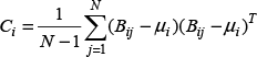
where i represents the cell index and j represents the point index in each cell. N denotes the number of points in a cell and B_ij collects all 3D point positions contained in the cell (box). Thus, each cell has PDFs describing the point cloud in a piecewise smooth representation with continuous derivatives.

ML-NDT uses a multi-layered structure dividing the point cloud into qⁿ regular cells in each layer. Here, n stands for the layer level and q is the division parameter. The greater the value of n, the more frequently that the small-sized cells are obtained. For the 2D case, q is chosen as four while it is chosen as eight for 3D. In Figure 1, the point cloud and its second layer normal distribution are shown. The point cloud taken from the experimental Navlab SLAMMOT dataset has 361 points [28]. The point cloud is first divided into 16 regular cells, and the cell boundaries are shown with white edges for illustration. The brighter points indicate a higher probability, and this representation also corresponds to the second-layer normal distribution transform of the multi-layered representation. In Figure 2, the multi-layered representation of the same point cloud given in Figure 1 is shown. In each layer, i, the point cloud, is subdivided into 4ⁱ equal parts, where i=1,2,3. The cell boundaries are plotted only for occupied cells. The second-layer surface representation of the given point cloud based on a normal probability function is shown in Figure 3.

Figure 1.

Second-layer ML-NDT representation. The red spots show the point cloud

Figure 2.

The point cloud and its first-, second- and third-layer NDT representations

Figure 3.

Surface representation of the point cloud given in Figure 1

The vital part of the NDT method is the discretization process of the point clouds. These discretization artefacts coming from the subdivision process leads to discontinuities in the surface representation and can be problematic in some cases. There are two possible reasons that cause discretization errors. The first one is the selection of the cell size that describes the resolution. The lower the cell size, the smaller the modelling error that is obtained. Therefore, the small sizes should be selected so as to minimize this kind of discretization or modelling error. An example of this type of error is seen in Figure 2 in the cell centred in (300,-200). The model in this cell contains considerable errors, since it does not represent the actual distribution. If the cell sizes are reduced, this error is broadly eliminated. Another discretization error occurs at the borders of the cells. Therefore, it is possible to encounter a PDF for a cell that is non-zero, even at points outside the borders of cells, as seen in the cell centred in (100,200) in Figure 2. In the conventional 2D NDT implementation, this type of discretization effect is minimized by using four overlapping 2D cell grids with bilinear interpolation [4]. A similar approach is also used by Magnusson in 3D NDT by using eight regular 3D cells with trilinear interpolation [26]. It is seen that this kind of interpolation increases the computation by at most eight times.

For the 3D case, the point cloud obtained from the Hannover dataset [29] and its fourth-layer NDT representation is given in Figure 4. The ellipsoids are drawn by using the mean vector and covariance matrix of the occupied cells. If the number of points is less than a threshold value, this cell is ignored.

Figure 4.

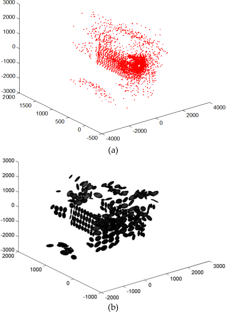
(a) A point cloud in the Hannover campus dataset; (b) The fourth-layer NDT representation

After the point cloud is represented by a multi-layered structure, the iterative Newton optimization method is applied. The ML-NDT algorithm given in Table 1 allows for two different optimization methods, such as Newton or Levenberg-Marquardt. Here, we only express the Newton-based optimization. The aim of the algorithm is to obtain relative transformation parameters from two successive scans. The ML-NDT algorithm and its steps, which are a splitting process, a generative process and a registration process, are given in Table 1. Before the splitting process, a layer number must be defined. Next, the point cloud limits are calculated and the left-down and up-right corners of each cell in all the layers are computed. In the splitting process for all the layers, the point cloud is distributed to equally-sized cells.

Table 1.

ML-NDT Algorithm

Algorithm (ξ) = ML - NDT (R,S,q,n,s)

Inputs:

R: Reference scan

S: Subsampled scan

q: Division constant

n: Number of layers

s: Starting layer

Outputs:

ξ: Relative transformation parameters (translations and rotations)

Splitting Process

1: for all layers l_i (i=1,2,‥n) do

2: Divide the point cloud into qⁱ cells

3: for all ri ∊ R do (ri is the i^th point)

4: Find the cell cj that includes ri, then store ri in cj

5: end for

6: end for

Generative Process

1: for all layers li (i=1,2,‥n) do

2: for all cells cj ∊ C do

3: if number of points in cj > 4

4: Calculate the covariance and mean values of each cell cj and store to B

5: end if

6: end for

7: end for

Registration Process

1: Start with the layer s

2: Wait for the convergence

3: for each point in si ∊ S do (si is the i^th point)

4: find the corresponding cell in the reference model B

5: Update ∊ by following equations (4) through (12)

6: Switch to the next layer in every three iterations.

7: end for

8: return ∊

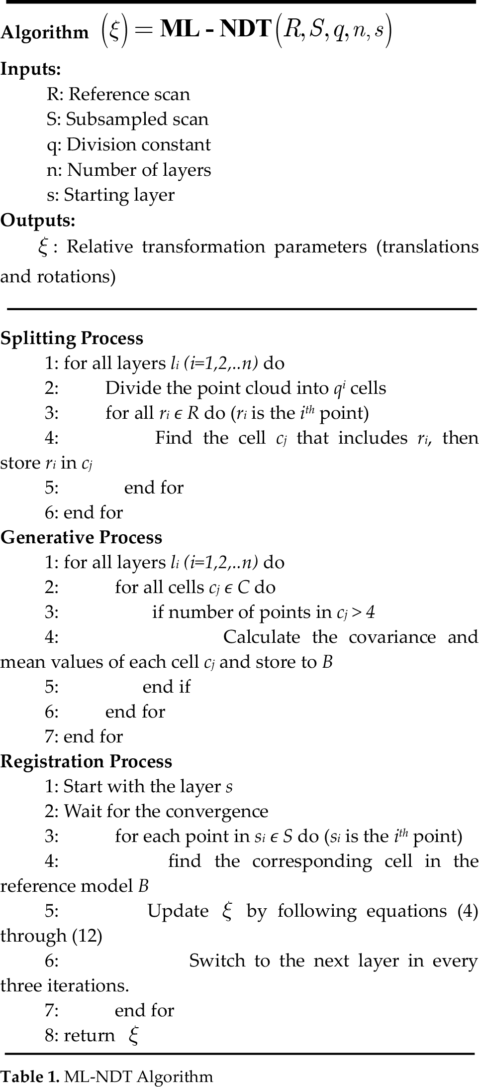
In the generative process, for all layers and each cell, covariance matrices and mean vectors are calculated and stored to the B cell array if a cell contains more than four points. Thus, the point cloud is represented as a sum of piecewise Gaussian probability density functions.

Finally, in the registration process, a starting layer s is defined based on the quality of the odometry data. First, a switching criteria based on the variation of the score function is searched; however, it is observed that the score function variation does not always decrease monotonically. Therefore, it is not plausible to propose switching criteria based on the score function; therefore, for the sake of simplicity, each layer runs three times, except for the last layer. Since this switching mechanism does not depend on the score function, the information flow between the layers is isolated. The only information shared by the layers is the point cloud, and there is no direct relation among the layers since they are constructed from the point cloud directly. In the last layer, where it has the highest resolution, the algorithm runs until the convergence criteria are met. The convergence criteria depend on two factors, namely the norms of the number of parameter updates and the number of iterations. Here, S represents the subsampled points from the input scan. In practice, 10-20% of the input scan is sufficient for successful convergence. The issue of choosing subsamples is discussed in Section 2.3.

The transformed point is denoted as x', given by (4), while R represents the rotation matrix containing the Euler angles (α,β,γ) in (5). The translation vector, t, is given by (6):

x' = R x + t

(4)

R = [\begin{matrix} 1 & 0 & 0 \\ 0 & c α & - s α \\ 0 & s α & c α \end{matrix}] [\begin{matrix} c β & 0 & s β \\ 0 & 1 & 0 \\ - s β & 0 & 0 \end{matrix}] [\begin{matrix} c γ & - s γ & 0 \\ s γ & c γ & 0 \\ 0 & 0 & 1 \end{matrix}]

(5)

t = [\begin{matrix} t_{x} \\ t_{y} \\ t_{z} \end{matrix}]

(6)

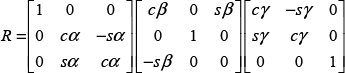
where x = (x,y,z) is an input scan point and x' is the transformed point based on the initial parameters provided by the odometry. The initial values of the rotations and translations are accepted as zero if there is no odometry or IMU sensor information. In fact, all the scan-matching algorithms - ICP, NDT and ML-NDT -require these initial values. However, we observed that in some cases the ML-NDT converges on the correct transformation parameters without any initial parameters.

Let e be the error vector between the transformed point and the mean of the corresponding cell. Based on this error e and the covariance C of this cell, the Mahalanobis distance score function is defined as follows:

e = x' - μ_{i}

(7)

S c o r e = \sum_{k = 1}^{M} e^{T} C^{- 1} e

(8)

Another important issue is to get rid of singularities on the covariance matrix, C. The computation of the score function (8) requires the inverse of C. The matrix C may easily become singular just in case the point distribution in a cell is perfectly collinear or coplanar. A solution is proposed by Magnusson, who slightly inflated the covariance matrix C whenever it was found to be nearly singular [14]. If the largest eigenvalue l₃ of C is more than 100 times greater than l_j where j=1,2 represents the other eigenvalue indices, then the eigenvalues are replaced with l_j'; = l₃/100. The new covariance matrix is replaced with C’ = V Λ‘V, where V contains the eigenvectors of C and Λ’ = diag(l₁‘, l₂’,l₃).

The rigid body transformation parameters are collected in a vector as given in (9), and they are estimated iteratively by using the Newton method:

ξ = {[t_{x} t_{y} t_{z} α β γ]}^{T}

(9)

To be able to minimize the score function with respect to the transformation parameters, ξ, the gradient vector, g_k, and the Hessian matrix, H_k, of the summand of the score function, such that S_k can be written as follows:

s_{k} = e^{T} C^{- 1} e

(10)

g_{k} = \frac{\partial s_{k}}{\partial ξ} = \frac{\partial s_{k}}{\partial e} \frac{\partial e}{\partial ξ} = e^{T} C^{- 1} \frac{\partial e}{\partial ξ}

(11)

H_{k} = \frac{\partial^{2} s_{k}}{\partial ξ_{i} \partial ξ_{j}} = {(\frac{\partial e}{\partial ξ_{j}})}^{T} C^{- 1} \frac{\partial e}{\partial ξ_{i}} + e^{T} C^{- 1} \frac{\partial^{2} e}{\partial ξ_{i} \partial ξ_{j}}

(12)

For derivations of $\frac{\partial e}{\partial ξ_{i}}$ and $\frac{\partial^{2} e}{\partial ξ_{i} \partial ξ_{j}}$ , one can look at [14]. The transformation parameters, ξ_t, are updated iteratively as follows;

ξ_{t} = ξ_{t - 1} - H^{- 1} g

(13)

where g and H are computed as follows:

g = \sum_{k = 1}^{M} g_{k}

(14)

H = \sum_{k = 1}^{M} H_{k}

(15)

In the next section, the grid-based sampling strategy is explained.

3.2 Grid-based Sampling for ML-NDT

A sampling strategy called ‘grid-based sampling (GBS), for any scan-matching algorithm, and especially for ML-NDT, is proposed. GBS sampling is applied to an input scan by two steps. First, the point cloud is divided into fixed cells, while in the second step, an equal number of samples is selected from each cell if the number of points is greater than a threshold value. In Figure 5, the difference between the regular sampling and the grid-based sampling is shown. As we can see, the distribution of the sampled point clouds looks very different even though the selected number of points is the same. The GBS point cloud is more homogenous than the regular or random sampled point cloud.

Figure 5.

(a) The effect of the GBS sampling strategy. The original point cloud taken from Ford data set [30] is subsampled regularly. (b) The GBS is applied to same point cloud. Each figure has an equal number of points and is top-viewed

3.3 Feature Extraction

In this section, the steps of the 3D robust feature extraction algorithm are explained. The method starts with point cloud discretization by dividing the point cloud into regular cells and assigning each point into these cells. This step is also known as the splitting or discretization process. The well-known and simple discretization method is to use fixed cells; however, there are other methods, such as tree representations, iterative discretization and adaptive clustering [14]. In this study, the size of a cell is calculated from the point cloud boundaries by dividing the point cloud volume into 8₄ (4,096) equal-volume cells, where this division number originated from the Octree representation and corresponds to the fourth-layer of ML-NDT splitting process.

After the discretization process, planar segments are detected by first finding the inliers of a plane via the RANSAC algorithm [31]. Next, if the number of inlier points in a cell exceeds a threshold value (in practice, 10), the least mean square plane fitting is applied to these inliers to obtain the parametric representation of the plane.

A Hessian normal form of a plane can be written as follows:

β_{a} x + β_{b} y + β_{c} z + β_{d} = 0

(16)

where the vector β represents the infinite plane parameters. Wherever the first three elements of the vector β denote the normal vector (n), the distance to the origin is represented by the last element of β. The constraint matrix is constructed as follows:

A = [Γ_{x} Γ_{y} Γ_{z} 1]

(17)

where Γ indicates the columns of the plane points given in the x, y and z axes. The last column of the constraint matrix A is filled by ones, and then singular value decomposition (SVD) is applied to A, as in (18). The last column of the eigenvector matrix V ∊ R³ yields the plane parameters as the vector β (19):

A = U E V^{T}

(18)

β = V_{j 4} (j = 1, 2, 3)

(19)

If there are large point sets and the outliers exist, this method becomes defective in terms of its computational burden and accuracy. Instead, principal component analysis (PCA) can be used. The covariance matrix of all the points belonging to the plane is found. Next, SVD is applied to the covariance matrix. The last column corresponding to the smallest variation axis gives the normal vector of the plane. The parameter β_d is found by placing any plane point into (16).

The extracted plane points from the point cloud provided by the Hannover dataset are shown in Figure 6. The size of the points to be matched is almost 10% of the original point cloud. In the next section, the FbML-NDT algorithm using the extracted plane inlier points in the matching process is explained in detail.

Figure 6.

Feature points extracted from the point cloud

3.4 Feature-based Multi-layered Normal Distribution Transform (FbML-NDT)

In this part, a novel scan-matching method using an ML-NDT algorithm based on extracted features is introduced. For the reference scan, the regular ML-NDT is applied to each layer, while for the input scan - which is that to be aligned to the reference scan - the plane inliers are extracted as explained in the previous section. Next, for each plane point, the regular registration process is applied as given in Section 3.1.

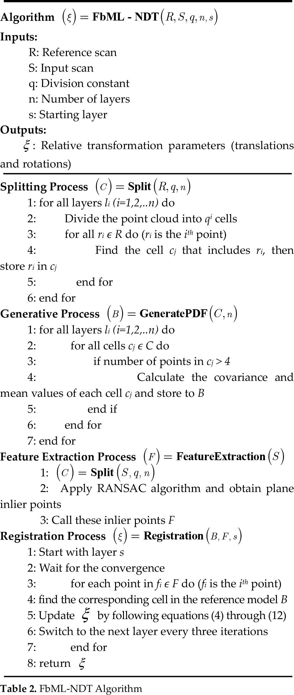
The algorithm of the FbML-NDT is given in Table 2. It consists of four phases, namely a splitting process, a generative process, feature extraction and a registration process. In the splitting process, the reference scan is divided into fixed cells, while in the generative process the mean vector and the covariance matrices of each cell are computed as in ML-NDT. In the feature extraction process, the input scan is also discretized and the plane candidates are detected via the RANSAC algorithm. If the number of inliers in a plane is greater than a threshold value, then these plane inlier points are considered as feature points (F) for the registration process. In the registration process, the extracted feature points are used in the optimization step of the ML-NDT algorithm; thus, the number of matching points is reduced effectively and efficiently. The rigid body transformation parameters, ξ, are obtained as a result of the algorithm.

Table 2.

FbML-NDT Algorithm

Algorithm (ξ) = FbML - NDT(R,S,q,n,s)

Inputs:

R: Reference scan

S: Input scan

q: Division constant

n: Number of layers

s: Starting layer

Outputs:

ξ: Relative transformation parameters (translations and rotations)

Splitting Process (C) = Split(R,q,n)

1: for all layers l_i (i=1,2,‥n) do

2: Divide the point cloud into qⁱ cells

3: for all ri ∊ R do (ri is the i^th point)

4: Find the cell cj that includes ri, then store ri in cj

5: end for

6: end for

Generative Process (B) = GeneratePDF(C,n)

1: for all layers li (i=1,2,‥n) do

2: for all cells cj ∊ C do

3: if number of points in cj > 4

4: Calculate the covariance and mean values of each cell cj and store to B

5: end if

6: end for

7: end for

Feature Extraction Process (F) = FeatureExtraction(S)

1: (C) = Split (S,q,n)

2: Apply RANSAC algorithm and obtain plane inlier points

3: Call these inlier points F

Registration Process (ξ) = Registration(B,F,s)

1: Start with layer s

2: Wait for the convergence

3: for each point in fi ∊ F do (fi is the i^th point)

4: find the corresponding cell in the reference model B

5: Update ξ by following equations (4) through (12)

6: Switch to the next layer every three iterations

7: end for

8: return ξ

The feature extraction for scan-matching can be considered as a special case of the subsampling method. This is true in terms of point reduction in the registration process of the scan-matching method. However, since the feature extraction-based scan-matching utilizes the geometric structures - which are planes in this paper - they are more robust than the conventional methods, even if they are sampled with the GBS strategy. Another issue is that the GBS method samples an equal number of points from all the cells and does not take the importance of a cell into account. In the next section, the performance analysis of the feature-based scan-matching and the effect of sampling strategies is given.

4. Performance Analysis and Experimental Results

This section includes the performance analysis of the proposed method and the experimental results. Two different datasets - the Ford dataset [30] and the Hannover dataset [29] - are used for this purpose. This section is mainly divided into two parts. In the first part, an analysis of the feature-based scan-matching algorithm and the performance of the parameter update step are given. In the second part, the feature extraction method is considered as a special case of a sampling strategy and compared to other sampling strategies, namely regular sampling, random sampling and the GBS introduced in this study.

4.1 Performance of the FbML-NDT

To show the convergence speed of the FbML-NDT algorithm without any initial transformation, the parameter update steps are shown in Figure 7. With this registration, the ground truth transformation obtained by GPS and an Applanix POS LV sensor is known as two meters in the y direction. In this path, the laser scanner collected five scans, and each scan was obtained at approximately 0.4 meter intervals. These scans are indexed as the 1000^th-1004^th scans in dataset [30]. It was observed that the algorithm successfully estimated the correct transformation within a few centimetres' error in three iterations. In this registration, no initial transformation parameters were used as with odometry, and they are assumed to be zero. However, the algorithm may fail if long range transformations exist. Therefore, the odometry data for initialization improves the system's robustness and speed.

Figure 7.

Parameter update. From the ground truth data, obtained via GPS and an Applanix POS-LV sensor, the vehicle moved two meters in the y direction and there was no change in other directions and orientations (degree)

More comprehensive results showing the performance of the feature-based scan-matching method are given with the comparisons of the sampling strategies in the next subsection.

4.2 Comparisons of Sampling Strategies with Feature Extraction

As a further analysis, the feature extraction method is considered as a special sampling method, and its performance is compared with the sampling strategies described in Section 3.2. For this analysis, the Hannover dataset is used and the odometry data given by it is in two dimensions with three parameters, namely, the translation in the x-z axes and the rotation (θ) about the y axis. The odometry error variation with respect to the ground truth is shown in Figure 8. In our representations, the heading angle corresponds to β and all the error variations are given with respect to the ground truth data provided by the dataset.

Figure 8.

The odometry error variation for the first 100 scans in the Hannover 1 dataset [29]: (a) Relative translation error variation; (b) Relative rotation error variation

The scan-matching rotation and translation error variations of the FbML-NDT algorithm are given in Figure 9. The odometry data is used as an initial point for all sampling strategies. As can be seen, the mean of the translation and rotation error is very close to zero and the performance is much better than the odometry. It is also possible to say that the measurement error can be considered as the zero mean Gaussian distribution.

Figure 9.

(a) FbML-NDT relative translation error variation; (b) Relative rotation error variation

Comparisons of all the sampling strategies with respect to their translation and rotation angle errors are given in Figure 10. As seen from the charts, the performance of the proposed sampling strategies - GBS and FBS - provides satisfactory results. The mean of the translation error is less than 2 cm and that of the rotation error is less than 0.3 degrees, while the translation error is about 50 cm in the case of odometry and about 7 cm in that of random sampling. The standard deviations of the combined translation errors are almost the same at around 30 cm, while the standard deviations of the combined rotation errors are around 1 degree. Furthermore, the error variation can be modelled as a normal distribution since it is not biased as in the case of the odometry error. Therefore, Gaussian filters such as Kalman and information filters can be successfully used with the proposed method since they are optimum under Gaussian noise.

Figure 10.

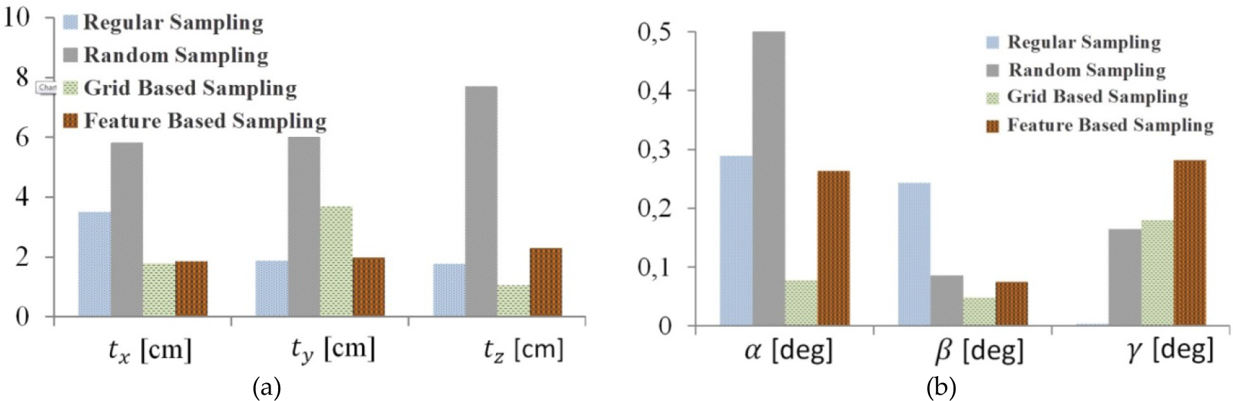
Performance comparisons of all the sampling strategies: (a) Average translation errors; (b) Average rotation errors

A more important aspect of the comparisons of the methods is given in Table 3. The methods are compared with their other properties out of 100 scans, such as the average iteration number, the percentage of matched points, the convergence time and the success rate.

Table 3.

Performance comparison of the sampling strategies

	Num. of iteration	Matched points (%)	Matching time (sec)	Success Rate (%)
Regular Sampling	17.27	12.17	44.701	97
Random Sampling	17.24	12.16	43.84	97
Grid-based Sampling	14.29	9.16	7.4586	99
Feature-based Sampling	12.67	3.19	2.5087	100

With the success rate computations, it is assumed that the algorithm is successful if the translation errors are less than 200 cm and the rotational errors are less than 10 degrees, otherwise it is assumed that the algorithm diverges and is not dependable. As seen from the table, the success rate is 100% and the convergence time is about 2.5 seconds in MATLAB. These show that the proposed feature extraction method is more robust and faster than the other sampling strategies.

The FbML-NDT and odometry localization performances out of 100 scans are shown in Figure 11 (a). The error norm of the robot position with respect to the ground truth is shown in Figure 11 (b). While the odometry-based navigation is very poor due to biased error, the FbML-NDT-based navigation is fairly good. At the end of the path, the absolute error is more than 60 metres for odometry-based localization. On the other hand, this error is about 7 metres if FbML-NDT is used. Finally, a visual map, including planar feature points which is extracted from the point cloud, is given in Figure 12. Here, the feature points belonging to the ground planes are eliminated to make the figure clear. In addition, the robot positions are shown in Figure 12.

Figure 11.

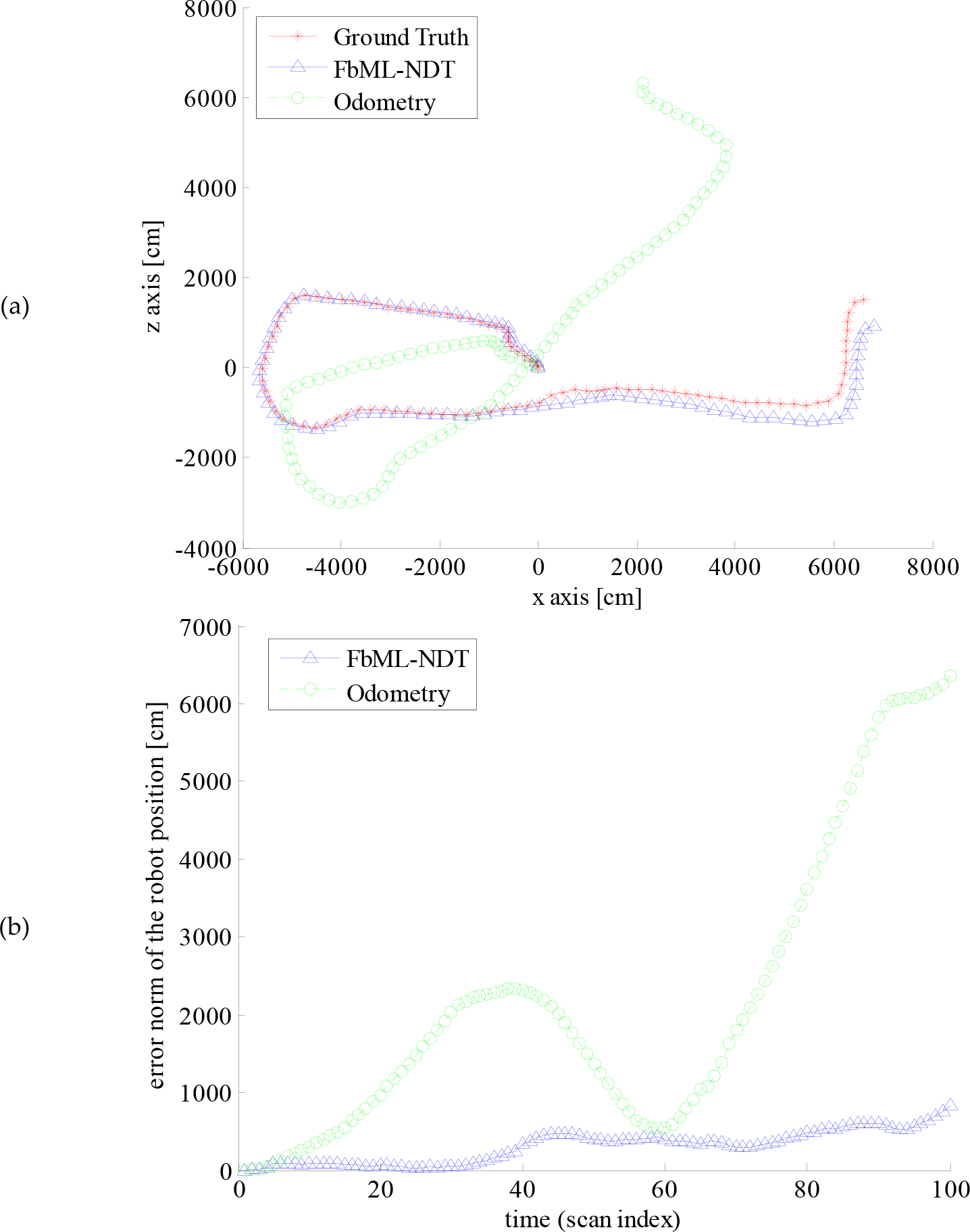
(a) Robot localization performance with odometry and FbML-NDT; (b) The norm of the robot position (x,y,z) error with respect to the ground truth position

Figure 12.

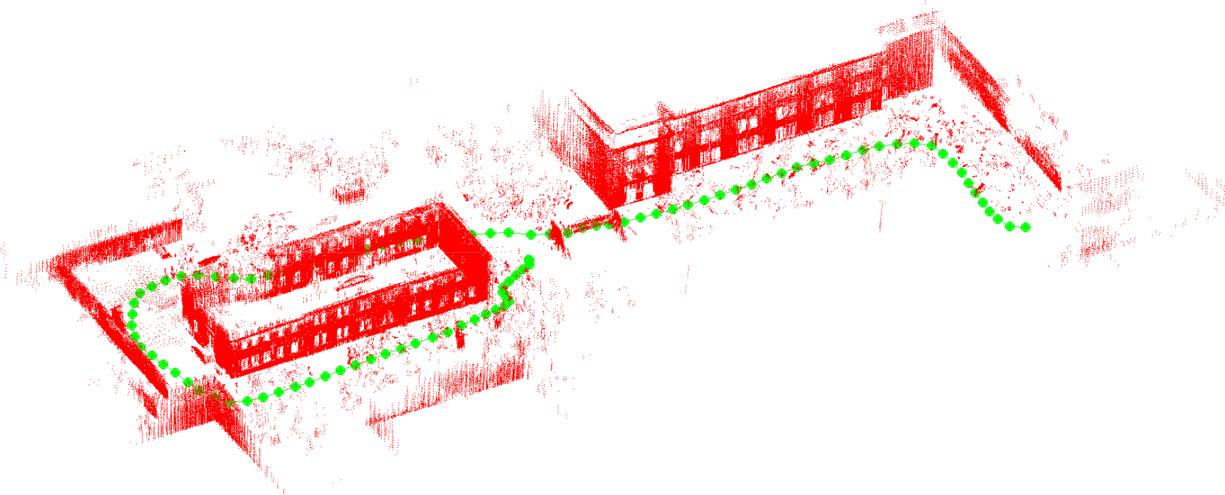
(a) Visual map. The plane feature points and robot positions (dots)

5. Conclusion and Future Works

In this study, a fast and robust scan-matching method based on feature extraction is proposed and the effect of sampling strategies on scan-matching is investigated. The scan-matching part is based on ML-NDT, and the feature extraction part is based on a plane detection method. These two methods are combined in such a way that the extracted plane inlier points are used in the registration process of the scan-matching algorithm. In this way, robust and fast scan-matching and feature extraction algorithms are obtained. From the scan-matching point of view, this method is robust because the matching is based on certain geometric structures, like planar surfaces, and faster with respect to the conventional methods because the number of matching points is reduced effectively and efficiently, which is very important due to the iterative structure of the scan-matching method.

For future study, we plan to focus on environments where large-planar features do not exist or else where there are relatively few plane structures. In this case, the problem is more challenging and the feature extraction method based on plane extraction and proposed in this study does not work. Therefore, we need to look for another modelling strategy. Another feature work will be on the usage of planar features in the future and based on SLAM and their combination with the proposed method. Moreover, an interesting issue, namely to solve the loop detection problem based on the extracted features, is being considered as future work.

Footnotes

6. Acknowledgments

This work was supported in part by the TUBITAK under grant number 110E194.

References

Ulas

Temeltas

, “A 3D Scan Matching Method Based On Multi-Layered Normal Distribution Transform,” presented at the 18th IFAC World Congress, 2011.

Ulas

Temeltas

, “A fast and robust scan matching algorithm based on ML-NDT and feature extraction,” In Mechatronics and Automation (ICMA), 2011 International Conference on, 2011, pp. 1751–1756.

Besl

P. J.

McKay

H. D.

, “A method for registration of 3-D shapes,” Pattern Analysis and Machine Intelligence, IEEE Transactions on, vol. 14, pp. 239–256, 1992.

Biber

Strasser

, “The normal distributions transform: a new approach to laser scan matching,” In Intelligent Robots and Systems, 2003. (IROS 2003). Proceedings. 2003 IEEE/RSJ International Conference on, 2003, pp. 2743–2748 vol.3.

Ulas

Temeltas

, “3D simultaneous localization and mapping based on multi-layered normal distribution transform,” In 18th Saint Petersburg International Conference on Integrated Navigation Systems, St. Petersburg, Russia, 2011, pp. 281–283.

Ohno

Nomura

Tadokoro

, “Real-Time Robot Trajectory Estimation and 3D Map Construction using 3D Camera,” In Intelligent Robots and Systems, 2006 IEEE/RSJ International Conference on, 2006, pp. 5279–5285.

Borrmann

Elseberg

Lingemann

Nuchter

Hertzberg

, “Globally consistent 3D mapping with scan matching,” Robot. Auton. Syst., vol. 56, pp. 130–142, 2008.

Chen

Medioni

, “Object modeling by registration of multiple range images,” In Robotics and Automation, 1991. Proceedings., 1991 IEEE International Conference on, 1991, pp. 2724–2729 vol.3.

Segal

Haehnel

Thrun

, “Generalized-ICP,” ed. Seattle, USA, 2009.

10.

Greenspan

Yurick

, “Approximate k-d tree search for efficient ICP,” In 3-D Digital Imaging and Modeling, 2003. 3DIM 2003. Proceedings. Fourth International Conference on, 2003, pp. 442–448.

11.

Takeuchi

Tsubouchi

, “A 3-D Scan Matching using Improved 3-D Normal Distributions Transform for Mobile Robotic Mapping,” In Intelligent Robots and Systems, 2006 IEEE/RSJ International Conference on, 2006, pp. 3068–3073.

12.

Brenner

, “Marker-free registration of terrestrial laser (b) braking in front a pedestrian (c) avoiding obstacle and pedestrian,” In In Proceedings of the ISPRS Working Group V/4 Workshop 3D-ARCH 2005, ed, 2005.

13.

Magnusson

Lilienthal

Duckett

, “Scan registration for autonomous mining vehicles using 3D-NDT: Research Articles,” J. Field Robot., vol. 24, pp. 803–827, 2007.

14.

Magnusson

, “The Three-Dimensional Normal Distributions Transform - an Efficient Representation for Registration, Surface Analysis, and Loop Detection,” Örebro Univeristy 2009.

15.

Kaminade

Takubo

Mae

Arai

, “The generation of environmental map based on a NDT grid mapping -Proposal of convergence calculation corresponding to high resolution grid,” In Robotics and Automation, 2008. ICRA 2008. IEEE International Conference on, 2008, pp. 1874–1879.

16.

Takubo

Kaminade

Mae

Ohara

Arai

, “NDT scan matching method for high resolution grid map,” In Intelligent Robots and Systems, 2009. IROS 2009. IEEE/RSJ International Conference on, 2009, pp. 1517–1522.

17.

Jinliang

Jihua

Yan

, “Study on localization for rescue robots based on NDT scan matching,” In Information and Automation (ICIA), 2010 IEEE International Conference on, 2010, pp. 1908–1912.

18.

Rusinkiewicz

Levoy

, “Efficient variants of the ICP algorithm,” In 3-D Digital Imaging and Modeling, 2001. Proceedings. Third International Conference on, 2001, pp. 145–152.

19.

Yakιn

İ.

, “Line Segment Based Range Scan Matching without Pose Information for Indoor Environments,” Bilkent Univ., 2008.

20.

Aghamohammadi

A. A.

Taghirad

H. D.

Tamjidi

A. H.

Mihankhah

, “Feature-Based Laser Scan Matching For Accurate and High Speed Mobile Robot Localization,” presented at the EMCR, 2007.

21.

Ozgur

, “A novel mobile robot navigation method based on combined feature based scan matching and FastSLAM algorithm,” M.S, Electrical And Electronics Engineering Middle East Technical University 2010.

22.

Pathak

Vaskevicius

Poppinga

Pfingsthorn

Schwertfeger

Birk

, “Fast 3D mapping by matching planes extracted from range sensor point-clouds,” In Intelligent Robots and Systems, 2009. IROS 2009. IEEE/RSJ International Conference on, 2009, pp. 1150–1155.

23.

Pathak

Birk

Vaskevicius

Pfingsthorn

Schwertfeger

Poppinga

, “Online three-dimensional SLAM by registration of large planar surface segments and closed-form pose-graph relaxation,” J. Field Robot., vol. 27, pp. 52–84, 2010.

24.

Sehgal

Cernea

Makaveeva

, “Real-Time Scale Invariant 3D Range Point Cloud Registration,” presented at the ICIAR (1), 2010.

25.

Viejo

Garcia-Rodriguez

Cazorla

, “A study of a soft computing based method for 3D scenario reconstruction,” Applied Soft Computing, vol. 12, pp. 3158–3164, 2012.

26.

Magnusson

Nuchter

Lorken

Lilienthal

A. J.

Hertzberg

, “Evaluation of 3D registration reliability and speed - A comparison of ICP and NDT,” In IEEE International Conference on Robotics and Automation, 2009, pp. 3907–3912.

27.

Weingarten

Siegwart

, “EKF-based 3D SLAM for structured environment reconstruction,” In Intelligent Robots and Systems, 2005. (IROS 2005). 2005 IEEE/RSJ International Conference on, 2005, pp. 3834–3839.

28.

Wang

C.-C.

, ed. Pittsburgh, PA: Robotics Institute, Carnegie Mellon University, 2004.

29.

Nüchter

. (2011). Robotic 3D Scan Repository. Available: http://kos.informatik.uni-osnabrueck.de/3Dscans/.

30.

Pandey

McBride

J. R.

Eustice

R. M.

, “Ford campus vision and lidar data set,” International Journal of Robotics Research, 2011.

31.

Fischler

M. A.

Bolles

R. C.

, “Random Sample Consensus: A Paradigm for Model Fitting with Applications to Image Analysis and Automated Cartography,” Communications of the ACM, vol. 24, pp. 381–395, 1981.

A Fast and Robust Feature-Based Scan-Matching Method in 3D SLAM and the Effect of Sampling Strategies

Abstract

Keywords

1. Introduction

2. Related Works

2.1 Scan-matching Methods for SLAM

2.2 Sampling Strategies for Scan-matching

2.3 Feature-based Scan-matching in SLAM

3. A Fast and Robust Feature-Based Scan-Matching Method

3.1 Multi-layered Normal Distribution Transform (ML-NDT)

3.2 Grid-based Sampling for ML-NDT

3.3 Feature Extraction

3.4 Feature-based Multi-layered Normal Distribution Transform (FbML-NDT)

4. Performance Analysis and Experimental Results

4.1 Performance of the FbML-NDT

4.2 Comparisons of Sampling Strategies with Feature Extraction

5. Conclusion and Future Works

Footnotes

6. Acknowledgments

References