Sage Journals: Discover world-class research

Abstract

This paper addresses a local environment recognition system for obstacle avoidance. In vision systems, obstacles that are located beyond the Field of View (FOV) cannot be detected precisely. To deal with the FOV problem, we propose a 3D Panoramic Environment Map (PEM) using a Modified SURF algorithm (MSURF). Moreover, in order to decide the avoidance direction and motion automatically, we also propose a Complexity Measure (CM) and Fuzzy-Logic-based Avoidance Motion Selector (FL-AMS). The CM is utilized to decide an avoidance direction for obstacles. The avoidance motion is determined using FL-AMS, which considers environmental conditions such as the size of obstacles and available space. The proposed system is applied to a humanoid robot built by the authors. The results of the experiment show that the proposed method can be effectively applied to a practical environment.

Keywords

Obstacle Avoidance 3D Panoramic Environment Map Avoidance Motion Selection Complexity Measure Humanoid Robot

1. Introduction

The study of humanoid robotics has recently evolved into an active area of research and development. Studies have been published in many related areas of research, such as autonomous walking, obstacle avoidance, stepping over obstacles, and walking up and down slopes and stairs. Yagi and Lumelsky [1] presented a robot that adjusts the length of its steps until it reaches an obstacle, depending on the distance to the closest obstacle in the direction of motion. If the size of the obstacle is small, the robot steps over the obstacle; if it is too tall to step over, the robot starts sidestepping until it clears the obstacle. Obviously, the decision to sidestep left or right is a pre-programmed one. Kuffner et al. [2] presented a footstep planning algorithm based on game theory that takes into account the global positioning of obstacles in the environment. Chestnutt et al. [3] and Michel et al. [4] presented vision-guided foot planning to avoid obstacles using Asimo Honda. These systems get environment information from a top-down view installed above the humanoid robot. Stasse et al. [5] and Kanehiro et al. [6] presented a stereo-vision-based locomotion planning algorithm that can modify the robot's waist height and upper body posture according to the size of the available space. Ayaz et al. [7] suggested a footstep approach suited to cluttered environments using a footstep planning algorithm that depends on the obstacle conditions. Gutmann et al. [8] suggested a modular architecture for humanoid robot navigation consisting of perception, control, and planning layers. The existing methods mentioned above use a global path planner that knows all the information on the walking environment. Global path planners, which provide information regarding the walking path and obstacles, have been used to guide humanoid robots to pre-defined goal positions [3, 8]. However, this assumption that the path planner knows all everything about the walking environment in advance is not appropriate if a humanoid robot walks through an unknown environment. Recently, local environment recognition systems have been studied. Wong et al. have proposed path planning systems using IR-sensor-based fuzzy controllers [19] and vision-based fuzzy controllers [20]. However, these systems do not supply decisions for avoidance direction and the first system does not provide accurate environment information due to the error of the IR sensor. Moreover, the vision-based fuzzy controller has problems with obstacles beyond the FOV and multi-obstacle avoidance.

Therefore, in this study, we focus on a local environment system for obstacle avoidance using a 3D-vision system. In particular, we address the Field of View (FOV) problem. Because the FOV problem occurs whenever humanoid robots meet obstacles that are too large, humanoid robots cannot precisely estimate the obstacle size and decide the appropriate motion. Therefore, we propose a Panoramic Environment Map (PEM) using a Modified Speeded-Up Robust Feature (MSURF). The conventional SURF [9] has weaknesses with respect to rotation and viewpoint change [10]; therefore, we modified the descriptor of the SURF algorithm by replacing the gradient-based method with a Modified Discrete Gaussian-Hermite Moment (MDGHM) method [11].

In [20], the vision-based fuzzy controller contained a fixed rotation angle according to the avoidance direction, which is inefficient when obstacles are of varying sizes. In this case, the humanoid robot finds it hard to escape various obstacles using only rotation motions with a fixed rotation angle. Therefore, the united avoidance motions of the humanoid robot need to be divided into avoidance direction and avoidance motion in terms of efficiency and adaptability of obstacle avoidance in an unknown walking environment. To achieve this, we propose a Complexity Measure (CM) and Fuzzy-Logic-based Avoidance Motion Selector (FL-AMS). The CM calculates the complexity of avoidance direction so that a humanoid robot can decide the avoidance direction by itself. The CM values measure the threat to the walking humanoid robot. A high CM value means that the walking environment for the humanoid robot is complex and difficult. As a result, the robot avoids the obstacle by walking in the direction with a lower CM value in terms of efficiency of motion. In addition, we also propose the FL-AMS method to avoid obstacles using environment information. The fuzzy-logic-based control method does not require a mathematical model and has the ability to approximate nonlinear systems. In addition, it can be easily implemented and extended without additional computational cost. In order to specify various motions in the robot, we define the avoidance motion as a combination of two motions based on four basic motions: sidestep walking (S), forward walking (F), rotation walking (R), and turning (T). The FL-AMS determines the optimal avoidance motion according to the environment information extracted from the PEM.

The remainder of this paper is organized as follows. In Section 2, we introduce the local environment recognition system. Section 3 gives the results of experiments to verify the performance of the proposed system. Section 4 concludes the paper by presenting contributions and plans for future work.

2. Local Environment Recognition System Using Modified SURF-Based 3D Panoramic Environment Map

To overcome the FOV problem, we generated a 3D Panoramic Environment Map (PEM) using a MDGHM-based SURF algorithm. From the PEM, we can obtain information about obstacles that exist beyond the limited FOV. Then, environment information, such as the location or sizes of obstacles, is extracted. Finally, avoidance motion planning, including avoidance direction and avoidance motion selection, is performed. Detailed methods are presented in the following subsections.

2.1 Architecture of Overall System

The overall local environment recognition system architecture is illustrated in Figure 1. The system largely consists of two parts: (1) PEM generation and extraction of environment information, and (2) determination of avoidance direction and avoidance motion. In the first part, we use an MSURF algorithm to generate the PEM. The MSURF algorithm has a modified version of the descriptor stage in the SURF algorithm. In [9], SURF was shown to be sensitive to rotation and viewpoint change caused by the gradient method. Therefore, we modified the conventional SURF using a moment-based method. The MSURF-based PEM generation gives environment information more precisely. To avoid obstacles in the determination of avoidance direction and avoidance motion, the robot calculates the CM values for the obstacles extracted from the PEM and determines the avoidance direction. In addition, we propose FL-AMS to select the optimal avoidance motion in various walking environments.

Figure 1.

Generation of Panoramic Environment Map

2.2 Modified DGHM-based SURF Algorithm

2.2.1 SURF Algorithm

With respect to processing speed, the SURF algorithm is a very efficient instrument to accomplish goals such as searching for point correspondence between distinct images. Its properties, e.g., repeatability, distinctiveness, and robustness, are stronger than those of previous, similar tools. The process of finding point correspondence between distinct images is composed of three main parts: first, interest point detection, the main component of the overall process; second, feature vector construction from existing interest points employing information about the local neighbourhood; and third, the matching of interest point pairs by relevant descriptors from each distinct image [9]. SURF strictly takes a role in only two parts: the detector and descriptor parts.

2.2.1.1 Detection

At the detection step, the major characteristic of SURF is a higher speed than previous algorithms. In order to obtain this, the key concept is an integral image adapted to the SURF algorithm. The integral image I_Σ(X) is computed by the summation of all pixels building the input image I at position X = (x,y)^T as

I_{Σ} (X) = \sum_{i = 0}^{i \leq x} \sum_{j = 0}^{j \leq j} I (i, j)

(1)

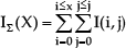
The processing time of the convolution calculation can be reduced sharply using box filtering. Figure 2 shows the integral image computation.

Figure 2.

Integral Image Computation

Another key component in the detection stage of SURF is the Hessian matrix that decides the interest points, i.e., features, required. It is made up of a box filter approximation of a convolution result between the Gaussian second order partial derivatives (x-axis and y-axis) and the image I.

Within a given image, the determinant of the Hessian matrix also plays a critical role when choosing interest points at each iteration. This is performed through non-maximum suppression (NMS) [9]. In addition, to extract interest points from an image, a Gaussian approximation filter is adapted to each level of filter size included in a scale space.

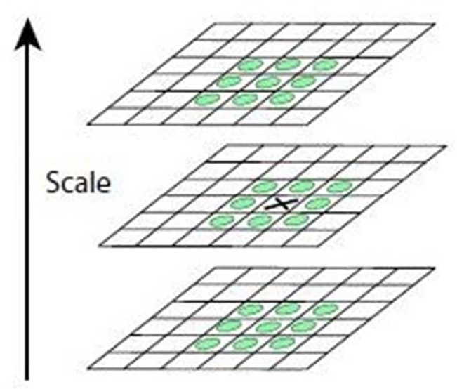
The scale space representation concept was also used in SIFT (Scale-Invariant Feature Transform); however, the scale space representation used in SURF is more computationally efficient and conserves more high-frequency components with no aliasing. Figure 3 shows the scale space representation of the SURF algorithm.

Figure 3.

Scale space representation of the SURF algorithm

As shown in Figure 3, by enlarging the size of the box filter instead of scaling down images, SURF operates with better speed than other feature detectors using the more prevalent concept of scale space. The final stage of detecting interest points is to compute NSM (non-maximum suppression) over the neighbourhood at three scales. To ensure that one interest point in the scale is the chosen feature, 3 × 3 × 3 neighbourhood pixels are processed, then one point selected by NMS becomes the keypoint, as shown in Figure 4.

Figure 4.

Feature extraction by NSM

2.2.1.2 Description

In order to assign invariability to the interest points, every interest point found by the detector is assigned a descriptor. When modifications happen to the scene, e.g., viewpoint angle change, scale change, blur increase, image rotation, image blur, compression, or illumination change, the descriptor of an interest point can be employed to identify correspondences between the original and transformed image. In SURF, this description is composed of two parts: orientation assignment and a Haar wavelet responses-based descriptor.

In orientation assignment, image orientation is specifically used to make an interest point invariable with respect to image rotation. Orientation is computed by detecting the dominant vector of the summation of the Gaussian-weighted Haar wavelet responses under a sliding window circle region spit into regions in increments of π/3 [9].

To calculate the descriptor of the interest point, the selected orientation and the square region centred around the interest point are needed. In the square region about the interest point, a 4 × 4 split square sub-region is assigned. This acts as the base stage for computing the horizontal Haar wavelet response, dx, and the vertical Haar wavelet response, dy. Then the dx and dy from each of the sub-regions are used to form the vector v=(Σdx, Σdy, Σ|dx|, Σ|dy|), called a descriptor. Some restrictions can be applied to the vector v to make extended versions of SURF, i.e., SURF-36 and SURF-128.

2.2.2 Modified DGHM (MDGHM)

The DGHM, including the Hermite polynomial and the Gaussian-Hermite Moment (GHM), was introduced in [12]. The pth degree Hermite polynomial, one of the orthogonal polynomials, is given as follows:

H_{p} (x) = {(- 1)}^{p} \exp (x^{2}) \frac{d^{p}}{d t^{p}} \exp (- x^{2})

(2)

Hermite polynomials satisfy the following orthogonality condition with respect to the weight function exp(–x²) as

\int_{- \infty}^{\infty} \exp (- x^{2}) H_{p} (x) H_{q} (x) d x = 2^{p} p! \sqrt{π} δ_{p q}

(3)

where δ_pq is the Kronecker delta.

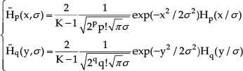
In order to obtain the orthonormal version, the normalized Hermite polynomial H_p(x) is calculated as

{\bar{H}}_{p} (x) = \frac{1}{\sqrt{2^{p} p! \sqrt{π} σ}} \exp (- \frac{x^{2}}{2}) H_{p} (x)

(4)

Gaussian-Hermite functions H_p(x/σ) can be calculated by replacing x with x / σ in (4).

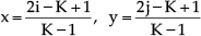
{\bar{H}}_{p} (x / σ) = \frac{1}{\sqrt{2^{p} p! \sqrt{π} σ}} \exp (- \frac{x^{2}}{2 σ^{2}}) H_{p} (x / σ)

(5)

In order to compute the moments for a digital image I(i,j) whose size is K×K [0≤i, j≤K − 1], the coordinate transformation over the square [–1≤x, y≤1] is performed using

x = \frac{2 i - K + 1}{K - 1}, y = \frac{2 j - K + 1}{K - 1}

(6)

The Discrete Gaussian-Hermite functions can be calculated using equidistance sampling as a substitute for the following equation.

{\begin{cases} {\overline{H}}_{p} (x, σ) = \frac{2}{K - 1} \frac{1}{\sqrt{2^{p} p! \sqrt{π} σ}} \exp (- x^{2} / 2 σ^{2}) H_{p} (x / σ) \\ {\overline{H}}_{q} (y, σ) = \frac{2}{K - 1} \frac{1}{\sqrt{2^{q} q! \sqrt{π} σ}} \exp (- y^{2} / 2 σ^{2}) H_{q} (y / σ) \end{cases}

(7)

From (5) and (7), the DGHM η_p,q, which is a discrete version of the GHM, can be derived as

η_{p, q} = \frac{4}{{(K - 1)}^{2}} \sum_{i = 0}^{K - 1} \sum_{j = 0}^{K - 1} I (i, j) {\overline{H}}_{p} (x, σ) {\overline{H}}_{q} (y, σ)

(8)

The DGHM is a global feature representation method for a square image in the discrete domain. Therefore, we need to modify the conventional DGHM to represent the local feature of a non-square image. The Modified DGHM (MDGHM), proposed by Kang in [11], is the DGHM of a mask with sampling intervals. Let I(i,j) be a digital 2D image and let t(u,v) be a mask whose size is M×N [0 ≤ u ≤ M − 1, 0 ≤ v ≤ N − 1]. The maximum number of samples, k_M, k_N, are calculated as follows:

k_{M} = M / m_{M}, k_{N} = N / m_{N}, for t (u, v)

(9)

where m_M and m_N are sampling intervals on the u – axis and v – axis respectively. The pixel values of the mask t(u, v)_(i.j) located at an arbitrary point on the input image I(i, j) are obtained as

t {(u, v)}_{(i, j)} = I (u + i - \frac{M}{2} + 1, v + j - \frac{N}{2} + 1)

(10)

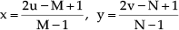
For the mask t(u, v)_(i,j), the coordinates are transformed such that −1 ≤ x, y ≤ 1, as follows:

x = \frac{2 u - M + 1}{M - 1}, y = \frac{2 v - N + 1}{N - 1}

(11)

and the Discrete Gaussian-Hermite functions of the mask t(u, v)_(i,j) can be written as follows:

{\begin{cases} {\overset{\land}{H}}_{p} (x, σ) = \frac{2}{M - 1} {\overline{H}}_{p} (x / σ) \\ = \frac{2}{M - 1} \frac{1}{\sqrt{2^{p} p! \sqrt{π} σ}} \exp (- x^{2} / 2 σ^{2}) H_{p} (x / σ) \\ {\overset{\land}{H}}_{q} (y, σ) = \frac{2}{N - 1} {\overline{H}}_{q} (y / σ) \\ = \frac{2}{N - 1} \frac{1}{\sqrt{2^{q} q! \sqrt{π} σ}} \exp (- y^{2} / 2 σ^{2}) H_{q} (y / σ) \end{cases}

(12)

From (10) and (12), the MDGHM with sampling intervals at arbitrary point on the input image I(i,j) can be written as follows:

\begin{array}{l} {\overset{\land}{η}}_{p, q} (i, j, m_{M}, m_{N}) = \frac{4}{(M - 1) (N - 1)} \sum_{u = 0}^{k_{M} - 1} \sum_{v = 0}^{k_{N} - 1} I (i + (m_{M} u - \frac{M}{2} + 1), \\ j + (m_{N} v - \frac{N}{2} + 1)) {\overset{\land}{H}}_{p} (x, σ) {\overset{\land}{H}}_{q} (y, σ) . \end{array}

(13)

2.2.3 Modified SURF (MSURF) Algorithm

In [10], SURF was shown to be sensitive to conditions such as rotation and viewpoint changes, stemming from the gradient method used in the description part of SURF. To solve this problem and improve the matching accuracy of the SURF algorithm, we propose a Modified SURF (MSURF) algorithm. Figure 5 presents an overview of the proposed MSURF algorithm.

Figure 5.

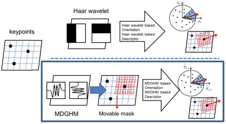
Overview of MSURF algorithm

As shown in Figure 5, we use MDGHM for orientation assignment and description in conventional SURF by calculating an MDGHM-based orientation and descriptor.

For orientation assignment, we replace the gradient-based, dx, dy filters based on the Haar wavelet response with MDGHM to represent the feature information more precisely. Figure 6 shows an example of the MDGHM-based box filter whose size is 2s × 2s.

Figure 6.

Examples of MDGHM-based box filter

Let (i_a, j_a) be the locations of a keypoint in a digital image I_D, where a is the index of the keypoints. From (13), the MDGHM-based box-filter response at (i_a, j_a) can therefore be calculated as follows:

\begin{array}{l} {\overset{\land}{η}}_{p, q} (i_{a}, j_{a}, m_{M}, m_{N}) = \frac{4}{(M - 1) (N - 1)} \sum_{u = 0}^{k_{M} - 1} \sum_{v = 0}^{k_{N} - 1} I_{D} (i_{a} + (m_{M} u - \frac{M}{2} + 1), \\ j_{a} + (m_{N} v - \frac{N}{2} + 1)) {\overset{\land}{H}}_{p} (x, σ) {\overset{\land}{H}}_{q} (y, σ) . \end{array}

(14)

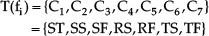
To extract the dominant direction, we calculate the magnitude m(i_a, j_a) and angle μ(i_a, j_a) as follows:

m (i_{a}, j_{a}) = \sqrt{{({\overset{\land}{η}}_{p, 0} (i_{a}, j_{a}))}^{2} + {({\overset{\land}{η}}_{0, q} (i_{a}, j_{a}))}^{2}}

(15)

\overset{\land}{μ} (i_{a}, j_{a}) = \arctan (\frac{({\overset{\land}{η}}_{0, q} (i_{a}, j_{a}))}{({\overset{\land}{η}}_{p, 0} (i_{a}, j_{a}))})

(16)

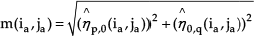
The size of the MDGHM-based box filter is defined as follows:

{\begin{cases} M = 2 \times r o u n d (p σ) + 1, for x-axis \\ N = 2 \times r o u n d (q σ) + 1, for y-axis \end{cases}

(17)

where p and q are the orders of the MDGHM and σ denotes the standard deviation. All keypoints with their own MDGHM-based magnitude and orientation are used when structuring the dominant orientation in the description step of conventional SURF. The rest of the description step of the SURF descriptor is similar to conventional SURF, except that we replace the gradient magnitude and orientation of the descriptor with the MDGHM-based magnitude and orientation.

2.3 PEM generation based on the MSURF-SURF algorithm and extraction of Environment Information

2.3.1 PEM generation based on the MSURF-SURF algorithm

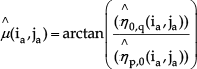
As mentioned above, because the FOV problem occurs whenever humanoid robots meet obstacles that are too large, humanoid robots cannot precisely estimate the obstacle's size and decide the appropriate reaction. To solve this problem, we propose the Panoramic Environment Map (PEM) using the MSURF algorithm. Table 1 shows the overall procedure of PEM generation. The procedure of PEM generation is similar to [13] until the fifth step in Table 1.

Table 1.

Algorithm: Panoramic Environment Map

Input: n ordered images

Output: 3D PEM image

Sequence:

– Extract MSURF feature all n depth images.

– Select m candidate matching pairs with the most features.

– Find geometrically consistent feature matches using RANSAC.

– Perform bundle adjustment.

– Render 3D panoramic image using multi-band blending.

– Find principal angular positions using FNCC.

– Find the other angular positions using linear interpolation.

The first step is to extract and match MSURF features between two images. Since MSURF features are more invariant to changes in scale, rotation, viewpoint, and illumination than those of traditional SURF, our method can handle images with varying orientation and zoom. To obtain a good solution for the image geometry at the second stage, it is only necessary to select a small number of matching pairs to stitch together a panoramic image using the invariant features of overlapping images. In the third stage, we only consider the n images that have the greatest number of feature matches to the current image for potential image matches (we use n = 9). In this stage, we use RANSAC to select a set of inliers that are compatible with a homography between the images. In the fourth stage, given a set of geometrically consistent matches between the images, we use bundle adjustment [13] to provide solutions for all of the camera parameters jointly. This is an essential step, since concatenation of pairwise homographies causes accumulated errors and disregards multiple constraints between images, e.g., that the ends of a panorama should join up. Images are added to the bundle adjuster one by one, with the best-matching image being added at each step. Then the parameters are updated using a least squares framework [13].

Ideally, each sample (pixel) along a ray would have the same intensity in every image that it intersects, but in reality this is not the case. Even after gain compensation, some image edges are still visible due to a number of un-modelled effects, such as vignetting, where intensity decreases towards the edge of the image, parallax effects due to unwanted motion of the optical centre, misregistration errors due to mismodelling of the camera, radial distortion, and so on. Because of this, a good blending strategy is important. In the final stage, we use the multi-band blending algorithm to solve the problem, which blends low frequencies over a large spatial range and high frequencies over a short range [13].

Figure 7 shows an example of the 3D panoramic images using nine 3D depth images. Figure 7(a) shows the input images gathered from the 3D TOF camera installed on the humanoid robot and Figure 7(b) image shows the resulting generated 3D panoramic image.

Figure 7.

The 3D panoramic image generation: (a) nine input images obtained from 3D TOF camera installed on the Humanoid Robot, and (b) generated 3D panoramic image

From the 3D panoramic image, we can extract the obstacles and their information. Let θ and φ be angles on the xz and yz planes, respectively. The key angular position for the nine 3D TOF images in the 3D panoramic image can be estimated using Fast Normalized Cross Correlation (FNCC) [14] as follows:

γ (u, v) = \frac{\sum_{x, y} [f (x, y) - \bar{f_{u, v}}] [t (x - u, y - v) - \bar{t}]}{{{\sum_{x, y} [f (x, y) - \bar{f_{u, v}}]}^{2} {[t (x - u, y - v) - \bar{t}]}^{2}}^{0.5}}

(18)

where f is the 3D panoramic image, t is an input depth image from the TOF sensor, t̄ is the mean of t, and f_u,v̄ is the mean of f(x,y) in the region under the depth image t. Each corresponded point is considered to have an angular position from −60 to 60 degrees with intervals of 30 degrees. The angular positions for θ and φ can be calculated from the PEM using linear interpolation as follows:

\begin{array}{l} θ = {\begin{cases} A_{i} + (A_{i + 1} - A_{i}) \times (x - x_{A_{i}}) / (x_{A_{i + 1}} - x_{A_{i}}), A_{i + 1} > A_{i} > 0 \\ A_{i} - (A_{i} - A_{i + 1}) \times (x_{A_{i}} - x) / (x_{A_{i}} - x_{A_{i + 1}}), 0 < A_{i + 1} < A_{i} \end{cases} \\ ϕ = {\begin{cases} B_{i} + (B_{i + 1} - B_{i}) \times (y - y_{B_{i}}) / (y_{B_{i + 1}} - y_{B_{i}}), B_{i + 1} > B_{i} > 0 \\ B_{i} - (B_{i} - B_{i + 1}) \times (y_{B_{i}} - y) / (y_{B_{i}} - y_{B_{i + 1}}), 0 < B_{i + 1} < B_{i} \end{cases} \end{array}

(19)

where A = {–60,–30,0,30,60} and B = {–17,0,17}. Figure 8 shows the results of the 3D PEM generation using (18) and (19).

Figure 8.

Environment information result from the PEM image

To calculate obstacle information such as size or location, we need to transform from spherical to Cartesian coordinates.

(\begin{array}{l} x \\ y \\ z \end{array}) = (\begin{matrix} r \sin θ \cos ϕ & 0 & 0 \\ 0 & r \sin θ \sin ϕ & 0 \\ 0 & 0 & r \cos θ \end{matrix})

(20)

2.3.2 Extraction of Environment Information

In order to extract the obstacles, we need to detect blobs in the 3D PEM. Blob detection is preceded by a Connected Component Labelling (CCL) algorithm [21]. Before blob detection, preprocessing such as level-set division is carried out because CCL operates on binary images. Let I(x_i,y_i,z_i), i = 1, …, N be an input 3D PEM with N pixels. The level-set is divided into m bins that affect the interval of each level-set. First, we define maximum available distance d_max = 2.5 m and m = 50. From the distance of each pixel z_i, level-set is defined as follows:

l e v e l s e t (I_{k}) = {\begin{cases} I_{k} (x_{}^{k}, y_{}^{k}, z_{}^{k}) \leftarrow I (x, y, z) k=j \\ 0 else \end{cases}

(21)

where k = 0, …, m − 1, j = floor(floor(z_i)/Δd), and Δd = d_max / m. From the level-set, obstacles are indexed by CCL as follows:

o_{l}^{k} (x_{l}^{k}, y_{l}^{k}, z_{l}^{k}) = C C L (I_{k} (x_{}^{k}, y_{}^{k}, z_{}^{k}))

(22)

In (22), o₁^k is the l th obstacle in the kth level-set extracted by CCL. These indexed obstacles are used as the input data for decisions regarding avoidance direction and obstacle analysis. From (22), we can calculate the width, distance, and location of the obstacles. Figure 9 shows the parameters used to calculate the location and width for each extracted obstacle, including the angle, size, and distance between obstacles and the distance between the robot and the obstacle.

Figure 9.

Environment information: location and width calculation

Firstly, the perpendicular distance d_x₁^k is calculated as follows:

d_{x_{l}^{k}} = d_{z_{l}^{k}} \sin θ_{F O V} \times (# p_{c o_{l}^{k}} / # p_{F O V})

(23)

From (23), the maximum width of FOV w_FOV at the perpendicular distance d_x₁^k can be calculated as follows:

w_{F O V} = 2 \times \tan (θ_{F O V} / 2) \times d_{z_{l}^{k}}

(24)

Using (24), the width of the obstacles w₁^k can be calculated by using the ratio between the number of pixels of the FOV and the number of pixels of the obstacle o₁^k as follows:

w_{k}^{l} = w_{F O V} \times (# p_{o_{l}^{k}} / # p_{F O V})

(24)

We can also calculate the angle θ_k¹ between the centre of the robot and the centre of an obstacle.

θ_{l}^{k} = \arctan (d_{x_{l}^{k}} / d_{z_{l}^{k}})

(25)

2.4 Determination of Avoidance Direction and Avoidance Motion

2.4.1 Determination of Avoidance Direction Using the Complexity Measure (CM)

The environment information from obstacle extraction and size estimation is used as the input data to decide the best direction for avoiding obstacles. To decide the avoidance direction, we propose the complexity measure (CM) as follows:

C M = {\begin{cases} \sum_{k = 1}^{m} \sum_{l = 1}^{n} 2^{k} + 2^{(π / 2 - θ_{l}^{k})} + w_{l}^{k}, θ_{l}^{k} > 0 \\ - \sum_{k = 1}^{m} \sum_{l = 1}^{n} 2^{k} + 2^{(π / 2 + θ_{l}^{k})} + w_{l}^{k}, θ_{l}^{k} < 0 \\ \sum_{k = 1}^{m} \sum_{l = 1}^{n} 2^{k} + w_{l}^{k}, θ_{l}^{k} = 0 \end{cases}

(26)

As shown in (26), the CM is determined by three factors: the distance between the robot and the obstacle, the width and the height of the obstacle, and the angle of the obstacle from the robot's current direction. The CM has a large value in cases where the robot is close to the obstacle, where the angle from the centre of the PEM to the obstacle is small, and where the obstacle is large in size. A large CM value indicates that the environment is too complex for the robot to avoid the obstacle. Therefore, we get the final avoidance decision from the determination value D as follows:

D = s i g n (\sum_{a l l o b s t a c l e} C M) = {\begin{cases} D < 0, turn right \\ D > 0, turn left \end{cases}

(27)

In (27), the CMs for obstacles located on the left side of the robot have negative values, and the CMs for obstacles located on the right side of the robot have positive values. Therefore, the avoidance direction can be determined by the summation of all CMs over all obstacles. If D is positive, the robot turns to the left, and if D is negative, the robot turns to the right.

2.4.2 Decision of Avoidance Motion Using a Fuzzy-Logic-Based Avoidance Motion Selector (FL-AMS)

After choosing the direction to take to avoid the obstacle, a motion type must be selected based on the environment conditions. To achieve this purpose, we need an intelligent control approach. Fuzzy logic is one such approach that does not require mathematical modelling and has the ability to approximate nonlinear systems. In addition, it can be easily implemented and extended without additional computational cost. Therefore, we propose a fuzzy-logic-based avoidance motion selector (FL-AMS).

In order to perform fuzzification [15], the difference w_i between the obstacle width and robot width and the space difference S_i between the avoidance space width and the robot width are set up as the input variables. Figure 10 shows the input and output membership functions. As shown in Figure 10, triangular-type membership functions and fuzzy-singleton-type membership functions are used for the input and output variables, respectively. The term sets of the input and output variables are selected as follows:

Figure 10.

Membership functions of fuzzy system: (a) Input variable w_i, (b) input variable s_i, and (c) output variable f_i

T (w_{i}) = {A_{1}, A_{2}, A_{3}, A_{4}, A_{5}} = {N L, N S, Z, P S, P L}

(27)

T (s_{i}) = {B_{1}, B_{2}, B_{3}, B_{4}, B_{5}} = {N L, N S, Z, P S, P L}

(28)

\begin{array}{l} T (f_{i}) = {C_{1}, C_{2}, C_{3}, C_{4}, C_{5}, C_{6}, C_{7}} \\ = {S T, S S, S F, R S, R F, T S, T F} \end{array}

(29)

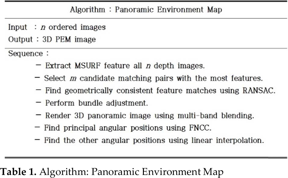
where fuzzy sets A₁, A₂, A₃, A₄, and A₅ are respectively denoted as Negative Large (NL), Negative Small (NS), Zero (Z), Positive Small (PS), and Positive Large (PL) for the input variable w_i. Fuzzy sets B₁, B₂, B₃, B₄, and B₅ are also respectively denoted as Negative Large (NL), Negative Small (NS), Zero (Z), Positive Small (PS), and Positive Large (PL) for the input variable d_i. Fuzzy sets C₁, C₂, C₃, C₄, C₅, C₆, and C₇ are respectively denoted as Stop (ST), Slip step + Slip step (SS), Slip step + Forward step (SF), Rotation step + Slip step (RS), Rotation step + Forward step (RF), Turning step + Slip step (TS), and Turning step + Forward step (TF). All of these are combinations of any two motions: Slip step (S), Forward step (F), Rotation step (R), Turning step (T), but excluding the Stop motion (ST) for the output variable f_i.

\begin{array}{l} Rule R (j_{1}, j_{2}) : \\ IF w_{i} is A_{j_{1}} and d_{i} is B_{j 2}, then f_{i} is C_{f (j_{1}, j_{2})} \\ j_{1} \in {1, 2, 3, 4, 5}, j_{2} \in {1, 2, 3, 4, 5}, f (j_{1}, j_{2}) \in {1, 2, 3, 4, 5, 6, 7} \end{array}

(30)

To determine the final output of the FL-AMS, we use the weighted average method described by:

f_{i} = f (w_{i}, s_{i}) = \frac{\sum_{j_{1} = 1}^{j_{1} = 5} \sum_{j_{2} = 1}^{j_{2} = 5} u (j_{1}, j_{2}) • v (C_{f (j_{1}, j_{2})})}{\sum_{j_{1} = 1}^{j_{1} = 5} \sum_{j_{2} = 1}^{j_{2} = 5} u (j_{1}, j_{2})}

(31)

where v(C_f(j₁,j₂)) is the crisp value of the fuzzy set, C_f(j₁,j₂). The function u(j₁, j₂) is the fire strength of the rule R(j₁, j₂) and can be described by:

u (j_{1}, j_{2}) = \min (μ_{A_{j_{1}}} (w_{i}), μ_{B_{j 2}} (s_{i}))

(32)

Based on the width difference w_i between obstacle width and robot width and space difference s_i between avoidance space width and robot width, the seven evaluation values f_i, i ∈ {1,2,3,4,5,6,7} for the seven avoidance motions can be determined by the FL-AMS.

Walking motion types consist of seven motions, SS, SF, RS, RF, TS, and TF, which are combinations of two of the motions sidestep walking (S), forward walking (F), rotation walking (R), and turning (T), excluding the stop motion (ST). Table 2 shows the fuzzy rule table for the walking motions.

Table 2.

Fuzzy rule table for FL-AMS

f_i		s_i
f_i		NL	NS	z	PS	PL
w_i	NL	ST	SS	SF	SF	SF
	NS	ST	SS	SF	SF	SF
	Z	ST	RS	RF	RF	RF
	PS	ST	RS	RF	RF	RF
	PL	ST	TS	TF	TF	TF

3. Experimental Results for Intelligent Obstacle Avoidance

We carried out experiments to investigate the effectiveness of local environment recognition using the proposed MSURF algorithm. Our experiment largely consists of accuracy testing for environment information and the success rate of obstacle avoidance for the designed humanoid robot. A detailed description of these is presented below.

3.1 Humanoid Robot Design

For this experiment, we designed and built a humanoid robot. The overall construction of our humanoid robot is shown in Figure 11.

Figure 11.

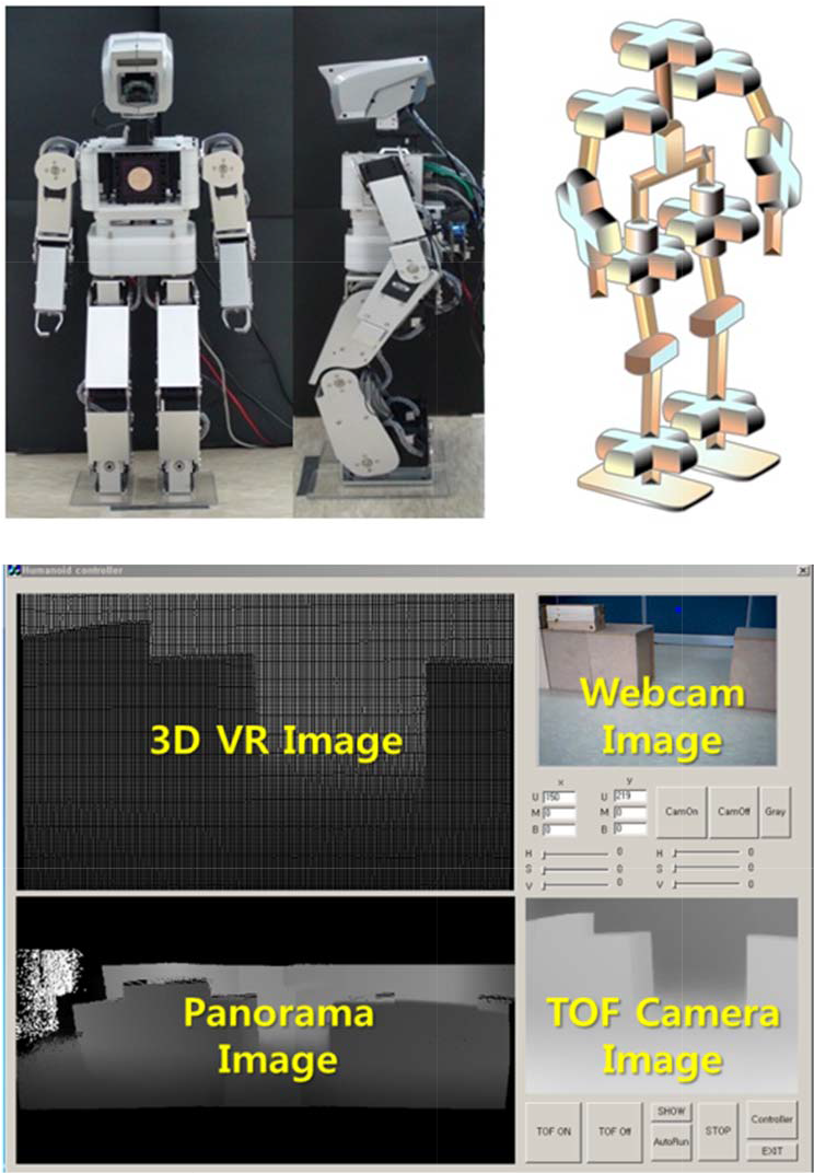
Humanoid Robot Design and GUI

The height of the humanoid robot is about 600 mm. Each joint is driven by the RC servomotor, which consists of a DC motor, gear, and simple controller. Our humanoid robot also has 23 degrees of freedom (DOF) and two different vision systems, a 3D TOF camera and a webcam. As shown in Figure 11, the GUI largely consists of four parts: the 3D VR image, the webcam image, the TOF camera image, and the 3D PEM. The designed humanoid robot system has two vision systems: a webcam and a 3D TOF camera, which are shown on the webcam image part and TOF camera image part of the GUI, respectively. The 3D PEM image part shows the PEM generated by using the MSURF algorithm. Finally, the 3D VR image part, implemented using the OpenGL library [18], shows the analysed environmental information. Table 3 shows the specifications of our humanoid robot system.

Table 3.

Specification of the designed humanoid robot

Type	Specification
Size	Height: 600 mm
CPU	AT91SAM7s256 (ARM7 core)
Actuator (RC Servo motors)	RC Servo motors (RX-28 ^* 3, RX-64 ^* 8, RX-106 ^* 12)
Degree of Freedom	23 DOF (Leg + Arm + Head + Waist)
Degree of Freedom	= 2^6 + 2^4 + 2 + 1
Power Source	Power supply (17 V)
Sensors	3D: TOF camera (SR-4000)
Sensors	2D: Webcam

3.2 Experimental Setup

We implemented our obstacle avoidance approach using the humanoid robot with a TOF camera. The vision system on the robot's head provides disparity images (176 × 144) at 30fps. For testing our perception method, we set up an obstacle environment containing obstacles and avoidance spaces of different sizes.

As shown in Figure 12, the experiment space was 2.5 m × 3 m and there were two types of artificial obstacles which had dimensions of 32 cm (W) × 32 cm (H) × 24 cm (D).

Figure 12.

Experiment environment

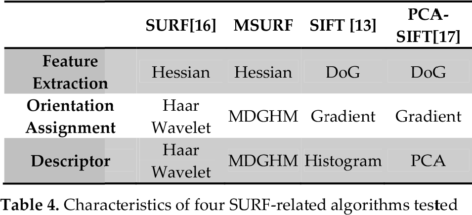
These were used in various combinations so that we could make obstacles of different widths and spacing. We evaluated four related algorithms: a SIFT-based method, a PCA-SIFT-based method, a conventional SURF-based method, and the proposed MSURF-based method, as tabulated in Table 4. We set the MSURF parameters to p = q = 3, σ = 0.3, m_M = m_N = 1 and used a window size of 5s×5s.

Table 4.

Characteristics of four SURF-related algorithms tested

	SURF[16]	MSURF	SIFT [13]	PCA-SIFT[17]
Feature Extraction	Hessian	Hessian	DoG	DoG
Orientation Assignment	Haar Wavelet	MDGHM	Gradient	Gradient
Descriptor	Haar Wavelet	MDGHM	Histogram	PCA

3.3 Experiment Results for Environment Information

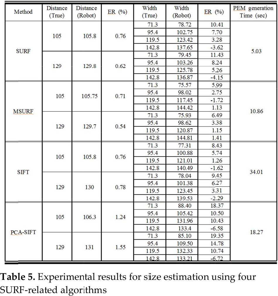
To estimate obstacle information, we proposed the PEM image using the MDGHM-SURF algorithm. In this section, we tested the accuracy of the obstacle size estimation of the proposed method and compared the results with those of the PEM image using the SIFT algorithm. In this experiment, we tested the performance of size estimation for four types of obstacles with widths of 71.3 cm, 95.4 cm, 119.5 cm, and 142.8 cm, respectively, 20 times for each width.

Table 5 shows the results for size estimation for various distances and sizes using the four SURF-related algorithms. In Table 5, the results for the estimated distance, the estimated width of obstacles, and PEM generation times were averaged over 20 trials. As shown in Table 5, although the generation time for the MSURF-based method is a little slower than the SURF-based method, the MSURF-based method shows better performance than the others with respect to the size estimation of the obstacles. Figure 13 shows some example PEM images using the MSURF algorithm.

Figure 13.

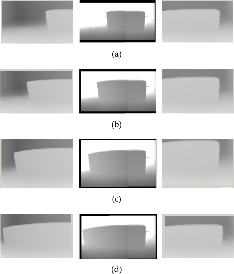
Example PEM images made using MSURF for an obstacle at 105 cm distance: widths of obstacle are (a) 71.3 cm, (b) 95.4 cm, (c) 119.5 cm, and (d) 142.8 cm

Table 5.

Experimental results for size estimation using four SURF-related algorithms

Method	Distance (True)	Distance (Robot)	ER (%)	Width (True)	Width (Robot)	ER (%)	PEM generation Time (sec)
SURF	105	105.8	0.76	71.3	78.72	10.41	5.03
				95.4	102.75	7.70
				119.5	123.42	3.28
				142.8	137.65	-3.62
	129	129.8	0.62	71.3	79.45	11.43
				95.4	103.26	824
				119.5	125.78	5.26
				142.8	136.87	-4.15
MSURF	105	105.75	0.71	71.3	75.57	5.99	10.86
				95.4	98.02	2.75
				119.5	117.45	-1.72
				142.8	144.42	1.13
	129	129.7	0.54	71.3	75.93	6.49
				95.4	98.62	3.38
				119.5	120.87	1.15
				142.8	144.81	1.41
SIFT	105	105.8	0.76	71.3	77.31	8.43	34.01
				95.4	100.88	5.74
				119.5	121.01	1.26
				142.8	140.49	-1.62
	129	130	0.78	71.3	78.04	9.45
				95.4	101.38	6.27
				119.5	123.45	3.31
				142.8	139.53	-2.29
PCA-SIFT	105	106.3	1.24	71.3	88.40	18.37	18.27
				95.4	105.42	10.50
				119.5	131.96	10.43
				142.8	133.4	-6.58
	129	131	1.55	71.3	85.10	19.35
				95.4	109.50	14.78
				119.5	132.33	10.74
				142.8	133.21	-6.72

3.4 Experiment Results for Decisions of Avoidance Direction and Avoidance Motion

We tested our proposed method under various environmental conditions. The humanoid robot was programmed to walk and stop when it met an obstacle within a fixed or defined distance. Then the humanoid robot determined the decision factors needed to avoid obstacles. We carried out the experiments regarding the decision and control performance under various obstacle conditions.

First, we verified the performance of the FL-AMS method proposed in this paper for walking obstacle avoidance using the humanoid robot. In Table 6, a confusion matrix shows that the proposed algorithm confidently predicts the correct motion decision. In Table 6, one thousand random values consisting of the obstacle size and the avoidance space were used as the input, and the outputs are tabulated for each situation.

Table 6.

Confusion matrix for motion decisions

				Predicted	Motion
Actual Motion		SS	SF	RS	RF	TS	TF	ST
	SS	980	0	11	0	0	0	9
	SF	2	987	0	11	0	0	0
	RS	6	0	984	0	0	0	10
	RF	0	6	3	991	0	0	0
	TS	0	0	2	0	988	0	10
	TF	0	0	0	3	3	994	0
	ST	2	0	1	0	2	0	995

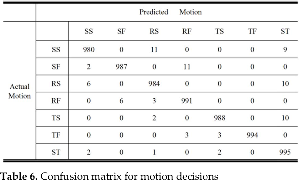
As shown in Table 6, the FL-AMS shows good decision accuracies, 98% (980/1000) for SS motion, 98.7% (987/1000) for SF motion, 98.4% (984/1000) for RS motion, 99.1% (991/1000) for RF motion, 98.8% (988/1000) for TS motion, 99.4% (994/1000) for TF motion, and 99.5% (995/1000) for ST motion.

Secondly, we tested the decision and control performance under various obstacle conditions: obstacle width and avoidance space.

The experimental results are shown in Table 7, Figure 14, and Figure 15. We tested the obstacle avoidance walk of the humanoid robot under each condition 50 times. If the humanoid robot arrived at the destination we defined for it, the walking test succeeded. On the other hand, if the humanoid robot collided with an obstacle or got lost during walking, it failed. As shown in Table 7, the proposed method has a high success rate even without an optimal control method for walking. To improve the success rate of a humanoid robot system, a vision-based adaptive walking control system is needed for future work.

Figure 14.

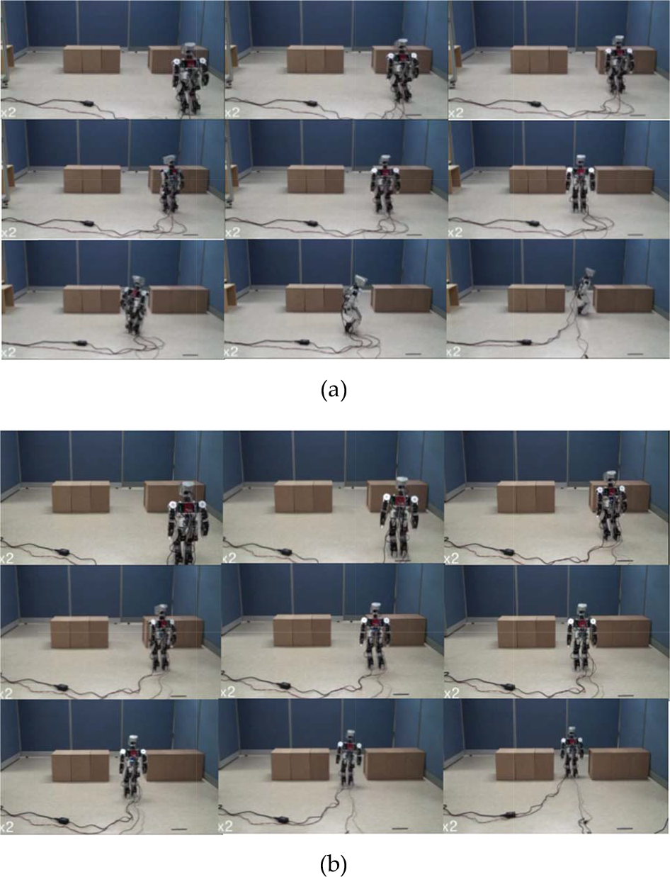
Experimental Results under various obstacle conditions: (a) SS motion type, (b) SF motion type

Figure 15.

Experimental Results under various obstacle conditions: (a) RS motion type, (b) RF motion type

Table 7.

Experimental results for obstacle avoidance

Motion	Trial	Method	Success	Rate (%)
SS	50	SURF	40	80
		MDGHM-SURF	42	84
		SIFT	40	80
		PCA-SIFT	37	74
SF	50	SURF	41	82
		MDGHM-SURF	46	92
		SIFT	43	86
		PCA-SIFT	39	78
RS	50	SURF	35	70
		MDGHM-SURF	41	82
		SIFT	36	72
		PCA-SIFT	33	66
RF	50	SURF	38	76
		MDGHM-SURF	44	88
		SIFT	40	80
		PCA-SIFT	35	70
TS	50	SURF	34	68
		MDGHM-SURF	39	78
		SIFT	35	70
		PCA-SIFT	32	64
TF	50	SURF	34	68
		MDGHM-SURF	38	76
		SIFT	34	68
		PCA-SIFT	31	62

Figure 14 illustrates a resulting image sequence when using SS and SF motion types, and Figure 15 presents an image sequence that resulted when using RS and RF motion types. In the cases shown in Figures 14 and 15, the results show good avoidance performance because the widths of the obstacles are reasonable for the humanoid robot.

4. Conclusion

In this paper, we introduced the local environment recognition system using an MSURF-based PEM for obstacle avoidance of a humanoid robot. The proposed method is based on a PEM image using an MSIFT algorithm, vision-based CM, and FL-AMS. The PEM image method can be a solution for overcoming the FOV problem, which may be a major cause of incorrect decisions in walking control and perception of environment.

The vision-based CM system decides the avoidance direction for a humanoid robot to avoid obstacles by considering environment information such as the distribution of obstacles, distance from the humanoid robot to the obstacles, and size of each obstacle.

Finally, the FL-AMS system automatically decides the best avoidance motion depending on the obstacle conditions using the environment information obtained by the PEM. These systems do not need a global path planner with all information regarding the obstacle location and path information in advance. From the experimental results, we believe that our proposed methods will be useful for humanoid robots in real environments.

References

Yagi

Lumelsky

(1999) Biped Robot Locomotion in Scenes with Unknown Obstacles. Proceedings of IEEE International Conference on Robotics and Automation (ICRA). pp. 375–380.

Kuffner

Nishiwaki

Kagami

Inaba

Inoue

(2001) Footstep Planning Among Obstacles for Biped Robots. Proceedings of IEEE/RSJ International Conference on Intelligent Robots and Systems (IROS). pp. 500–505.

Chestnutt

Lau

Cheung

Kuffner

Hodgins

Kanade

(2005) Footstep Planning for the Honda ASIMO Humanoid. Proceedings of the 2005 IEEE International Conference on Robotics and Automation. pp. 629–634.

Michel

Chestnutt

Kuffner

Kanade

(2005) Vision-guided Humanoid Footstep Planning for Dynamic Environments. Proceedings of the 5th IEEE-RAS International Conference on Humanoid Robots. pp. 13–18.

Stasse

Verrelst

Vanderborght

Yokoi

(August 2009) Strategies for Humanoid Robots to Dynamically Walk Over Large Obstacles. IEEE Transactions on Robotics. 25: 4: 960–967.

Kanehiro

Yoshimi

Kajita

Morisawa

Fujiwara

Harada

Kaneko

Hirukawa

Tomita

(April 2005) Whole Body Locomotion Planning of Humanoid Robots based on a 3-D Grid Map. Proceedings of the 2005 IEEE International Conference on Robotics and Automation. pp. 1072–1078.

Ayaz

Konno

Munawar

Tsujita

Uchiyama

(2009) Planning Footsteps in Obstacle Cluttered Environments. Proceedings of the IEEE/ASME International Conference on Advanced Intelligent Mechatronics. pp. 156–161.

Gutmann

Fukuchi

Fujita

(2008) 3-D Perception and Environment Map Generation for Humanoid Robot Navigation. International Journal of Robotics Research. 27: 10: 1117–1134.

Bay

Tuytelaars

Gool

(2008) Speeded Up Robust Features (SURF). Computer Vision and Image Understanding. 110: 346–359.

10.

Juan

Gwun

(2009) A Comparison of SIFT, PCA-SIFT, and SURF. International Journal of Image Processing. 3: 4: 143–152.

11.

Kang

Zhang

Kim

Park

(2012) Enhanced SIFT Descriptor Based on Modified Discrete Gaussian-Hermite Moment. ETRI Journal. 34: 4: 572–582.

12.

Yang

Dai

(2011) Image Analysis by Gaussian-Hermite Moments. Signal Processing. 91: 10: 2290–2303.

13.

Brown

Lowe

(2007) Automatic Panoramic Image Stitching using Invariant Features. International Journal of Computer Vision. 74: 1: 59–73.

14.

Zhang

Lafruit

Lauwereins

Gool

(2009) Robust Stereo Matching with Fast Normalized Cross-Correlation Over Shape-Adaptive Regions. Proceedings of the 16th IEEE International Conference on Image Processing. pp. 2357–2360.

15.

Mendel

(2001) Uncertain Rule-Based Fuzzy Logic Systems: Introduction and New Directions, Prentice-Hall.

16.

Juan

Gwun

(2010) SURF Applied in Panorama Image Stitching. Proceedings of Image Processing Theory, Tools, and Applications. pp. 495–499.

17.

Sukthankar

(2004) PCA-SIFT: A More Distinctive Representation for Local Image Descriptors. Proceedings of the International Conference on Computer Vision and Pattern Recognition. pp. II-506–513.

18.

http://www.opengl.org/.

19.

Wong

Cheng

Huang

Yang

(2008) Fuzzy Control of Humanoid Robot for Obstacle Avoidance. International Journal of Fuzzy Systems. 10: 1: 1–10.

20.

Wong

Hwang

Huang

Cheng

(2011) Design and Implementation of Vision-Based Fuzzy Obstacle Avoidance Method on Humanoid Robot. International Journal of Fuzzy Systems. 13: 1: 45–54.

21.

Shapiro

Stockman

(2002) Computer Vision. Prentice Hall.

Local Environment Recognition System Using Modified SURF-Based 3D Panoramic Environment Map for Obstacle Avoidance of a Humanoid Robot

Abstract

Keywords

1. Introduction

2. Local Environment Recognition System Using Modified SURF-Based 3D Panoramic Environment Map

2.1 Architecture of Overall System

2.2 Modified DGHM-based SURF Algorithm

2.2.1 SURF Algorithm

2.2.1.1 Detection

2.2.1.2 Description

2.2.2 Modified DGHM (MDGHM)

2.2.3 Modified SURF (MSURF) Algorithm

2.3 PEM generation based on the MSURF-SURF algorithm and extraction of Environment Information

2.3.1 PEM generation based on the MSURF-SURF algorithm

2.3.2 Extraction of Environment Information

2.4 Determination of Avoidance Direction and Avoidance Motion

2.4.1 Determination of Avoidance Direction Using the Complexity Measure (CM)

2.4.2 Decision of Avoidance Motion Using a Fuzzy-Logic-Based Avoidance Motion Selector (FL-AMS)

3. Experimental Results for Intelligent Obstacle Avoidance

3.1 Humanoid Robot Design

3.2 Experimental Setup

3.3 Experiment Results for Environment Information

3.4 Experiment Results for Decisions of Avoidance Direction and Avoidance Motion

4. Conclusion

References