
Abstract
Abstract In many manufacturing and automobile industries, flexible components need to be positioned with the help of coordinated operations of manipulators. This paper deals with the robust design of a control system for two planar rigid manipulators moving a flexible object in the prescribed trajectory while suppressing the vibration of the flexible object. Dynamic equations of the flexible object are derived using the Hamiltonian principle, which is expressed as a partial differential equation (PDE) with appropriate boundary conditions. Then, a combined dynamics is formulated by combining the manipulators and object dynamics without any approximation. The resulting dynamics are thus described by the PDEs, having rigid as well as flexible parameters coupled together. This paper attempts to develop a robust control scheme without approximating the PDE in order to avoid measurements of flexible coordinates and their time derivatives. For this purpose, the two subsystems, namely slow and fast subsystems, are identified by using the singular perturbation technique. Specific robust controllers for both the subsystems are developed. In general, usage of the singular perturbation technique necessitates exponential stability of both subsystems, which is evaluated by satisfying Tikhnov's theorem. Hence, the exponential stability analysis is performed for both subsystems. Focusing on two three-link manipulators holding a flexible beam, simulations are performed and simulation results demonstrate the versatility of the proposed robust composite control scheme.
Keywords
1. Introduction
The past four decades saw the tremendous growth of the use of robots in automobile, electronic, construction, manufacturing and medical applications. Robotic manipulator systems relieved humans of boring repetitive tasks, tasks in dangerous environments such as space and underwater, and tasks in high radiation environments. In some situations a single robot may not be able to grasp and move slender flexible objects along a prescribed trajectory in a safe and efficient way. Owing to the single arm structure, present day robots are called handicapped operators for performing complex tasks. Most tasks in assembly/disassembly, handling large or heavy objects are done efficiently with the help of two robot arms. Collaborative manipulators have the following advantages compared to single arm manipulators: increased load carrying capacity, reduced need for extra auxiliary equipment, efficient use of available workspace and safer handling of delicate and flexible objects. Considering these facts, two manipulator systems are employed in a wide range of tasks and the first master/slave teleoperated manipulator was used in the nuclear industry in the 1940s at Oak Ridge and Argonne National Laboratories [1].
In modern automobile body assembly there are more than 200 sheet metal parts which must be assembled in a precise way. Handling them needs special equipment and skilled operations. Two collaboratively operated robots can grasp flexible pieces of sheet metal and manipulate them together for assembly. Furthermore, in industry many deformable objects, such as rubber tubes, sheet metal, cords and leather products, are handled by special equipment or human operators. Satellite solar arrays and the aerospace industry have composite materials with allowable flexibility that must be handled with the help of at least two robotic manipulators. In order to effectively manipulate complex flexible objects and bend them in a desired manner, for example, in the insertion of a flexible beam into a hole and the assembling of sheet metal in the required place, at least two robot arms are needed. Robot assisted surgery is another area where collaborative robots in a vibration free environment will be useful.
Early studies on the collaboration of two arms handling objects mainly focused on rigid bodies. Some of them can be found in [2] and [3] and their references. There are some studies on the handling of flexible objects in the literature. Two manipulators handling flexible objects is a complex problem compared with manipulating rigid objects. In particular, the dynamics and control of flexible objects are more tedious than that for rigid objects. In 1991, Zheng et al. [4] studied inserting flexible cables or pegs into a small hole by using a single arm robot. Dellinger and Anderson [5] developed a mathematical model for the case of two manipulators handling a non-rigid object and they also analysed the interactive forces between the manipulators and the object. Zheng and Chen [6] extended the work of [4] on single arm manipulation to two arm manipulation for the alignment of flexible sheets in printed circuit boards. Yukawa et al. [7] proposed a position control algorithm to achieve total system stability and they also suppressed the vibration at the intermediate points of the flexible beam. Kosuge et al. [8] employed finite element model of the sheet metal and also implemented their control algorithm experimentally to reduce the vibration of the object. Sun and Liu [9] and [10] developed a new approach of modelling the beam using assumed modes and proposed a hybrid impedance controller which is used to stabilize the system while suppressing the vibrations and controlling internal forces. Azadi et al. [11] considered robust control of two 5 DOF robot manipualtors. Caccavale et al. [14] studied the impedance behaviour of dual arm cooperative manipulators. Gueaieb [12] et al. developed hybrid control and recently Moosavian et al. [16] and Yagiz [17] et al. considered nonlinear control for the cooperative manipualtor scenario. Al-Yahmali and Hsia [13] derived the sliding mode control algorithm to provide robustness against the model imperfections and uncertainty. The stability of the system was proved and the manipulators were able to move the object in the desired trajectory while suppressing the vibration. Ali et al. [15] used two time scale controllers to track the desired trajectory for the rigid body motion and also to suppress the vibration. They implemented the PD control scheme for the rigid subsystem and after linearizing the flexible dynamics, they used the pole placement technique and the designed linear observer was used to estimate the vibration parameters.
It is important to note that in all the above studies on the handling of flexible objects, the dynamics of the flexible object is derived using the finite element method or assumed mode method. The truncation of the original model with infinite degrees of freedom of a flexible beam to a finite dimensional model leads to the following problems needing resolution [18]:
Requirement of as many sensors as the locations of the measurement of vibration and the difficulty in implementation. Presence of control and observation spill over due to the ignored high frequency dynamics. It is often not clear how many modes must be considered to approximate the PDE-based model into the ordinary differential equation (ODE) model. Destabilization of the system due to the negligence of the higher order modes. Necessity of higher order controller.
The above mentioned disadvantages may be avoided by using the PDE-based system. As a matter of fact, there are some results available for single-link flexible manipulators where the PDE is adopted without the need of discretization or approximation, see, for example, [18] and [19]. In these schemes, the strain signal is used instead of the measurements of flexible coordinates and their time derivatives. Quite recently, [20] and [21] also considered the PDE in their controller designs. In the present study the dynamics for the flexible object moved by two planar rigid manipulators will be described by the PDE, and the controller will be designed without using the assumed mode method. For this purpose, the dynamic equations of the object are derived using the Hamiltonian principle with appropriate boundary conditions. Then, a combined dynamics is formulated by combining the manipulators and object dynamics. The resulting system dynamics are thus described by the PDE, having rigid as well as flexible parameters coupled together.
In order to control the manipulators-flexible object system without using any approximation methods, a suitable control approach is the two-time scale theory which considers the high frequency phenomenon of flexible motion in different time scales. The basic idea for the two-time scale theory is to identify the slow and fast subsystems in separate time scales. Then, one can design a control algorithm for each subsystem and they together form a composite control input to achieve the desired objective. Therefore, the two subsystems, namely the slow system describing the rigid body motion and the fast subsystems describing the transverse vibration, are identified by using the singular perturbation technique. Focusing on these two subsystems, specific controllers are developed. The use of the singular perturbation technique necessitates the exponential stability of each subsystem which satisfies Tikhnov's theorem for the closed loop stability of the system which are presented here. The proposed robust controller has the following features: 1) it does not need the information of the modes; 2) exact knowledge of the manipulators parameters or the beam are not required; and 3) it satisfies Tikhnov's theorem. It should be noted that the singular perturbation technique has also been applied to the singlelink flexible beams, say, for example, in [20] and [21], where a slow system and fast subsystems were identified as well. Comparing with the case of the manipulators handling a flexible beam, the major difference lies in the so-called slow system, where it couples with manipulator dynamics. In this case, the slow motion controller design is completely different, especially for the case of unknown parameters, similar to the case of manipulators handling a rigid body, though the structure and properties of the system are not altered compared to a single manipulator.
The content of the paper is organized as follows. Section II presents the kinematics and dynamics of the beam without approximating or discretizing the beam. Section III deals with the manipulators' dynamics and combined dynamics resulting from the amalgamation of beam and manipulator dynamics. A singularly perturbed complete system of the dynamic model has been developed in section IV. Then, by incorporating the typical steps of the singular perturbation approach, the slow and fast subsystems are derived in section V, so that, one can design a controller for each subsystem. In section VI, a composite control strategy and corresponding stability analysis are carried out. For the control of slow subsystem, a regressor-based sliding mode control algorithm is developed. The main advantages of the proposed robust control scheme is that it can handle rapidly varying parameters and alleviate the problem of choosing the upper bounds of the uncertainties in the robust approaches; it also does not need persistency of excitation and guarantees the exponential convergence of transient behaviour. In the case of control of a fast subsystem, a dissipator operator forms the closed loop system and it damps out the vibration of the flexible object. Exponential stability analysis of slow and fast subsystem results validate the composite control strategy with the help of Tikhnov's theorem. Simulations are performed by considering two three-link manipulators rigidly grasping and moving a flexible beam in section VII. Simulation results demonstrate that the proposed control approach can achieve satisfactory tracking performance while suppressing the vibration of the flexible object.
2. Kinematics and dynamics of the beam
In various applications such as turbine rotor blades, spacecrafts with flexible appendages, flexible robot arms and aerospace systems, flexible objects can be modelled as beams. In the following analysis, a flexible object will be modelled as an Euler-Bernoulli beam. Since the two manipulators are used to move the object in the desired position and orientation which necessitates the allowance of rotation at the two ends of the beam, simply supported end conditions are considered in deriving the dynamic equations of motion of the beam.
A. Kinematics of the Beam
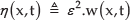
The co-ordinate frames X1Y1 and X2Y2 shown in Fig. 1 are fixed frames, and the xy-frame is a moving coordinate frame which is attached to the beam at its midpoint. Consider a beam of length L and mass m = ρL, where ρ is mass per unit length. The mass centre position and orientation of the beam with respect to X1Y1-frame are given by{c0} = {x0,y0,θ}T. The Z and z directions are perpendicular to the plane. F1x,F1y,F2x,F2y are the forces applied by the manipulator at the two ends of the beam. The transverse displacement η(x,t) is measured with respect to xy-frame and deformation in the longitudinal direction is neglected. All kinematic relations are written with respect to the X1Y1 frame, as shown in Fig. 2. Any point on the beam can be written as,
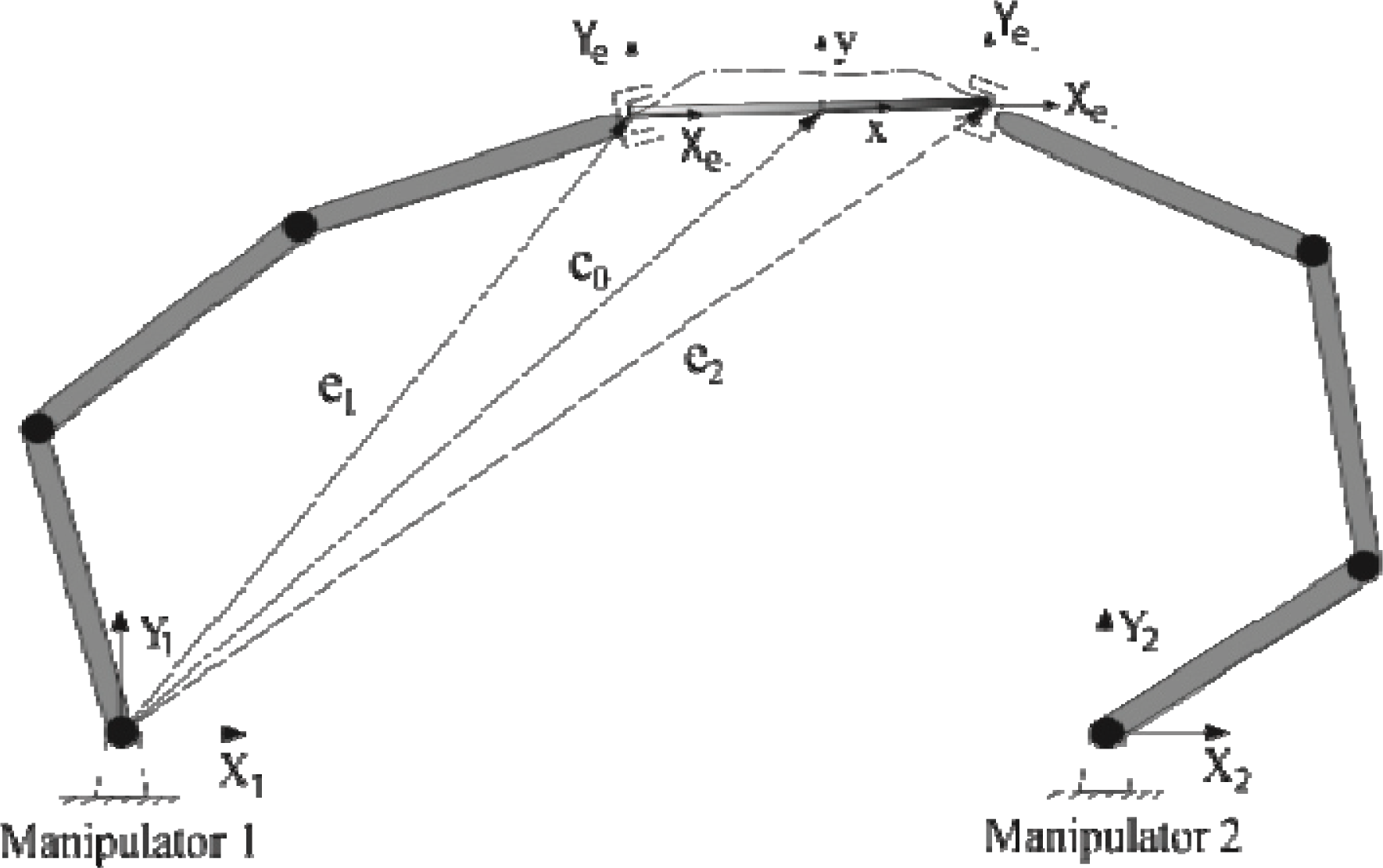
Two planar rigid manipulators grasping a flexible object

Flexible beam with coordinate frames
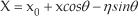

where x is the spatial co-ordinate ranging from
The beam has rigid body motion on which the flexible motion or vibration of the beam is superimposed. It is evident from Fig. 1 that the left and right end point of the beam shares the left and right end-effector grasping point of the two end-effectors. Assuming that the slope due to transverse deflection is negligible compared to the orientation of the beam, the slopes at the two ends of the beam are neglected.
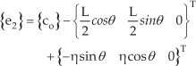
The following relations are obtained from Fig. 2.
The left end pose (position and orientation) of the beam is given by

and the right end pose of the beam is given by
Differentiating (3) and (4) results in

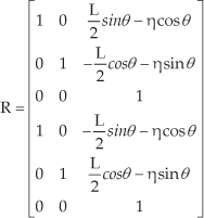
Above relations can be written in compact form with respect to the Cartesian co-ordinates as

where
Differentiating (5) gives the acceleration

where
B. Dynamics of the Beam
In order to determine the dynamic equations of motion of the beam, the kinetic energy, potential energies due to elasticity of the beam and due to gravity must be obtained. Then, by applying the extended Hamilton principle [22], the dynamic equations of the beam will be derived.
Kinetic energy of the beam is defined as

Differentiating (1) and (2) gives


Squaring (8) and (9) and substituting into (7) yields

Neglecting the shear deformation and considering the bending of the beam, the potential energy of the beam due to elasticity can be obtained as

where,

Further, σxx,εxx, dV and E denote the stress, strain component, infinitesimal volume and Young's Modulus of a beam element, respectively. Bending strain is measured at a distance yd from the neutral axis of the beam.
Substituting (12) into (11) gives
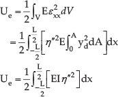
where,
Potential energy due to the gravitational force can be obtained as

Total potential energy can be calculated by the following

Work done due to the external forces (Fig. 2) are formulated as

By applying the extended Hamilton principle,
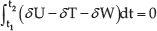
the following equations of rigid motion of the beam along X, Y and Z directions are obtained.
The equation of motion for translation along the X - direction is derived as

The translation in the Y-direction is described by the equation
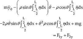
Rotation about the Z axis is described by

The differential equation of motion of transverse vibration of the beam is expressed as

Hence, from (18), (19) and (20) the beam dynamics of the rigid motion with respect to Cartesian coordinates {x0 y0 θ}T can be written in a compact form as


The flexible motion is the transverse vibration of beam dynamics (21) which can be rewritten as

The dynamic equations of the beam have been expressed in (22) and (23). In the following development, the dynamics of two manipulators rigidly grasping the beam will be combined with the beam dynamics (22) and (23) to form complete system dynamics of the manipulators-beam system.
3. Manipulator dynamics and combined dynamics
A. Manipulator Dynamics
The general manipulator dynamic equation can be expressed as [23]

Mi(qi) represents symmetric positive definite inertia matrix, Ci(qi,q̇i)q̇i is the vector due to Coriolis and centrifugal components, Gi (qi) represents the vector of gravitational components, τi is the vector of input torque applied at each joints of the manipulator, fi is the interaction force between the manipulator and the flexible beam, Ji is Jacobian matrix of manipulator, and qi is the vector of joint angles. The two manipulator equations are assembled and can be written in joint space as

where,

It can be seen from (22) that the beam dynamics is represented in Cartesian space and the manipulator dynamics (25) is given in joint space. In order to formulate a complete system of dynamic equations in Cartesian space, the manipulator dynamics will be converted into Cartesian space and the result will be combined with the beam dynamics to form the combined dynamics.
B. Combined Dynamics
The following procedure illustrates the procedure to convert the manipulator dynamics into the Cartesian space and finally to obtain combined dynamics. A well known kinematic relation between the end-effector velocity and joint velocity gives [24]

For the two manipulators

Equation (27) in an assembled form can be written as

where

Substituting (5) into (28) yields

Differentiating (29) gives
For simplicity, parentheses for vectors and square brackets for matrices are omitted in the following.
Substituting (29) and (30) into (25), we obtain the manipulator dynamics in Cartesian space

Premultiplying (31) by RTJ–T gives

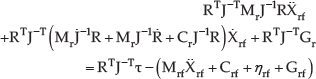
In view of the assumption of simply supported beam boundary conditions, the moments at the two ends are zero. However, in reality manipulators experience forces as well as moments at the two ends of the beam [2]. Utilizing this fact, the moments at the two ends of the beam should be included in the matrix Frf of (22), which results in

In this case, Frf is equivalent to RT. Combining the rigid motion of the beam dynamics (22) with the manipulator dynamics in Cartesian space (32) yields the combined rigid dynamics as
The above combined rigid dynamics can be rewritten as

where,

Taking into account the transverse vibration of beam dynamics, the complete manipulator-beam system dynamics is represented as


4. Singular perturbation model
The control task is stated as follows: for any given desired bounded trajectory of the mass centre of the beam Xrfd and Xrfd, with some or all of the manipulator and beam parameters unknown, derive a controller for the manipulators τ such that the beam centre Xrf tracks Xrfd, while suppressing the vibration of the flexible object, to zero.
The system dynamics derived without using any approximation methods given in (35) and (36) have rigid as well as flexible parameters that are coupled together. To achieve the above control objective for such a complicated nonlinear system, a suitable control approach is the two-time scale theory which considers the high frequency phenomenon of flexible motion in different time scales. The basic idea for the two-time scale theory is to identify the slow and fast subsystems in separate time scales by employing the singular perturbation approach [25]. Then, control algorithms are designed for each of the subsystems, which will be combined to yield the composite control strategy for the original system. However, the challenge is to design the subcontrollers to satisfy the so-called Tikhnov theorem in order to guarantee that the composite controller can be applied to the original system, especially when the parameters of the system are unknown.
Since the manipulators are assumed to be rigid, the corresponding inertia matrix Mr, Coriolis and centrifugal matrix Cr, gravitational vectors Gr and Jacobian matrix J do not have any flexible parameters. The beam has rigid as well as flexible parameters and are coupled together in Mrf, Crf, ηrf and also in R. These flexible parameters have to be uncoupled from the above matrices and vectors by using the singular perturbation technique. This technique also accounts for the neglected high frequency characteristics when the beam undergoes vibration [20]. Using a perturbation parameter, say ε2, the order of the system dynamics can be changed and this small parameter depends upon the system variable. Keeping that in mind, the term EI / ρ in (36), which has large magnitude compared to other coefficients [20], can be redefined as,

where K is a dimensionless parameter which has a large value for the different materials [20] and [25], and its order is equal to EI / ρ and also the variable “a” satisfies the equalities. For example, an aluminium rod with a diameter of 0.05m, E=71 GPa and ρ = 2700kg / m3 has the value of the co-efficient EI / ρ ≅ 4.1 × 10³ and therefore a = 4.1 and K = 103.
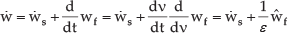
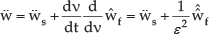
The beam has rigid motion with respect to the state variables Xrf = {x0 y0 θ}T and also the transverse vibration η with respect to the state variable occurs in different time scales. Then, one needs to introduce a new variable w(x,t) in the same order as the state variable by using the following
where ε2 = 1 / K is the so-called perturbed parameter.
Using (38) one can rewrite the rigid motion dynamics of the beam as follows:
The equation of motion (18) in the X-direction can be written in terms of perturbed parameter as

The equation of motion (19) in the Y-direction can be written in terms of perturbed parameters as

Rotation about the Z axis described in the equation of motion (20) can be rewritten in terms of perturbed parameter as

Accordingly, utilizing (37) and (38), the equation of motion for transverse vibration of the beam can be rewritten as

The equations (39), (40), (41) and (42) represent the singularly perturbed form which will be incorporated into the system of dynamic equations (35) and (36) to form the singularly perturbed model of the complete system.
5. Slow and fast subsystems
In this section, the two subsystems, namely slow and fast, are obtained by following the typical steps of the singular perturbation approach. Due to the presence of perturbed parameter ε2, the complete system has two motions in the different time scales. Initially, the singularly perturbed model of rigid motion dynamics of the beam will be converted into the rigid dynamic model without involving any flexible parameter, and finally, it will be incorporated into (35) to form the slow subsystem. Similarly, after following the usual procedure of the singular perturbation approach, the fast subsystem will be obtained from (42).
A. Slow Subsystem
When the perturbation parameter ε approaches zero, the equivalent quasi-steady-state system [26] represents the slow subsystem. By setting ε = 0, (39), (40) and (41) we form the rigid dynamic model of the beam which is given in compact form as


The equation of motion for transverse vibration of the beam (42) becomes

where fs corresponds to f when ε = 0.
Again, substituting (38) into (5) and also setting ε = 0,R becomes R1 which is given by

Based upon the above results, the combined dynamic Equation (35) becomes

where

The above equation can be rewritten as

where

The slow subsystem given in (46) represents the rigid body motion without involving any flexible parameters. It will be used further to design a control algorithm to track a desired trajectory of the object.
The slow subsystem has the following properties which are important to the stability analysis and these properties can be proved.
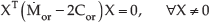
where X is any arbitrary vector. Hence, (Ṁor − 2Cor) is a skew-symmetric matrix.

where Yor ∈
B. Fast Subsystem
Equation (42) represents the perturbed flexible model obtained with perturbation parameter ε which is very small and solely depends upon the E,I and ρ.
In order to study the dynamic behaviour of the fast system, the so-called boundary layer phenomenon [25] and [26] must be obtained. This can be identified by ensuring that the slow variables are kept constant in the fast time scale

Differentiating the fast time scale

Differentiating (49) gives
where ŵf denotes differentiating fast variable with respect to fast time scale.
Differentiating (51) again yields
Utilizing (49), (42) can be rewritten as

Utilizing (44) and (52), (53) becomes

By defining Ff f(ff) = Ff f(f) – Ff f(fs), the above equation can be rewritten as

However, in the boundary layer system, the slow variable ws is constant which implies ẅ = 0 and also ε = 0 [26]. Then, the fast dynamics can be represented as

Following [19] and [27], an operator A is defined as

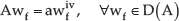
where, D(A) denotes the domain of the operator A and H denotes the Hilbert space. The operator A has the eigenvalues λi and the corresponding eigenfunctions ϕi satisfying the following conditions [27].
0 < λ1 < λ2 ……, limλi = ∞ Aϕi = λiϕi, i = 1, 2….∞ The set of the eigenfunctions forms a complete orthonormal system in the Hilbert space.
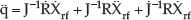
Utilizing (58), the partial differential Equation (56) can be rewritten as an abstract differential equation on H as

Equation (59) represents the fast subsystem which will be used for designing fast feedback control.
6. Composite control
A composite control for the two manipulators and beam system is given by

where us is designed based on slow subsystem (46) and uf is designed to stabilize the fast subsystem (59).
A. Robust Controller Design for Slow Subsystem
The key issue is that with the unknown manipulator and beam parameters, the design of us(Ẋrf,Xrf,t) cannot be arbitrary. It has to guarantee the exponential tracking of the desired trajectories so that Tikhnov's theorem can be satisfied, which will be clear in the later development. For that purpose, a sliding mode control approach will be adopted.
Define the tracking error as

where Xrfd is the desired trajectory and the auxiliary trajectory can also be defined as

where λ is a positive definite matrix whose eigenvalues are strictly in the right half of the complex plane.
The sliding surface can be chosen as

The sliding mode controller can be given as

where KD is a positive definite gain matrix,

where Γ ≥ ‖αor‖ fall is the upperbound of αor which is known though it could be conservatively selected.
B. Control Design for Fast Subsystem
The objective of the controller is to suppress the vibration of the flexible object by incorporating the following feedback control law
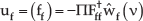
where Fff† can be found using pseudo inverse. The operator ∏# is neither self-adjoint nor positive definite, and it is also shown in [19] and [28] that it is A-symmetric and A- positive semi-definite. This operator was formulated in [28] as Π = kQA, where Q is a bounded and positive definite operator. In addition, the velocity signal ŵf (v) can be measured using a velocity sensor. It is to be noted that there are some established results available using the velocity feedback, for example in [29] and [30]. However, they have considered the assumed modes where, as in the present control algorithm, no form of approximation is used. Additionally, the recent boundary control methods available in the literature [20] and [21], utilizes velocity and slope of fast state variables as feedback which depends upon the boundary conditions of the beam. However, the present control algorithm uses only velocity as feedback which is irrespective of boundary conditions. This controller is simple to implement in real time and needs only a limited number of sensors.
Substituting (65) into (59) gives a closed loop system defined by

Utilizing the operators Π and Q, (66) can be rewritten as

where k is the positive gain and the term QAŵf(v)is the special damping term [28]. This damping has been studied by various researchers especially [31]-[34]. The two operators Q and A are related by Q = A
β
and β varies between
C. Stability Analysis
Tikhnov's theorem [35] is used to justify a composite control strategy that uses a fast feedback control to stabilize the fast subsystem together with a slow control based on a slow subsystem. Tikhnov's theorem basically states the following with regard to the complete manipulators-flexible beam system under the composite control.
If the slow subsystem in (46) is exponentially stable defined on an interval [t0, ∞] and the boundary-layer system or fast subsystem in (59) tends to be also exponentially stable, uniformly in [t, slow variables], then there exists ε* such that for all ε < ε*
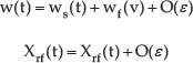
holds uniformly for t ∈ [t0, ∞], where O(ε) ≃ w(t,ε) – ws(t), represents the order of the error which arises due to the difference of the original variable w starting at t0 from a prescribed initial conditions δ(ε) and the quasi-steady state variable ws is not free to start from a prescribed initial value. There can be a discrepancy between its initial value and already prescribed initial value which causes this order of error. It will be hold in the interval excluding t0 that is, for t ∈ [tb, t1] where tb > t0.
1) Exponential Stability of Slow Subsystem: Tikhnov's theorem requires the slow subsystem to be exponentially stable. The following derivation will illustrate the exponential stability of the slow subsystem for all t > 0. . Differentiating the sliding surface (62) with respect to time. Gives

multiplying both sides of (68) by Mor and using (46), (68) can be rewritten as

Adding and subtracting CorX̄r in (69) results in

Using (62), (70) can be rewritten as

where

Consider a Lyapunov function candidate as

Differentiating (73) with respect to time gives

Substituting (71) into (74) and also using property 2 given in (47), the above equation yields

Substituting the control law given in (63) and (64) into (75) results in

Taking transpose of ‖STYor‖ and also Γ ≥ ‖αor‖ gives
It is known that [36] KD = M0rκ, where κ can be considered as a least eigenvalue. Hence, (77) can be rewritten as

Using (73), (78) can be rewritten as

The solution of above equation is

It is evident from the above equation that the sliding surface will converge exponentially to zero. Thus the sliding surface is related to the tracking error er in (62) which also converges exponentially to zero which satisfies Tikhnov's theorem.
2) Exponential Stability of Fast Subsystem: Tikhnov's theorem requires that the fast subsystem must also be exponentially stable. The energy multiplier method used in [28] is followed to prove the exponential stability under the following theorem [37], [theorem 4.1] which guarantees exponential stability.
then there are constants M ≥ 1 and μ > 0 such that ‖T(t)‖‖ ≤ Me–μt
Note: It is also shown in [28] and [38] that the property of Lp stability and exponential stability for a strongly continuous semigroup must satisfy the following

where E(v) is weakly monotonically decreasing function with respect to fast time scale v [38]. The fast time scale derivative of E(v) from the above equation will be

Let us choose 0 < ε < 1 and the Lyapunov function candidate is given by

We have the following relation

There exists a constant C1 such that

For v > v1 the Lyapunov function is positive and v1 is from

The derivative of V2(v) with respect to the fast time scale is given by

For any arbitrary constant, say, C2 > 0 we have

Using (89), (88) can be rewritten as

where
If C2 can be chosen as large then

where v2 can be

The above result in (91) shows that derivative of Lyapunov function has a decreasing nature for v > v2, and it is also evident from (84) that the energy will also be dissipating for v > 0. Using these facts, for v > T ≔ max{v1,v2} and also from (86) E(v) can be estimated as

Then, (92) can be rewritten as

which confirms the exponential stability as given in (81) and hence it is proved.
By choosing the appropriate Lyapunov function candidate for the slow and fast subsystems, stability analysis has been carried out. It is evident from the above analysis that both the systems converge to zero exponentially which satisfies Tikhnov's theorem. Therefore, by using this composite control strategy, the flexible object will track the desired trajectory and simultaneously suppress the vibration.
Since the control law (63) and (64) is discontinuous across the sliding surface, such a control law leads to chattering. Chattering is undesirable in practice because it involves high control activity. To remedy this drawback, it usually uses
where Γ becomes
7. Simulation studies
In the simulation, two identical planar rigid manipulators, each with three-links/revolute joints, are used to move the flexible beam along a desired trajectory specified by,

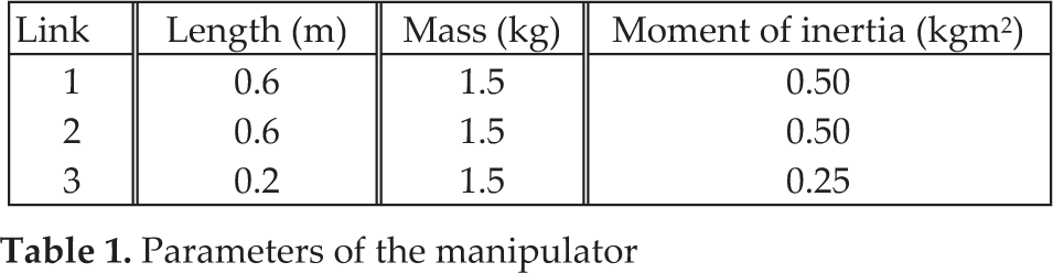
The parameters of the identical manipulators [40] are given in Table I and the flexible beam parameters are given in Table II.
Parameters of the manipulator
Parameters of the flexible beam

The beam initial position and orientation are Xrf = {0.51m,0.36m,0.1rad}T and initial velocity and acceleration are considered to be zero. Initial joint angles of manipulator are q11 = 0.2974 rad, q12 = 1.6974 rad, q13 = −1.6948 rad, q21 = 0.2149 rad, q22 = 1.4886 rad and q23 = −1.4306 rad, respectively. The initial joint velocities of all the joints of manipulators are 0.001 rad/sec and joint accelerations are assumed to be zero. The simulation was carried out with a sampling period of 0.01 sec. The control parameters are given in Table III. The value of Γ was chosen based on the L∞ norm of the time independent parameters of the regressor and in this case, vector αor.
Control parameters

The regressor for the slow subsystem is very lengthy and due to space limitations it is not provided but can be made available upon request. Figs. 3 and 4 show the tracking of the planar motion of centre of the object along X, Y-directions. The orientation of the beam is shown in Fig. 5 and also the tracking error is shown in Fig. 6. It can be observed that the tracking of position and orientation is achieved within 1 sec, which shows the effectiveness of the controller. In order to achieve the desired trajectory of the object, both joints of the manipulators are moved in a smooth manner which are shown in Figs. 7 to 12. The sliding variables are shown in Fig. 13.

X-position tracking

Y-position tracking
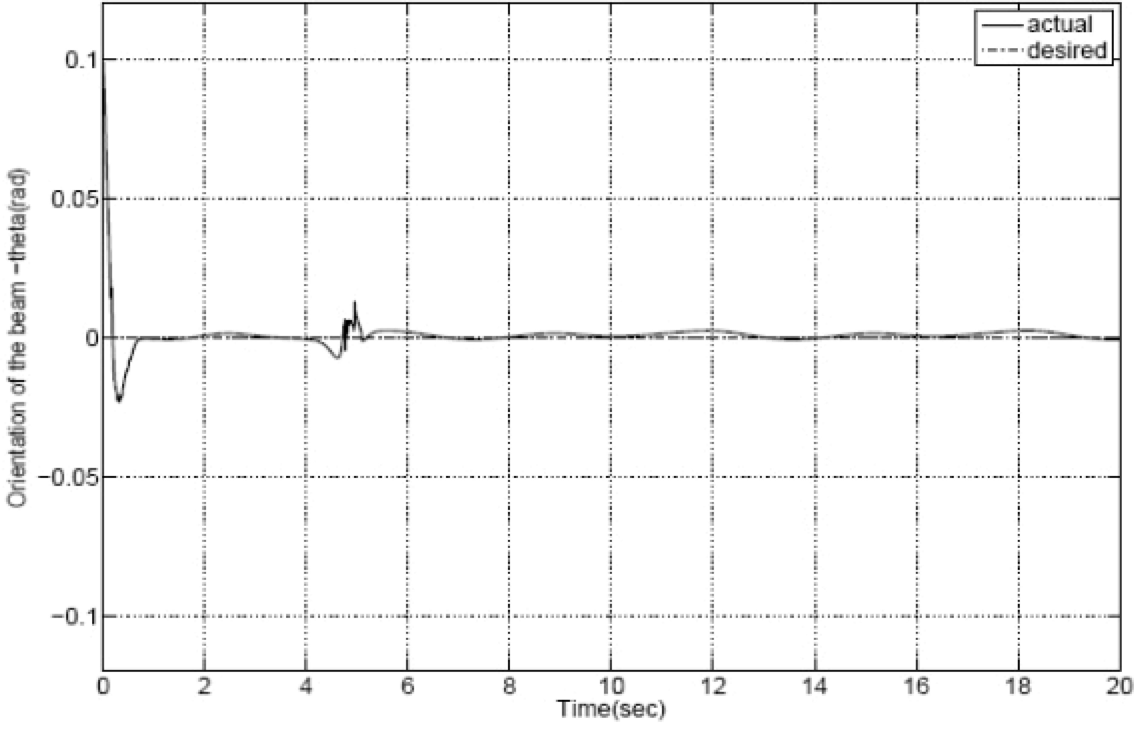
Orientation of the beam

Tracking error

Angular motion of joint 1 of manipulator 1

Angular motion of joint 2 of manipulator 1

Angular motion of joint 3 of manipulator 1

Angular motion of joint 1 of manipulator 2

Angular motion of joint 2 of manipulator 2
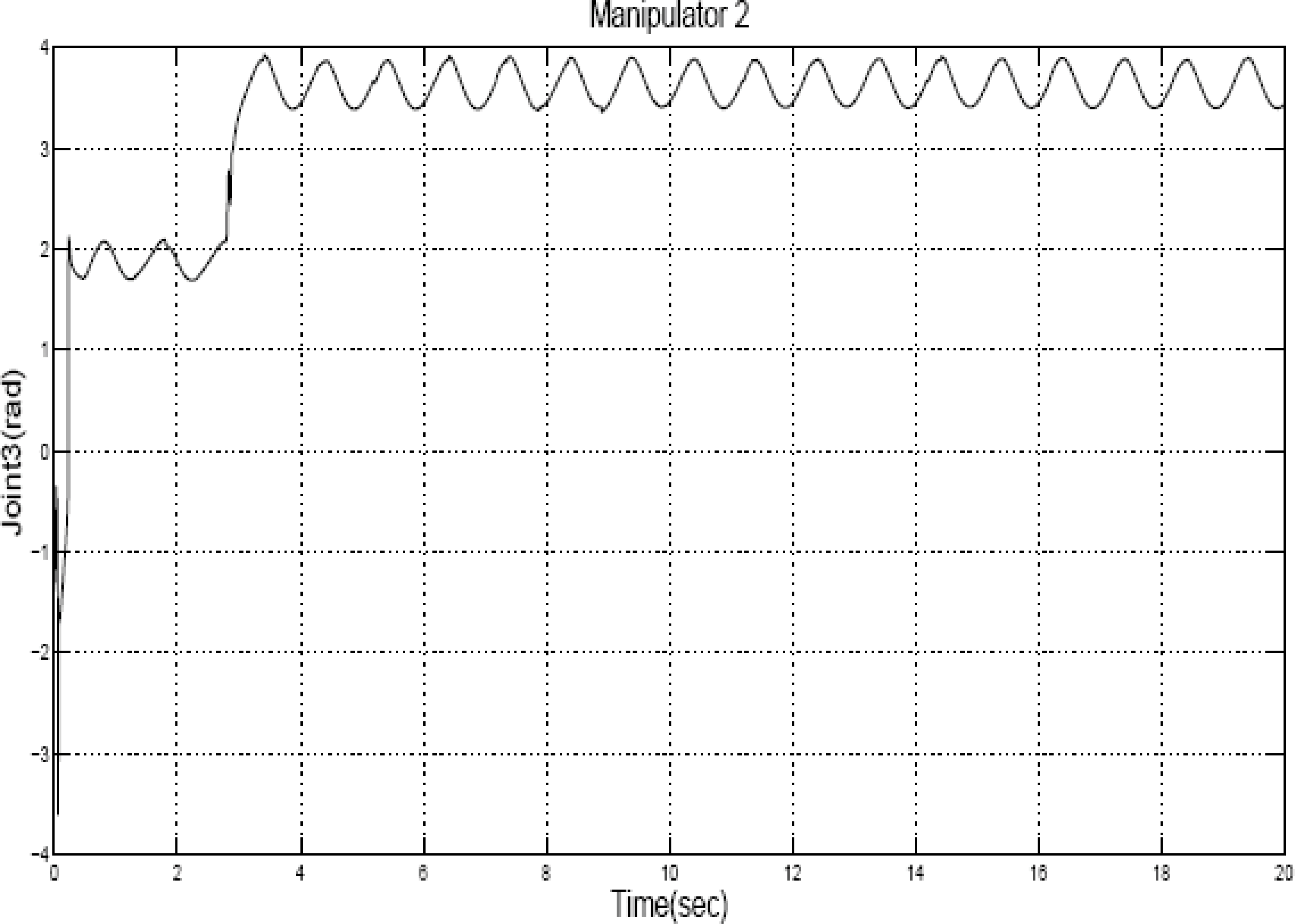
Angular motion of joint 3 of manipulator 2

Sliding variables
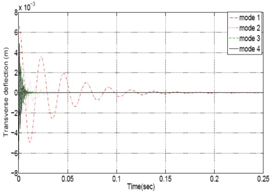
In the case of fast subsystem, the initial disturbance of 5 mm with zero initial velocity is considered for the simulation. Although, the beam dynamic equation is not assumed with the number of modes, simulation has to be performed with the assumption of modes. Normally, only the first few modes are dominant, yielding a higher vibration response and hence the first four modes are considered here. For the case of structural damping characteristics when β = −0.5, in Fig. 14, the vibration yields oscillatory motion that is completely suppressed at around 1 sec. It is also shown in Fig. 15 that exponential decay occurs at β = 0 which corresponds to the overdamping behaviour of the fast subsystem which is same for all modes. Simulations are also carried out for different damping ratios of 0.1 and 0.4. The results in Figs. 16 and 17 show that with an increasing damping ratio, the amplitude of vibration is significantly suppressed. Furthermore, the transverse displacement under the simply supported end condition of the beam with a damping ratio of 0.1 is evaluated at various locations of the beam using the modal summation method. Due to the symmetry of the boundary conditions, the deflection at 0.1 m from the left end and at the middle of the beam are considered. It can be seen from the Figs. 18 and 19 that the centre of the beam yields more deflection than any other point of the beam.
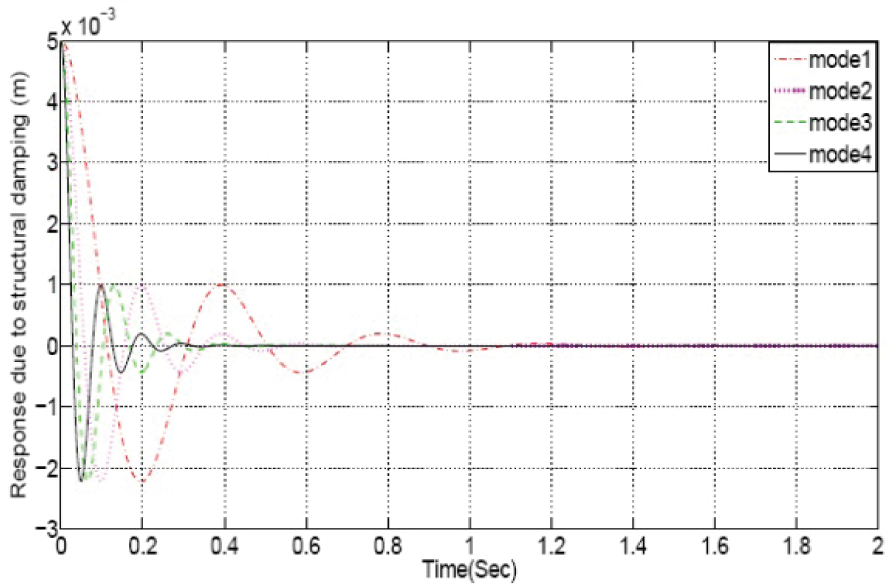
Structural damping characteristics β=−0.5
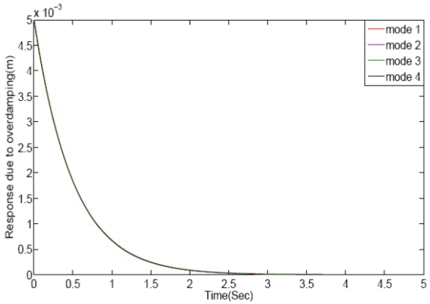
Strong damping characteristics β= 0
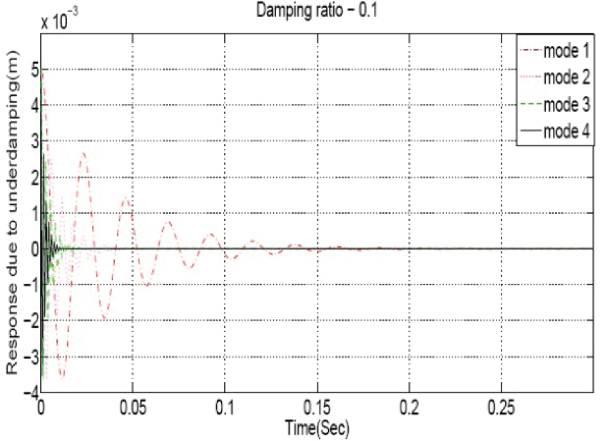
Deflection of the beam for damping ratio=0.1
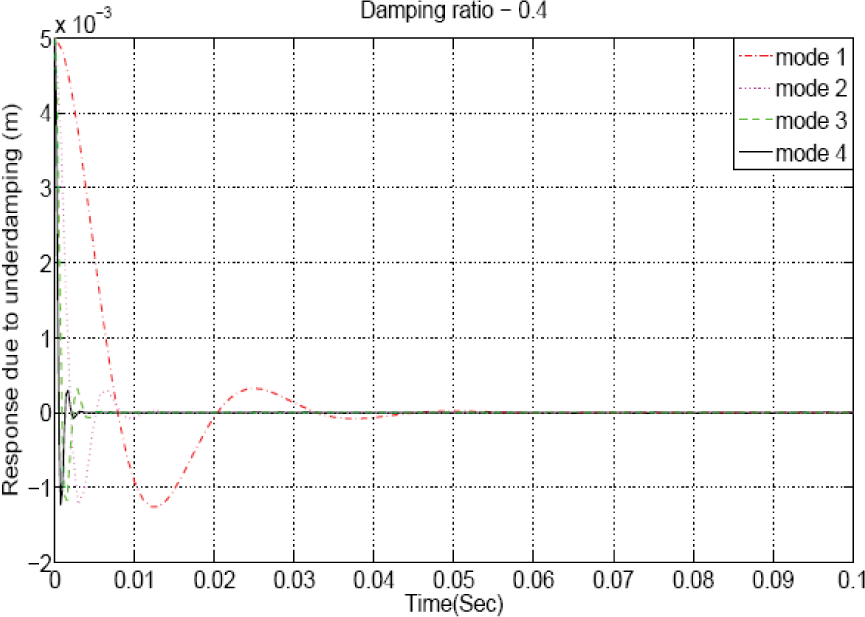
Deflection of the beam for damping ratio=0.4

Deflection at 0.1 m from the left end of the beam
Deflection at mid point of the beam
Simulations were carried out with different masses of the beam and the results are shown in Figs. 20 and 21. It can be seen that the response is higher for lower masses. Results are also presented for different lengths of the beam in Figs. 22 and 23. It is seen that the responses are higher for longer beams.

Mass of the beam 2 kg

Mass of the beam 5 kg

Length of Beam 1 m
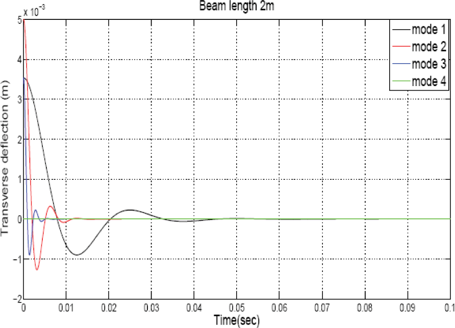
Length of Beam 2 m
8. Conclusion
In this article, the problem of two planar rigid manipulators used to move a flexible object along the desired trajectory while suppressing the vibration of the flexible object is considered. The kinematic and dynamic relations of the beam are derived without either approximating or discretizing the beam.
The complete system is then obtained by combining both the dynamics of the beam and the manipulators. To control this highly nonlinear system, the singular perturbation method is adopted, where the slow and fast subsystems are separately obtained. Based on Tikhnov's theorem, a regressor-based sliding mode control algorithm is designed for the slow subsystem, and a simple feedback control law is selected for the fast subsystem to form a composite controller. The simulation results show that the proposed composite controller is an efficient choice in tracking the desired trajectory while suppressing the vibration of the flexible object.