
Abstract
In this paper, a new motion controller for a quadrotor aircraft is introduced. A reformulation of the control inputs of the dynamic model is discussed and then the control algorithm is given in a constructive form. The stability proof of the state space origin of the overall closed-loop system relies on the theory of singularly perturbed systems. Numerical simulations corroborate the viability of the proposed control scheme and the conclusions concerning stability. A set of simulations under practical conditions is also presented, where the system is affected by different types of disturbances and nonlinearities such as noise and actuator saturation.
Keywords
1. Introduction
The study of the design and applications of unmanned aerial vehicles (UAVs) has been an important topic over the last few years. The current and potential applications of these vehicles are extensive, such as surveillance, rescue, espionage and entertainment, to mention a few.
UAVs can be controlled automatically to track a flight plan. From the theoretical point of view, UAVs are quite challenging since in most cases they are underactuated systems, which means that these systems have more degrees-of-freedom than control inputs.
The quadrotor is an UAV with six degrees-of-freedom and only four control inputs (four rotors). The control of the quadrotor is difficult because the nonlinearity of its dynamic model [1]. It is not possible to control all of the states at the same time. However, one can select some states to be controlled. A possible combination of controlled outputs can be the translational position and the yaw angle. The roll and the pitch angles can be controlled indirectly by introducing stable zero dynamics [2], [3].
Many methods to achieve attitude stabilization and trajectory tracking control have been proposed in recent years. In [4], the authors proposed a partial state backstepping sliding mode controller using a simplified model of the quadrotor. In [5] and [6], the application of the backstepping methodology to the control of quadrotors was revisited, showing that motion control can be achieve within the Lyapunov function framework. In [2], [3] and [7], a visual feedback is added to achieve stabilization of the system at the desired configuration. An experimental evaluation of a control approach was discussed in [8]. The work introduced in [9] proposed a neural network controller for the robust trajectory tracking control of the quadrotor posture. It is assumed that the model is partially known and that the system is subject to wind disturbances. By using the Newton-Euler formalism, a backstepping-based controller was introduced in [10]. [11], the feedback linearization technique is used to derive a tracking controller. An analysis of the internal dynamics is included in that work. More recently, in
[12], a modified sliding mode term is designed with the aim of controlling the attitude of a quadrotor aircraft subject to a class of disturbances. A motion controller composed of six nonlinear PD loops is introduced in
[13]. The controller guarantees that the error trajectories are uniformly bounded. The design of a controller based on the block control technique combined with the super twisting control algorithm for trajectory tracking of a quadrotor aircraft is introduced in [14].
The recent textbooks [15] and [16] can be consulted for further references on the history, modelling, motion planning and control of quadrotors.
Control approaches, such as feedback linearization, backstepping, sliding modes, adaptive control, to mention a few, match the idea that the resulting closed-loop system should satisfy Lyapunov's theory. As an alternative, the theory of singularly perturbed systems has also been recognized as a powerful tool in the analysis and design of controllers for different kinds of systems such as electromechanical, biological and electrical, see for example [17] and [22]. Essentially, this technique is based on analysing the convergence of the solution of a set of differential equations in two (or more) time scales.
Recent applications of the theory of singularly perturbed systems in the derivation of controllers for mechatronic systems can be found in [18], [19], [20] and [21]. The derivation of the controllers only considered the existence of gains assuring the time scale separation while numerical simulations and real-time experiments confirmed their practical viability.
The theory of singularly perturbed systems is well-adapted to the design of trajectory tracking controllers for quadrotor systems, since control laws can be easily synthesized by using different time scales. The error dynamics obtained by using a controller inspired from time scale separation should satisfy a set of conditions to guarantee that the error trajectories really converge to zero as time increases. The theory of singularly perturbed systems established in [17] provides a rigorous framework to prove the convergence of systems with different time scales.
In the next section, references about control designs for quadrotors inspired in time scale separation are provided.
A motion controller was proposed by Zuo [23], which is based on using a new command-filtered backstepping technique to stabilize the attitude and a linear tracking differentiator to eliminate the classical inner/outer-loop structure. The work by Bertrand et al. [24] deals with the regulation problem and the time scale separation by introducing an angular velocity controller in terms of a perturbing parameter together with the angular velocity commands. Esteban et al. [25] propose a control scheme for a radio-controlled helicopter. Stability proof is based on using a three time scale separation.
The design of control algorithms for quadrotor aircraft which ensures tracking of a desired time-varying trajectory via the theory of singularly perturbed systems still requires study since literature related to these subjects is limited.
In this document, a new control algorithm is introduced. The proposed controller has been derived by using the following time scale separation ideas:
Differential equations with fast time scale are generated by using an angular proportional-integral velocity controller.
Differential equations with medium time scale are generated by a kinematic-like scheme, which generates angular position commands.
Differential equations with slow time scale are generated by the translational position controller. The translational dynamics is controlled indirectly by designing proper orientation commands. As seen later, those commands are designed under the assumption that the angular position is null.
An advantage of the proposed scheme is the addition of integral action, which is helpful in compensating model uncertainties and external disturbances. The overall closed-loop system stability is studied rigorously by using the Lyapunov theory and stability of singularly perturbed systems [17].
The present document is organized as follows. Section 2 is devoted to the quadrotor dynamics and the control goal. The proposed motion control algorithm is described in Section 3. Section 4 provides the proof that the state space origin of the resulting closed-loop system is exponentially stable. Section 5 describes the simulation results, which have the purpose of confirming that by using the proposed scheme the quadrotor matches exponentially a desired translation chaotic trajectory and a desired periodic yaw angle.
Simulations considering that the system is affected by perturbations and nonlinearities that appear in a practical implementation are provided in Section 6. There, the time scale separation introduced by the proposed controller is also confirmed. Additionally, Section 6 presents the results by using a desired translational helicoidal trajectory.
Finally, some concluding remarks and discussion on further research are provided in Section 7.
2. Quadrotor dynamics and control goal
2.1. Quadrotor dynamics
The equations of motion of the quadrotor are studied in the recent textbooks [27], [16] and [15]. The quadrotor dynamics is represented by a set of six ordinary differential equations of second order. In order to represent the quadrotor dynamics, we have used three differential equations derived in the inertial frame and three differential equations derived in the body frame. The inertial frame is denoted by
However, as discussed in [23], [28], [30], [31], [32] and [33], the quadrotor dynamics can also be represented by using three equations for the translation dynamics obtained in the inertial frame

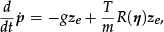

where the constant m is the mass of the quadrotor, g is gravity acceleration,

is a unitary vector in the z direction of the inertial frame which is used for compactness of the notation,
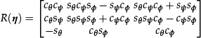
is an orthogonal rotation matrix that describes a clockwise/left-handed rotation with x-y-z convention, the lift forces fi generated by the four propellers can be arranged in the vector
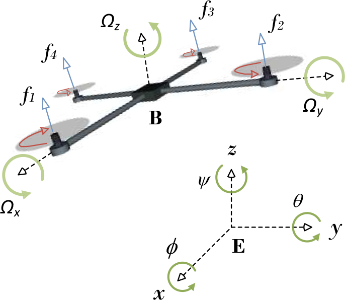
The quadrotor aircraft and reference frames

which will be considered the control input,

is the total thrust and the vector
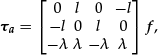
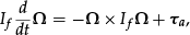
represents the torques applied to the quadrotor, which are generated by the lift forces of the rotor propellers.
Additionally, concerning the equation (3),

In order to guarantee the non singularity of W(
Notice that the relationship (3) from angular velocity in the body frame

where

Throughout this paper the vector
2.2. Control problem formulation
Considering the vectors

is the orientation error and

is the Cartesian position error.
Roughly speaking, the control problem consists in designing a control algorithm

is guaranteed for a compact set of initial conditions of the quadrotor state variables.
As will be seen later, the specification of the desired position pd(t) should be differentiable at least up to order four and the desired angular position ηd(t) should be differentiable at least up to order two, while the desired roll angle φd(t) and desired pitch angle θd(t) should introduce stable position error dynamics, with the angle specification of the desired yaw ψd(t) assumed to be at least twice differentiable.
3. Development of the proposed algorithm
The proposed controller

where

Matrix B(

which is singular for
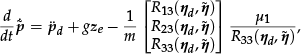
The matrix B(

where µ1 is the first element of the vector
By developing the calculations, the proof of property (11) is obtained.
By using property (11) it is possible to show that under the control law (9) the quadrotor dynamics (1)–(4) becomes


where µ1 ∈ ℝ is the first component of
The block diagram implementation of the proposed controller can be appreciated in the Figure 2. As will be seen in the next section, the proposed scheme has an inner loop of angular velocity control and an outer loop of translational and angular position control.
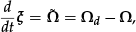
3.1. Control of the angular dynamics
We solve the problem by using the following controller

where the Kpw and Kiw are 3×3 positive definite matrices. It should be noted that this control structure matches the PI velocity controller for the robot manipulators reported in [35], which is adapted from the structure of the well-known PD+ motion controller [34]. The addition of integral action has the advantage of improving the rejection of time-varying disturbances and model uncertainties.
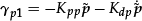
To guarantee that the actual orientation

with Kpo a 3 × 3 symmetric positive definite matrix.
Thus, the angular error dynamics is given by


The only equilibrium point of system (19)–(21) is given at the state space origin, that is,


Block diagram of the proposed motion control algorithm which is based on a primary model-based angular velocity tracking controller and secondary kinematic-like translational and angular position controller.
3.2. Control of the translational dynamics
By using the definition of

Now, in order to design a way to stabilize exponentially the system (22)-(23), let us assume that

Assumption (24) will be relaxed later when the stability analysis is presented. It is clear that in practice, either asymptotical or exponential tracking of the desired angular position
Invoking assumption (24), the translational error dynamics (22)-(23) becomes


where the d subscript in Rijd means that the signal Rij depends on

It is worth noticing that
If the desired Euler angles are specified so that equation (27) is satisfied, the translational error dynamics (25)-(26) is then given by


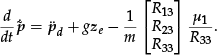
Therefore, the selection of the PD structure
stabilizes exponentially the translational error dynamics (28)-(29).
Let us rewrite equation (27) as

where


where γ11, γ12 and γ13 are obtained from (31).
Notice that the computation of

At the same time, the calculation of
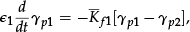
In order to respect the assumption that the only measured signals are those of the state


where Kf1 and Kf2 are 3 × 3 symmetric positive definite matrices. Thus, the larger the numerical value of Kf1 and Kf2, the faster the convergence of the signal
The explicit definition of
The rest of this section is devoted to explaining the steps to be followed in order to implement the proposed motion controller.
3.3. Summary of the control algorithm
Next, we provide a summary of the equations to implement the proposed trajectory tracking controller. Specifically, we provide the steps to achieve a program for numerical simulation purposes.
In the next section, a theoretical framework for the exponential stability of the overall closed-loop system is provided. Firstly, the closed-loop system is obtained and then stability will be discussed by using the theory of singularly perturbed systems [17].
4. Overall closed-loop system stability via three time scale
Consider the following parametrization of the control gains


and

where ε1 and ε2 are positive constants denoted as perturbing parameters, which satisfy

Therefore, it is possible to show that the overall closed-loop system can be written as


where, by virtue of the angular velocity error
The overall closed-loop system (41)–(47) has the standard form of a singularly perturbed system with a three time scale, which has been conveniently derived through the parametrization of the controller gains (37)–(39).
The stability proof of the system (41)–(47) and the obtention of the time scales are based on the following steps:
The first step in the stability proof, by assumption (40), is the separation of the system in a twofold time scale. Thus,

are the slow states with respect to

which at the same time represents the states with fast time scale.
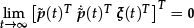
For the second step, exponential convergence of the solutions

are slow states with respect to

Thus, we have that xs represents the states with slow time scale,
Proof: The proof of Proposition 1 is achieved by verifying the conditions of the theorem 9.3 in [17]. The proof of Proposition 1 is set down in the following five items:


with


It is noteworthy that the isolated root (49) evaluated in (31)–(33) gives the specific value


As previously mentioned, the states

are slow with respect to
The local exponential stability of the state space origin of the slow dynamics (41)–(44) can be derived by using again a time scale approach, interpreting

is defined. Let us remember that
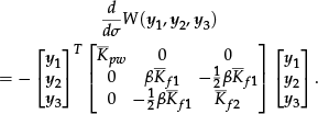
By deriving


which is a linear system. The Lyapunov function for system (55)–(57) is defined as

whose derivative with respect to the fast time scale σ is given by
By invoking Sylvester's theorem, the condition
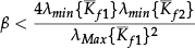
guarantees the inequality

Therefore, because (55)–(57) is a linear system, we have sufficient conditions to claim that there is an arbitrarily large compact set Bρ such that

implies that

as the scaled time σ → ∞.
By theorem 9.3 [17], there are sufficient conditions to claim that there exists ε*1 such that ε*1 > ε1 > 0 guarantees that there is an arbitrarily large compact set RA of initial conditions where the trajectories of the overall closed-loop system (41)–(47) achieves the following limit

The result stated in Proposition 1 means that the goal (8) holds by using the control algorithms in Section 3.3.
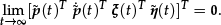
The proof of Proposition 1 is based on the assumption of the local exponential convergence of the slow dynamics (51)–(54). In order to relax such an assumption, the explicit proof of exponential convergence of the slow time states
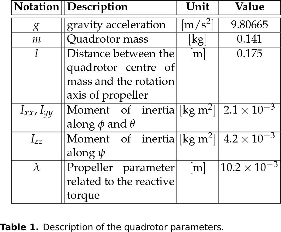
Description of the quadrotor parameters.

Actual quadrotor path
Proof: The proof of Proposition 2 is achieved by verifying the conditions of the theorem 9.3 in [17]. The proof of Proposition 2 is set down in the following five items:

is given by the isolated root


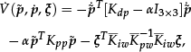
Let us consider the Lyapunov function

with α > 0 small enough so that

The time derivative of
The right-hand side of equation (63) is globally negative definite for a small enough α > 0. Finally, it is possible to prove that the inequality

with some κ2 > 0, is satisfied for all
with exponential convergence rate as time t increases.

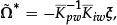
with respect to scaled time ᾱ = t/ε2 and setting ε2 = 0 in (54), the following boundary layer system is obtained:

which is exponentially stable for all K̄po >
By theorem 9.3 [17], there are sufficient conditions to claim that there exists ε*2 such that ε*2 > ε2 > 0 guarantees that there is an arbitrarily large compact set RB of initial conditions where
An interpretation of the results established in Proposition 1 and 2 is the existence of control gains (37)–(39) so as the local exponential stability of the closed-loop (41)–(47) is assured. Additionally, Proposition 1 and 2 guarantee the existence of perturbing parameters ε1 and ε2 such that

which can be used as a tuning guideline.


5. Simulation results
We have used the Matlab and Simulink toolboxes to implement the system described in Figure 1. In the simulations we considered that the initial conditions of the quadrotor and the controller are null. The parameters of the quadrotor are given in Table 1.
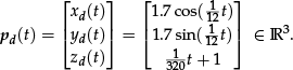
The desired position is defined as

where x̂(t), ŷ(t), ẑ(t), are obtained by means of the Rabinovich-Fabrikant equations [36], that is,

being γ = 0.1 y α = 0.3. Besides,
The desired yaw angle ψd(t) is defined as the time-periodic function

with τ1 = 30 [sec], τ2 = 4 [sec], a1 = 0.5 [rad] and a2 = 0.1 [rad].
Control gains have been selected using the parametrization (37)-(38) and (39). In particular,
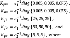

and

On the other hand, the gains of the translational controller are given by

The purpose of the numerical simulations is to confirm that the actual quadrotor trajectories


Time evolution of the norm of the slow time scale states ‖x̄(t)‖, the norm of the medium time scale states ‖z̄(t)‖ and the norm of the fast time scale states ‖y(t)‖ for the different values of the perturbing parameters ε1 and ε2.
the medium time scale states

and the fast time scale states

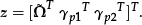
where the quasi-steady-state solution

More specifically, the fast states are
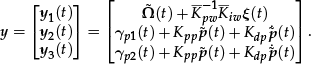
Figure 3 shows the actual quadrotor path
The rest of the Figures show the response of the system for the different values of the perturbation parameters ε1 and ε2. In particular, a simulation has been performed for each combination of the perturbing parameters (ε1, ε2), which gives a total of 20 simulations.
These simulations have been carried out in two nested “for” loops. Each iteration corresponds to a simulation with a combination of parameters (ε1, ε2). In the outer “for” loop, the parameter ε1 is increased and in the inner “for” loop, the parameter ε2 is increased as (69) and (70), respectively. The results are shown in different coloured lines. For each colour, lighter lines mean the former simulations and darker lines mean the latter simulations.
Figure 4 depicts the slow time scale states, given by position errors
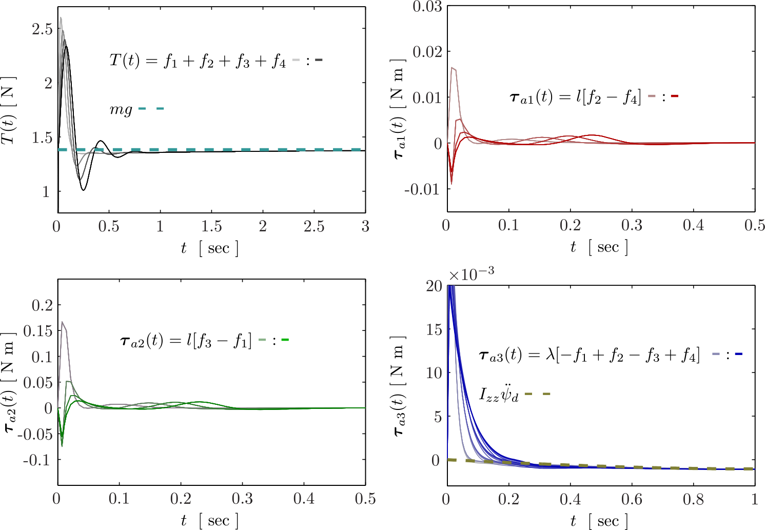
Total applied force T(t) and applied torque

Block diagram of the simulations with practical disturbances.
In Figure 5, the time evolution of the states with fast time scale
Figure 6 shows the time evolution of the norm of the slow time scale states ‖
The results in Figures 4, 5 and 6 confirm that the perturbation parameter ε2 has more effect on the convergence of the medium time scale states, while the perturbing parameter ε1 causes the signal
Finally, the total applied force T(t) and the applied torque τa(t) for the different values of the parameters ε1 and ε2 are depicted in Figure 7. It is appreciated that both signals are well-behaved for all time.
6. Simulations with practical disturbances
Simulations have been carried out incorporating the effect of practical disturbances. In Figure 8, a block diagram showing the incorporation of disturbances in the simulations is provided. The blocks are described as follows:
The maximum amplitude of the noise in the translational displacement is 0.01 [m]. Similarly, the maximum amplitude of the noise in the angular displacement is 0.05 [rad]. Additionally, the amplitudes of the noise added to the time derivative of the translational displacement and angular displacement are 1.0 [m/sec] and 5.0 [rad/sec], respectively.

Under the conditions described above, two different translational position trajectories have been numerically simulated:
The first one corresponds to the equations described by the Rabinovich-Fabrikant system in (65)-(66).
The second one is the helicoidal position trajectory which is usually found in the literature and described by
The purpose of using a chaotic-type desired position trajectory as the one in (65)-(66) is to assess the performance for a flight with acrobatic characteristics. The desired yaw angle ψd(t) specified for the simulations with disturbances is given in (67).
The gains used in the simulations are in (68)–(71). The different values of the perturbing parameters ε1 and ε2 in (69) and (70), respectively, were used to prove numerically the threefold time scale separation.
Figure 9 depicts the actual path
The purpose of showing the velocity signals ‖
By using both types of desired position trajectory
From Figure 10 it can be appreciated that for ε1 = 0.25 and any value of ε2 the signal ‖
The left hand-side plots of Figure 11 describe the forces fi(t) generated by the propellers for the chaotic-type desired position trajectory

Left hand-side plots correspond to the results for the chaotic-type trajectory in (65)-(66). Right hand-side plots show the results for the helicoidal trajectory in (72). The position error
The numerical results shown in Figures 9, 10 and 11 allowed verifying that the threefold time scaling is still present in spite of the fact that practical disturbances are affecting the overall closed-loop system.
7. Concluding remarks and further research
The proposed trajectory tracking controller allows choosing any desired translational position
The overall closed-loop system stability is proven by using the framework of the theory of singularly perturbed systems. This analysis suggested that by using high-gain angular velocity control, the coupling between the translational error dynamics and the angular error dynamics is diminished.
Numerical simulations confirmed that the motion control objective is satisfied with the proposed scheme. In addition, the different time scales introduced by the controller were numerically verified under ideal conditions and under the situation that the system is affected by different types of perturbations that appear in a practical implementation.
A possible disadvantage of the proposed approach is the use of Euler angles to represent the orientation dynamics in equations (14)-(15), which implies that the matrix W(

Left hand-side plots correspond to the results for the chaotic-type trajectory in (65)-(66). Right hand-side plots show the results for the helicoidal trajectory in (72). Using different combinations of the parameters ε1 and ε2, the plots show the time evolution of the forces
Another problem that is left for further research is the estimation of ε1 and ε2 in Proposition 1 and 2, respectively, which can achieved by using a Lyapunov function.
Footnotes
Appendix: Explicit Expression of φ ̇ d,φ ̈ d,θ ̇ d,and θ ̈ d
By using the property
and noticing that
let us first rewrite ηd in the form
By using
the desired angular position becomes
Thus, φd and θd have the structure
whose first time derivative is
and second time derivative is
where
with
and