Sage Journals: Discover world-class research

Abstract

In this paper the authors present three methods to detect the position and orientation of an observer, such as a mobile robot, with respect to a corridor wall. They use an inexpensive sensor to spread a wide ultrasonic beam. The sensor is rotated by means of an accurate servomotor in order to propagate ultrasonic waves towards a regular wall. Whatever the wall material may be the scanning surface appears to be an acoustic reflector as a consequence of low air impedance. The realized device is able to give distance information in each motor position and thus permits the derivation of a set of points as a ray trace-scanner. The dataset contains points lying on a circular arc and relating to strong returns. Three different approaches are herein considered to estimate both the slope of the wall and its minimum distance from the sensor. Slope and perpendicular distance are the parameters of a target plane, which may be calculated in each observer's position to predict its new location. Experimental tests and simulations are shown and discussed by scanning from different stationary locations. They allow the appreciation of the effectiveness of the proposed approaches.

Keywords

Sonar Sensors Mechatronics Device Signal Processing Automatic Classification Statistical Data Analysis Data Fitting

1. Introduction

In robotics the use of sonar sensors allows map building in unexplored environments and has been proposed since the end of the 1980s [1 -4], but improvements in their reconstruction have been a challenge that researchers have taken up in more recent contributions [5 -7]. In particular, a recent study [8] introduces a new analysis method, which converts geometrical shapes into quantitative values using Principal Component Analysis (PCA) with a view to exploring corridor environments. The authors have lately investigated the capability of ultrasonic sensors in reconstructing three-dimensional obstacles such as two orthogonal planes [9-10], where the measurements feel the effect of second-order reflections. Furthermore, they have used the PCA-based approach in order to detect a wall and they have introduced a geometric way to attribute confidence to the result [11]. In this paper, the authors analyse and explain three different techniques for detecting the position and the orientation of an object in a corridor environment. The considered object consists of a professional tripod equipped with the ultrasonic scanner. In case a mobile robot is endowed with the rotating sensor, the feedback information on its state vector could be helpful to solve the navigation problem. Therefore, a vehicle that utilizes the scanner can build a map while simultaneously determining its location (Simultaneous Localization and Mapping) [12]. Autonomous navigation problems are nowadays difficult because of the complexity of extracting maps. For this reason, the authors lay stress on the possibility of increasing the accuracy in the parameter evaluation even if a slightly greater stopping time must be supported. The robot world is considered to be a two-dimensional space, which is devoid of corners and edges. The first proposed approach is simply based on the Least Squares Method (LSM) for fitting the distance values calculated in each motor position. After estimating the distance from the time of flight, a point may be drawn along the related pointing direction. The second technique considers the centre of a Fitting Circumference (FC) for describing the circular arc resulting from a drawing. Finally, the third and most innovative approach is a refinement of the recently introduced method based on the PCA [11]. This last method permits taking advantage of statistical considerations by means of the calculation of a covariance matrix. It is also based on the circular arc concerned with the echoes returning to the transducer. The obtained arc is a first-order region of constant depth, characterized by adjacent returns of nearly the same range [13]. The basic algorithm for robot navigation is the extended Kalman Filter (EKF) [13-14]. The position change of a vehicle may be determined in response to the control inputs by investigating the environmental features and matching observations and predictions [15]. The system gives back environmental information using only one sensor, rather than a ring array of ultrasonic transducers placed at the edge of a mobile robot. Since the rotating sensor is able to produce the distance information in a short time (about 80ms for the calculation of each time of flight) and the servomotor quickly achieves the goal position, the measurement process does not compromise the practical use of the scanner. Several tests were carried out by changing the observer location and the programmed number of motor steps. The results prove the reliability of these three techniques.

2. A Model for the Ultrasonic Propagation

The experimental model refers to the rotation of a sonar sensor that is able to spread a wide ultrasonic beam [11]. The realized mechatronics scanner is depicted in Figure 1. The sensor is constrained to the rotating frame of a USB motor, which is fixed on a professional tripod. The driving system permits accurately pointing the sensor at the wall placed in front of it. The chosen xy Cartesian reference system is also indicated in Figure 1.

The rotation axis is perpendicular to the xy plane in such a way as to obtain a right-handed orientation. In the following it is indicated as z-axis. The intersection line between the scanned wall and the sensor rotation plane is expressed in (1), where β is the angle of yaw and q is the y-intercept.

y = t a n (β) \cdot x + q

(1)

The ultrasonic beam is characterized by a far field, which has the shape of a cone originating from the centre of the sensor capsule. The intersection between the cone and the sensor rotation plane defines a bounded region inside which an obstacle may be detected. The boundary of this region has been modelled by joining the curves ζ and ψ represented by the parametric equations indicated in (2) and (3), where θ is the generic pointing direction of the rotating device, α is the semi-aperture angle (visibility angle), r is the circle radius described by the sensor rotation and k is the measure range. The point (x₀,y₀) is the position of the sensor capsule specified by (4). The parameter t varies from the value −1 to the value 1, whereas the parameter u varies within (θ-α,θ+α).

\begin{matrix} x_{ξ} (t) = c o s α | k t | c o s θ - k t s i n α s i n θ + x_{0} \\ y_{ξ} (t) = c o s α | k t | s i n θ + k t s i n α c o s θ + y_{0} \end{matrix}

(2)

\begin{matrix} x_{ψ} (u) = k c o s u + x_{0} \\ y_{ψ} (u) = k s i n u + y_{0} \end{matrix}

(3)

\begin{matrix} x_{0} = r c o s θ \\ y_{0} = r s i n θ \end{matrix}

(4)

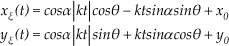
The sensor distance d_θ is measured in an opportune rotation step when the motor is stopped (stopping positions) and it is ideally the minimum distance between the sensor position (x₀,y₀) and the target line on condition that the sensor is able to catch the reflection according to the directivity diagram and the law of reflection. In Figure 2 the region (whose boundary is indicated as a dotted curve) and the minimum distance direction (shown as a marked and dotted line) are plotted for θ=60°, r=15 cm, α=85° and k=400 cm.

Figure 1.

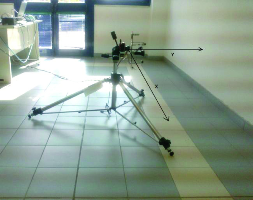
The mechatronics scanning device.

In the plot the target line is obtained for β=30° and q=110 cm. In this case the target point (also called the reflecting point) is inside the bounded region (successful detection). The distance d_θ measured by the sensor in this condition may be calculated by (5).

d_{θ} = x_{0} s i n β + (q - y_{0}) c o s β

(5)

In Figure 3, the same parameters (β=30° and q =110 cm) and configuration (r=15 cm, α=85° and k=400 cm) are considered, but the target point is outside the bounded region (unsuccessful detection) when the position is θ=0°. In this case the sensor is not able to return the time of flight and the distance value de may be equally imposed to the measure range k. When successful detection occurs, the reflecting point may be transformed in such a way as to plot the point P_r expressed by (6).

P_{r} = [\begin{matrix} (d_{θ} + r) c o s θ & (d_{θ} + r) s i n θ \end{matrix}]

(6)

On the contrary, in the case of unsuccessful detection, point P_l may be considered as laying both on the boundary and on the region axis. Its coordinates are expressed by (7).

P_{l} = [\begin{matrix} (k + r) c o s θ & (k + r) s i n θ \end{matrix}]

(7)

The model considers that the maximum sound pressure of the ultrasonic sensor is along the region axis of the cone [7] and that the wave pressure decreases very deeply outside. The semi-aperture angle α is directly connected with the horizontal directivity of the sensor, including the effects of eventual lateral lobes.

2.1. Model Validation

In order to compare the theoretical points with experimental ones, several tests were conducted by propagating ultrasonic waves towards a regular wall. The tripod was located in front of the wall at a minimum distance sensor-wall d_min = 103cm along the y-axis. The motor was programmed to take 40 steps in the angular interval [0° 180°]. Each experimental point was calculated by substituting the measured distance value d_s for dθ in (6). The same formula (7) was used when the echo was not caught (a range k=400cm was fixed in both the considered cases). The angular correspondence between the sets of points is clearly linked to the correct estimation of the beam visibility angle α. The value α=85° was established for the used sensor because it gave excellent correspondence in all the experiments. Different observer locations were considered by manually changing the sensor starting position and reading it on a goniometer placed on the tripod. The comparison plot between the experimental and the theoretical data for some of the executed tests is shown in Figure 4 (β=-30°, 0°, 30°, 60°). The validated model may well predict the experimental result and the estimated visibility angle α permits the accurate identification of successful or unsuccessful detections.

Figure 2.

The bounded region for θ=60°, α=85°, β=30°, r=15 cm and k=400 cm (successful detection).

Figure 3.

The bounded region for θ=0°, α=85°, β=30°, r=15 cm and k=400 cm (unsuccessful detection).

Figure 4.

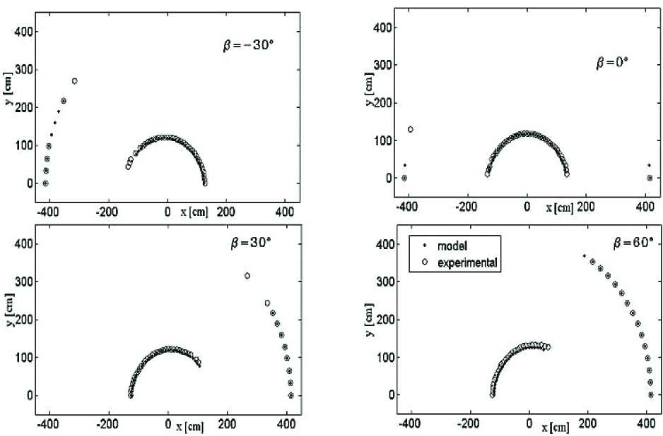
Comparison between the experimental and the theoretical data.

3. Three Different Ways for Detecting the Wall Orientation

The validated model allows the possibility of testing the approaches for detecting a regular wall and allows the evaluation of their sensitivity to the number of rotation steps. Seventeen different configurations were considered, so as to have β varying from −80° to 80° with differences of 10°. The distances concerned with successful detections are shown in Figure 5 for each motor position. In Figure 6 the theoretical distance values are compared with the distance values perturbed by means of a random additive noise. Two different levels of maximum noise were considered in order to have a perturbation of 1% and 2% respectively.

It is clear that the data corrupted by 2% of maximum random noise better simulated the experimental conditions. Therefore, they were carefully used for testing the proposed approaches at increasing the dataset cardinality. Moreover, one should consider that the theoretical dataset does not feel the effect of the inaccurate manual β yaw-rotation that occurs in the experimental setup.

3.1. Second-Order Taylor Based Approach for Minimum Distance Estimation

To achieve the aim of determining the target orientation, the first and simplest method analysed here is based on observations of the measured distances in each pointing direction. Considering the distances in Figure 5, their minimum value is close to the position defined by 90°+β. A fitting parabola is obtained by the Least Squares Method (LSM) and its equation is used for estimating the slope angle β. The slope is calculated as θ_min-90°, where θ_min is the value where the tangent line to the parabola has a slope of zero. This method permits us to discover the relative orientation of a regular corridor wall but it does not attribute any confidence to the result. The choice to fit by a parabola is due to the fact that it is close to the second order Taylor approximation of the theoretical data at 90°+β.

3.2. PCA-Based Approach Using the Covariance

The necessity of ascertaining whether the wall was regular (without any openings) or other obstacles were interposed between the sensor and the wall induced the authors to consider a new approach. This idea was based on the PCA [16], which consists of an orthogonal transformation to convert a cloud of points to a new reference where the principal coordinates (also called principal components) have the greatest variance possible. This mathematical procedure is typically used in exploratory data analysis and it may be computed by calculating the covariance matrix of the data. The points of Figure 4 may be arranged to obtain a matrix X of dimensions 2×N, where N is the number of pointing directions. The vector Y, that indicates the deviation of X components from the mean values, is calculated by (8), where the mean vector w is defined in (9) and h is the all ones N dimensional row vector.

Y = X - w \cdot h

(8)

w = [\begin{matrix} \frac{1}{N} \sum_{n = 1}^{N} X (1, n) \\ \frac{1}{N} \sum_{n = 1}^{N} X (2, n) \end{matrix}]

(9)

The covariance matrix C has dimensions of 2×2 and is defined by (10).

C = \frac{1}{N - 1} Y Y^{T}

(10)

This matrix is symmetric and its determinant is positive. It may be linked to the equation of a set of ellipses defined by (11), where c_ij {i,j=1,2} is the generic element of C and C₃₃ is a negative parameter, which has to be fixed in order to draw an ellipse of the set.

c_{11} {\tilde{x}}^{2} + c_{22} {\tilde{y}}^{2} + 2 c_{12} \tilde{x} \tilde{y} + c_{33} = 0

(11)

Indicated by λ_min and λ_max, the minimum and the maximum eigenvalue of C, it is possible to define the eccentricity of the ellipse as in (12), where EVR is the ratio λ_min/λ_max.

Figure 5.

Experimental distances measured in case of successful detection.

Figure 6.

Theoretical distances carried out by the model and perturbed distances by means of random noise.

e = \sqrt{1 - E V R}

(12)

When the corridor wall is scanned, the eigenvalues of C are very different and the resulting ellipse is quite flattened. According to [11], a range for the parameter e may be defined in order to warrant the absence of holes in the wall and to exclude the following slope estimation in case of undesired objects. These objects may be responsible for unexpected reflections [13]. The theoretical and experimental curves, obtained by the eccentricity values relating to different slopes, are plotted in Figure 7 (N=41 pointing directions are considered in the scanning straight angle). In the case where the target wall is regular, the eccentricity is greater than 0.7 (e > 0.7). When the detected target presents some discontinuities or undesired obstacles interposed between the sensor and the scanned surface, the parameter e gets lower. Therefore, a preliminary analysis of the parameter e permits the verification of both the regularity of the wall and the free path for the waves.

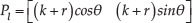
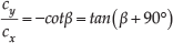
The eigenvectors associated with the eigenvalues of the matrix C are orthogonal to each other and they describe the direction of the axes of the ellipse defined by (11). If the matrix X is built considering only the data concerned with successful detections (measured distance lower than a threshold [13]), it is very interesting to observe that there is a direct relationship between β and the clockwise rotation angle γ for expressing the ellipse (11) in canonical form with the major axis corresponding to the vertical axis. The relationship between β and γ introduced in [11] considers the equality of β and γ when γ is inside the angular interval [α-90°,90°-α]. In fact, in this interval the successful reflection points define a full arc. The equality of β and γ may be proved by considering the line passing through the outermost points of this arc. In this case, the orientation β of the target wall is given by γ. Outside such an interval [α-90°,90°-α], the successful reflections do not create a full arc, but only a part of one (Figure 8). Therefore, the slope of the line connecting the outermost points does not correspond with β. Defining P₁ (x₁₂, x₂₂) and P₂ (x₁₁, 0) as the extreme points of the detected arc (Figure 9), it is possible to consider the line connecting the points P₁ and P₂ for proving that the matrix C, obtained by only these two points, has a null eigenvalue. The angle γ formed by a straight line with a vertical axis may be linked with the target orientation angle β. Formulas (13-15) express the coordinates of the points P₁ and P₂ in a generic parametric way.

x_{11} = - s \cdot k_{X} + r s i n β

(13)

\begin{array}{l} x_{12} = s \cdot k_{X}_{} s i n_{} (α + β) + \\ + \frac{1}{2} [r_{} s i n_{} β_{} (1 - c o s_{} (2 \cdot α + 2 \cdot s \cdot β)) - s \cdot r c o s_{} β_{} s i n_{} (2 \cdot α - 2 \cdot s \cdot β)] \end{array}

(14)

\begin{array}{l} x_{22} = k_{X}_{} c o s_{} (α - s \cdot β) + \\ - \frac{1}{2} [r_{} c o s_{} β_{} (1 + c o s_{} (2 \cdot α - 2 \cdot s \cdot β)) - s \cdot r s i n_{} β s i n_{} (2 \cdot α - 2 \cdot s \cdot β)] \end{array}

(15)

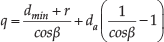
s is the sign function applied to β (s=sign(β)) and kx is defined by (16).

k_{X} = d_{a} (1 - c o s β) + d_{m i n} + 2 r

(16)

d_a is the perpendicular distance between the motor axis and the tripod axis and d_min is the minimum distance sensor-wall when β=0° and θ=90°.

Figure 7.

Eccentricity parameter.

Figure 8.

Described arc (β=-45°, α=85°).

Figure 9.

Points considered for the estimation of β when γ is outside the interval [α-90°,90°-α] (β=-45°, α=85°).

Equations (12-15) have a generic validity for any type of device geometry and for any type of sensor directivity. In the case being considered, they give the following relationship for when γ is outside the angular interval [α-90°, 90°-α].

β = 1.861 γ - s \cdot 4.306 °

(17)

Another important aspect of this approach is that the proposed analysis does not depend on the value d_min.

3.3. Approach Based on a Fitting Circumference

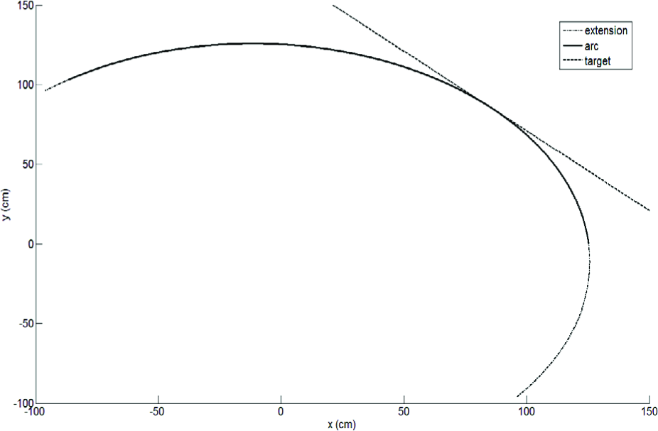
Another approach introduced and discussed here concerns with the possibility of fitting the detected points P_r by a circumference. It is possible to demonstrate that the ratio of the coordinates of the centre C (c_x, c_y) is defined by (18).

\frac{c_{y}}{c_{x}} = - c o t β = t a n (β + 90 °)

(18)

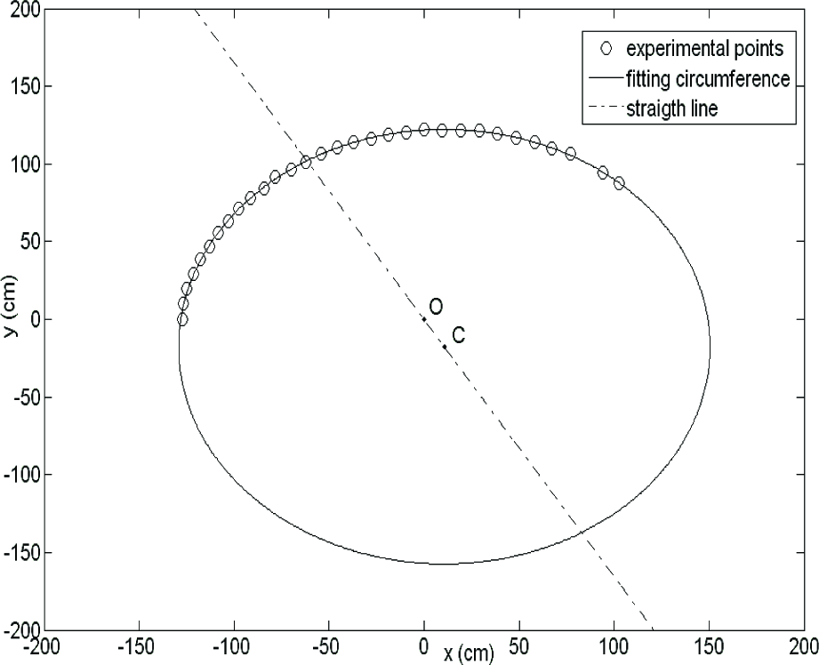
The coefficients of the equation of this circumference may be estimated through a minimization procedure. In Figure 10 the circumference is obtained for the data from Figures 8 and 9. The target slope β is defined by considering the straight line passing through the centre C and the origin O of the reference system. A non-linear least squares method has been used to find the circumference.

It converges in a few steps in all cases. In Figure 11 the application of this method to one experimental case (β=30°) is shown.

4. Experimental Tests and Comparison

The three techniques were tested on the experimental data obtained with the rotating sensor, located in front of a regular wall. The use of a professional tripod, which was equipped with a level gauge, assured correct placement and it satisfied the need for rotating the actuator. In this way, the wall appears rotated with respect to the new reference system of angle β. The scheme of the scanning device in two different configurations is indicated in Figure 12, where the line of intersection between the wall and the sensor rotation plane is also plotted.

The target is represented by the straight line, which has a y-intercept q, as expressed by (19) and a slope angle β within (-90°,90°). The automatic sensor rotation describes a circle radius of r=15cm, the actuator rotation describes a circle radius of d_a=10cm and the minimum distance sensor-wall is d_min=103cm. The estimation of β permits the calculation of q by (19).

Figure 10.

Fitting Circumference approach (β=-45° and α=85°).

Figure 11.

Fitting Circumference approach for the experimental data (β=30°).

Figure 12.

The scheme of the scanning device in two different configurations.

q = \frac{d_{m i n} + r}{c o s β} + d_{a} (\frac{1}{c o s β} - 1)

(19)

After that the configuration is changed by manually rotating the actuator around the tripod axis. The digital motor may be programmed to accomplish the desired number of rotation steps. In fact, the driving code was developed in order to let the sensor move describing a straight angle.

The three approaches were tested on the set of 17 different target configurations. The tripod was rotated so as to propose 17 different experiments with β varying in [-80°,80°] and with steps of 10°. The modular actuator was programmed to take 40 rotation steps (41 pointing directions) in each configuration and the distance measurement was carried out in each rotation step. In Table 1 the experimental results of the Least Squares Method (LSM), PCA and Fitting Circumference (FC) are shown. It is important to consider that the expected slope angle (starting tripod rotation) was manually measured by a goniometer, introducing an error to the real position. The average absolute error μ of the absolute orientation error for all tests is shown in the last row of Table 1 and is quite low for all these techniques.

Table 1.

Experimental results of the three approaches with 41 pointing directions

β[°]	LSM	PCA	FC
−80	−69.94	−81.11	−69.32
−70	−68.84	−68.97	−66.98
−60	−56.11	−56.27	−55.30
−50	−47.22	−50.77	−47.24
−40	−36.37	−28.91	−36.52
−30	−25.45	−15.52	−25.73
−20	−15.83	−11.84	−16.33
−10	−8.44	−4.31	−6.88
0	2.49	−1.00	2.63
10	12.21	15.39	12.22
20	22.38	15.06	22.75
30	30.93	35.49	31.17
40	41.37	41.76	41.49
50	50.56	43.87	50.13
60	60.79	57.08	60.03
70	74.47	66.82	71.55
80	80.85	86.36	79.89
µ	2.81	4.89	2.81

For the aim of discussing and testing the three strategies, the simulated data have also been taken into account. By applying these strategies to the data without perturbing them, it is possible to correctly estimate β in all cases. The robustness of these approaches is analysed afterwards by introducing noise, as previously discussed. Table 2 shows the results when the imposed maximum error is 2% (the same error considered for the three simulations) with the same number of pointing directions (41) used in Table 1 for the experimental data.

Table 2.

Results of the three approaches with 41 pointing directions on the simulated data with 2% of maximum noise introduced

β[°]	LSM	PCA	FC
−80	−82.42	−80.36	−81.59
−70	−68.05	−71.23	−67.96
−60	−58.27	−62.03	−58.40
−50	−49.33	−52.74	−49.80
−40	−39.04	−39.53	−39.49
−30	−29.57	−30.43	−29.96
−20	−19.84	−21.48	−20.21
−10	−10.39	−12.59	−10.51
0	−0.46	−0.07	−0.56
10	8.39	12.46	8.41
20	18.04	21.30	18.31
30	27.65	30.22	28.03
40	37.17	39.33	37.77
50	47.70	52.55	48.48
60	57.66	61.84	58.39
70	68.34	71.09	69.12
80	78.99	80.37	80.18

The methods are comparable and give good results for all the tests. The final results are quite similar to the experimental ones. For a low number of points (41), the LSM, PCA and FC approaches have similar behaviour. In order to evaluate the sensitivity with respect to the number of points in the same scanning range, other simulations were carried out by increasing the number of pointing directions from 41 to 60, 90, 120 and 180. In Tables 3 and 4 the results from 90 and 180 positions are shown.

Table 3.

Results of the three approaches with 90 pointing directions on the simulated data with 2% of maximum noise

β[°]	LSM	PCA	FC
−80	−90.99	−82.03	−88.29
−70	−74.20	−71.75	−73.30
−60	−62.61	−61.42	−62.37
−50	−51.24	−51.09	−51.49
−40	−39.85	−40.86	−40.23
−30	−29.38	−30.73	−29.78
−20	−19.31	−20.68	−19.55
−10	−9.82	−10.77	−9.83
0	0.26	0.04	0.31
10	9.84	10.95	9.96
20	19.16	20.83	19.48
30	28.64	30.85	29.10
40	38.25	40.94	38.72
50	48.27	51.13	48.75
60	58.25	61.43	58.52
70	66.22	71.71	66.30
80	78.51	81.83	78.31

Table 4.

Results of the three approaches with 180 pointing directions on the simulated data with 2% of maximum noise

β[°]	LSM	PCA	FC
−80	−79.01	−80.61	−79.49
−70	−70.38	−70.30	−70.61
−60	−58.90	−60.07	−59.28
−50	−48.07	−49.88	−48.56
−40	−38.10	−39.74	−38.64
−30	−28.20	−29.68	−28.66
−20	−18.30	−19.72	−18.63
−10	−8.57	−9.89	−8.67
0	1.15	0.01	1.17
10	10.68	9.97	10.84
20	20.27	19.85	20.66
30	30.41	29.85	30.89
40	40.57	39.96	41.05
50	50.97	50.15	51.31
60	62.11	60.38	62.22
70	74.01	70.65	73.69
80	86.72	80.91	86.11

Tables 3 and 4 show that the increase in the number of rotation steps does not result in substantial improvements for the LSM and the FC approach, which are the common strategies used in literature. On the contrary, the PCA-based method converges to the correct values by increasing the number of points. This behaviour can be emphasized (Table 5 and Figure 13) by considering the average μ of the absolute orientation error as a unique parameter on all 17 considered configurations.

Table 5.

Average absolute error μ of the three approaches on the simulated data with 2% of maximum noise

Pointing directions	LSM	PCA	FC
41	1.48	1.29	1.11
60	3.15	1.30	2.98
90	1.99	1.12	1.63
120	1.89	0.40	1.41

The results confirm the applicability of the proposed methods by means of the rotating device and the simulations predict that by increasing the number of rotations in the measurement range the experimental error may be significantly reduced when the PCA is computed. Of course, the results shown herein can help to find a reasonable compromise between the estimation accuracy and the number of motor steps required. Finally, it is interesting to specify that using the PCA-based method gains preliminary information on the absence of openings in the wall, as well as the presence of unforeseen objects. It is therefore generally more effective than the other approaches.

5. Conclusion

In this paper the authors have suggested three different techniques all based on the geometrical properties of sound reflection in order to estimate the parameters of a plane, such as the wall of a corridor. They have used a rotating device of their own design in which a sensor is able to spread a wide ultrasonic beam. The proposed approaches have been tested by a theoretical model of the ultrasonic propagation and successively such model was perturbed with a random error in order to simulate the experiments. The possibility of evaluating the outcome of changing the target configuration and the number of pointing directions allowed the authors to carry out a complete sensitivity analysis and to take the effect of undesired reflections into account. The PCA-based approach proved to be better than the other classic methods as a result of a very low medium error (less than 0.5°) obtained when increasing the dataset cardinality. The results are very satisfactory and they encourage further research with a view to planning the path for a mobile robot. Although most robotics applications make use of complex laser systems for attaining the aims of localization, the authors encourage the use of ultrasonic sensors. Ultrasonic systems are essential in case of low visibility or environments surrounded by mirrors, transparent surfaces or light-absorbing obstacles in which lasers often fail. The future aim is to equip a robot with the ultrasonic scanner in such a way as to take advantage of the parameter evaluation in path planning. The authors also plan to evaluate the possibility of fusing information from other sensors, such as infrared-based sensors.

Figure 13.

Average absolute error μ for the three approaches on the simulated data with 2% of maximum noise perturbation.

References

Crowley

(1985) Navigation for an intelligent mobile robot. IEEE Trans. on Robotic and Automation, RA-1: 31–41.

Moravec

Elfes

(1985) High resolution maps from wide angle sonar. Proc. of the IEEE Int. Conf. Robotics and Automation: 116–121.

Kuc

Siegel

(1987) Physically based simulation model for acoustic sensor navigation. IEEE Trans. on Pattern Analysis and Machine Intelligence, PAMI-9: 766–778.

Barshan

Kuc

(1990) Differentiating sonar reflections from corners and planes by employing an intelligent sensor. IEEE Trans. on Pattern Analysis and Machine Intelligence, 12: 560–569.

Choset

Nagatani

Lazar

(2003) The arc-transversal median algorithm: A geometric approach to increasing ultrasonic sensor azimuth accuracy. IEEE Trans. on Robotics and Automation, 19: 513–522.

Barshan

(2007) Directional processing of ultrasonic arc maps and its comparison with existing techniques. Int. Journal of Robotic Research, 26: 797–820.

Lee

Chung

(2009) Effective maximum likelihood grid map with conflict evaluation filter using sonar sensors. IEEE Trans. on Robotics and Automation, 25: 887–901.

Lee

Doh

Chung

(2010) An exploration strategy using sonar sensors in corridor environments. Intelligent Service Robotics, 3: 89–98.

Giannoccaro

Spedicato

di Castri

(2011) 3D reconstruction of L-shaped surfaces using a rotating array of ultrasonic sensors. Proc. of the IEEE International Multi-Conference on Systems Signals and Devices, pp. 1–7, IEEE Xplore Digital Library. DOI: 10.1109/SSD.2011.5767483.

10.

Giannoccaro

Spedicato

di Castri

(2012) A new strategy for spatial reconstruction of orthogonal planes using a rotating array of ultrasonic sensors. IEEE Sensors Journal, 12: 1307–1316, DOI: 10.1109/JSEN.2011.2170062.

11.

Giannoccaro

Spedicato

(2012) A PCA-based interpretation of ultrasonic data for accurately detecting a corridor wall. Proc. of the IEEE International Multi-Conference on Systems, Signals and Devices (Sensors, Circuits and Instrumentation Systems), IEEE Xplore Digital Library.

12.

Durrant-Whyte

Bailey

(2006) Simultaneous localization and mapping: Part I. IEEE Robotics.

13.

Durrant-Whyte

(1992) Directed Sonar Sensing for Mobile Robot Navigation. Norwell

, MA: Kluwer.

14.

Sorenson

editor (1985) Kalman Filtering: Theory and Application. IEEE Press.

15.

Lee

Cho

D-W

Song

(2012) Novel Sonar Salient Feature Structure for Extended Kalman Filter-Based Simultaneous Localization and Mapping of Mobile Robots. Advanced Robotics, 26: 1055–1074.

16.

Basilevsky

(1994) Statistical analysis and related methods, theory and applications. Wiley Online Library.

Three Different Approaches for Localization in a Corridor Environment by Means of an Ultrasonic Wide Beam

Abstract

Keywords

1. Introduction

2. A Model for the Ultrasonic Propagation

2.1. Model Validation

3. Three Different Ways for Detecting the Wall Orientation

3.1. Second-Order Taylor Based Approach for Minimum Distance Estimation

3.2. PCA-Based Approach Using the Covariance

3.3. Approach Based on a Fitting Circumference

4. Experimental Tests and Comparison

5. Conclusion

References