Sage Journals: Discover world-class research

Abstract

In this paper, the authors make use of sonar transducers to detect the corner of two orthogonal panels and they propose a strategy for accurately reconstructing the surfaces. In order to point a linear array of four sensors at the desired position, the motion of a digital motor is appropriately controlled. When the sensors are directed towards the intersection between the planes, longer times of flight are observed because of multiple reflections. All the concerned distances have to be excluded and that is why an indicator based on the output signal energy is introduced. A clustering technique allows for the partitioning of the dataset in three clusters and the indicator selects the subset containing misrepresented information. The remaining distances are corrected so as to take into consideration the directivity and they permit the plotting of two sets of points in a three-dimensional space. In order to leave out the outliers, each set is filtered by means of a confidence ellipsoid which is defined by the Principal Component Analysis (PCA). The best-fit planes are obtained based on the principal directions and the variances. Experimental tests and results are shown demonstrating the effectiveness of this new approach.

Keywords

Sonar Sensors Mechatronics Device Signal Processing Automatic Classification Statistical Data Analysis Data Fitting

1. Introduction

The aim of perceiving an environment is ambitious in mechatronics because it lets a robot operate avoiding collisions. Expensive devices, such as laser sensors or camera systems, are often preferred to ultrasonic sensors in spatial reconstructions owing to the disadvantages of sound propagation. Although the latter light-based sensors are very accurate, they are not able to work in some conditions such as smoky rooms, or in the presence of light-absorbing or shining obstacles [1]. Therefore, ultrasonic sensors, also called in-air sonar sensors, are mostly used in these particular scenarios, even if their low-cost often leads researchers more and more to test their use in common home-like environments. These sound-based sensors spread mechanical waves through the air and they wait for the echoes. The elapsed time between the transmission start and the reception is the Time Of Flight (TOF) and it is proportional to the travelled distance. Several TOF measurements are generally required to estimate the distance and different methods may be compared in a statistical way [2]. The TOF values depend on the speed of sound and, as such, digital signal processing techniques prove to be a necessity for compensating for the speed variations due to temperature or other atmospheric conditions [3]. In industry, sonars are widely employed for controlling the liquid level in containers taking advantage of the sound reflection on the surface of liquid. The authors recently designed a mechatronics device for measuring the water level in a tank and for estimating the volumetric flow [4]. A lot of research is aimed at interpreting the collected data for localizing and classifying some target obstacles [5]. Other works allow for the detection of the size and shape of the reflecting object using neural networks and considering amplitude, frequency and time structure [6]. Moreover, the echoes may be processed and from this energy, duration and range can be extracted so as to characterize the roughness and the orientation of the reflecting surface [7]. In some cases, the reflector geometry is such as to make the use of a multisensory sonar system more preferable than a single sensor. These systems may be advisable for tracking an object and identifying it [8] especially in conditions in which it is not possible to use other sensors. Since the sound wave front is spherical, more sensors have to be fired to locate a spherical target and to estimate its curvature [9]. Some further studies are concerned with the conversion of geometrical shapes into quantitative values. The goal of detecting openings in a wall is achieved by means of the PCA which makes it possible to attribute a scalar value to a set of points [10]. The authors have also tackled a similar problem and they have proposed a model for evaluating the regularity of a wall and for estimating its orientation [11]. Sonar sensors may be utilized to build a map of the surrounding environment. A recent processing approach for ultrasonic arc maps is proposed in [12] and compared to six other existing traditional techniques [12]. The difficulty of equipping robots with sonars is frequently due to the wide sound beam propagated, which is responsible for TOF measurements and is significantly affected by many factors, such as specular reflections and scattering. In previous studies, the authors used a new model of ultrasonic sensors able to produce an analogue sonic signal (full waveform) as well as a logic signal including information on the TOF. The authors implemented an array of four sensors moved by a digital modular actuator [13] and then utilized it to scan and reconstruct an L-shaped obstacle [14]. After this, they carefully examined the physical phenomenon of multiple reflections in the zone close to the intersection and they introduced a new reconstruction strategy based on the Fuzzy C-Means (FCM) algorithm and on the RANdom SAmple Consensus (RANSAC) fitting [15]. They have brought together the previous analyses and observations in such a way as to define a new procedure in which each best-fit plane is obtained by statistical considerations. Numerous tests have confirmed that the energy of the analogue sonic signal increases if the sensor is pointed at the intersection and a new indicator of the relating motor position is herein introduced. This indicator proved to be preferable in more cases particularly when some sensors are not able to catch reflection. The values of this indicator, the distances and the motor positions permitted us to define a cloud of points which was partitioned into three clusters by the FCM algorithm. One of these clusters contains spurious distances due to multiple reflections and it is selected by the maximum value of the indicator. The remaining sets have been used to plot some points in a three-dimensional space taking into account the directivity diagrams. The aim of excluding eventual outliers has been pursued by calculating the covariance matrix of each set. The eigenvectors of this matrix give the directions of the axes of an ellipsoid, whose centroid corresponds to the mean point and the eigenvalues allow for the fixing of the length of the axes so as to contain all the inliers in it. The new covariance matrix of each filtered set permits us to obtain the normal vector of each plane and the equation may be fully determined assuming that the plane passes by the new mean point. The aim of accurately reconstructing two orthogonal planes by using ultrasonic sensors is very interesting in industrial robotics applications. For instance, fabrication processes often consist in joining together two parts by using welding robots [16–17]. The automatic welding solutions are more and more desired to reduce imperfections and to improve the final quality [18]. Since the welding process is complex, the interaction human-robot is generally essential. The proposed reconstruction strategy could be applied to the specific problem of joining two flat surfaces together. In this way, a welding robot could become aware of the obstacle's location and the need for human intervention could be limited. Many experiments were carried out and the most meaningful ones are herein discussed.

2. The Sonar Sensor Array for Estimating the Distance

The rotating array is moved by means of a servo modular actuator Dynamixel AX-12+ [19]. This smart system consists of a precision motor and a control circuitry which is connected to a computer in order to drive the rotation of a frame by using the Universal Serial Bus (USB) [19]. The actuator was placed on an extendible professional tripod and its shaft was constrained to a plastic thick bar on to which four sensors were screwed. The linear array is composed of two types of ultrasonic sensors: Hagisonic AniBat HG-M40DAI and HG-M40DNI [20]. These sonar sensors are both transmitters and receivers of ultrasonic waves at a frequency of 40 kHz [20]. The HG-M40DAI sensor spreads an anisotropic beam and it may detect obstacles up to 4 m away with a horizontal directivity of about 150° and a vertical directivity of about 60°−70° [20]. The HG-M40DNI sensor spreads an isotropic beam up to 9 m and it has a directivity of 10° [20]. The capsules are placed alternately at a distance of d_s = 8 cm. The rotating device is illustrated in Figure 1, where the HG-M40DAI models are labelled with the numbers “1” and “3” while the HG-M40DNI models are labelled “2” and “4”.

Figure 1.

Mechatronics scanning device

The sensors are able to rotate around the x axis of the reference system indicated in Figure 1. Whenever an input pulse is applied to an opportune wire (several shapes are available), the ultrasonic transmission is driven at its rising edge [20]. In the proposed tests the chosen input signal is rectangular with a frequency of 12.5 Hz, a duty cycle of 4% and an amplitude of 4 V. The use of a rectangular signal is recommended by the sensor producer [20] and it could be easily obtained by means of an oscillator circuit. Moreover, preliminary calibration tests showed the sensor operates well with the chosen input signal. All the sensors are powered by a recommended voltage of 12 V and a red intermittent Light Emitting Diode (LED) indicates whether it is working correctly. When the reflected wave is detected, the sensor responds to the input pulse with a subsequent output pulse. The TOF may be estimated by the period elapsed from the rising edge of the input pulse to the rising edge of the output pulse. The sensors were simultaneously triggered so that the waves were added together and all the output signals were acquired by the acquisition board NI-USB 6210 [21]. They were suitably sampled and processed to extract the desired information. In case of direct reflection, indicated by t_iθ, the calculated time by the i^th sensor when the motor position is θ (angle measured from the y axis to the frame direction in the yz plane), the distance may be obtained by (1) where v is the estimated speed of sound (v ≈ 345 m/s) and h is a correction factor (h = 0.922) for considering the delay of system.

d_{i θ} = \frac{h v t_{i θ}}{2}

(1)

In order to obtain a reliable distance estimation, the time t_iθ may be obtained as the median value of several consecutive measured values. In any case, the variation in measurements taken under the same conditions is very small and so the measurements are very repeatable [13 –15]. This variability test may be easily verified by considering the standard deviation and observing that its value is very low. The time values are very close to the mean.

3. The Experimental Tests and the New Indicator Based on the Signal Energy and on the Distance

The experiments are performed by using the propagation of ultrasonic waves towards the obstacle represented in Figure 2.

Figure 2.

Target obstacle and professional tripod equipped with the realized scanner

The target obstacle is obtained by placing some wooden panels on a metal structure.

In this way, two orthogonal flat surfaces may be reached by the large beam propagated and the regions of two orthogonal planes may be individualized. In spite of the multiple reflections, the purpose of this work is to draw the planes from the measured distances in each motor position. One of the real planes is normal to the y-axis and the other one is normal to the z-axis. The proposed tests are related to the same geometric configuration. The real plane normal to the y-axis has a minimum distance d_y = 157 cm from the origin of the reference system. The other plane, which is normal to the z-axis, has a minimum distance d_z = 106 cm from the same point (Figure 2). The digital motor was programmed to make a step-by-step rotation in the angular interval from −10° to 110°. The frame position was directly obtained from the control circuitry as feedback information. Two different tests were carried out in the configuration considered here with a great number of motor steps: the first test consisted of 184 steps and the second test consisted of 220 steps. Ultrasound waves were spread toward the obstacle and they returned back to the source only after the goal position was attained and when the motor was stopped. This is essential to avoiding undesired effects concerned with the motion of the source, such as the Doppler shift. The necessary experimental time for the completion of the scanning process includes the time needed to bring the sensors to the goal position and the time needed to acquire the output signals (total acquisition period). It was about 157 s for the first test and about 187 s for the second test. These times were due to the great number of rotation steps considered and to the total acquisition period of 0.8 s. The choice of such an acquisition time allowed for a reliable distance estimation from the median of the values. For the sake of reducing the scanning time, the tests can also be carried out by requiring an acquisition period of 0.08 s (only one time value for sensor in each position). In this case the scanning time goes down to about 24 s for the first test and about 29 s for the second test. Therefore, the scanning time can be reduced based on the fields of application. The time t_iθ, returned by the i^th sensor for all positions in the first and second test is plotted in Figures 3 and 4 respectively. In order to take statistical advantage of all four time values obtained in position θ, if a time value differs from the median value t_θ = median(t_1θ, t_2θ, t_3θ, t_4θ) by less or more than 20%, it is replaced by such a median value.

Figure 3.

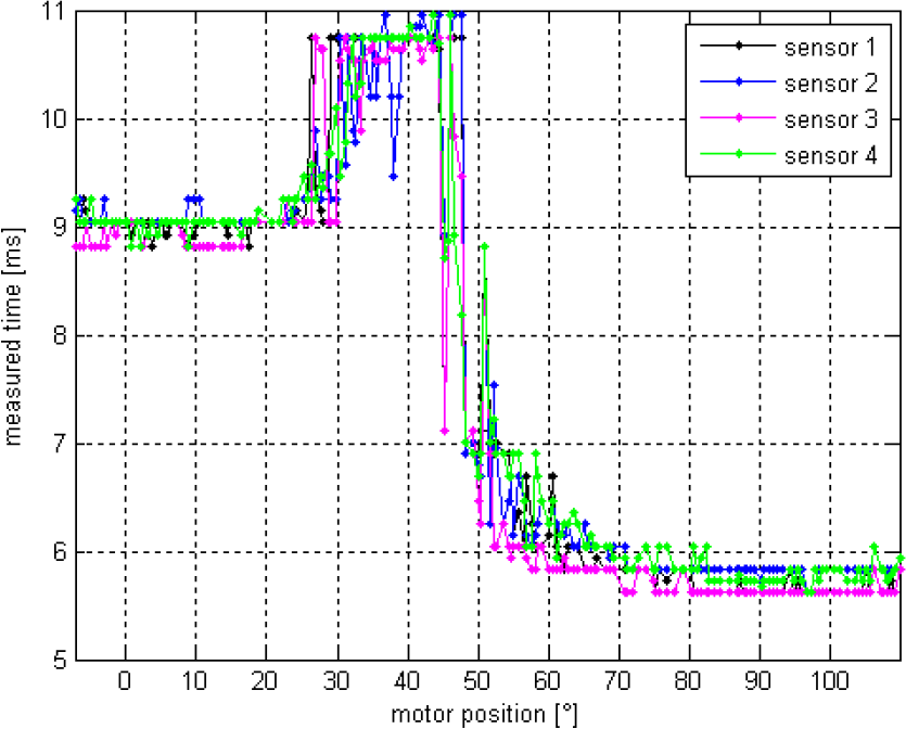
Time values measured in the first test

Figure 4.

Time values measured in the second test

As expected, many spurious time values are obtained from the zone close to the intersection. The angular position which corresponds to the intersection is θ₀ = atan(d_z/d_y) ≈ 34° (critical position). In order to exclude all the undesired values, one could choose to fix a time threshold but such an approach does not allow us to estimate θ₀ and it is not advisable in the case of an unstructured environment.

The authors intend to suggest a powerful strategy which can be generally used to reconstruct the two planes even if reflection losses or unwanted reflections occur because of irrelevant obstacles interposed between the scanner and the target. Therefore, the proposed approach could be opportunely considered in mobile robot applications. In these cases, the target may be represented by room walls on which some objects are hanging (such as pictures or lamps). In order to observe the internal crosstalk and the reflected sonic signal (analogue signal or full waveform), a wire was appropriately connected to the analogue signal test point of each sensor board [20]. The other wire extremity was plugged into the acquisition board NI-USB 6210 [21].

Let v_iθ(t) be the full waveform given by the i^th sensor in position θ, the signal energy E_iθ (expressed in V²s) may be calculated by (2), where T is the total acquisition period (T = 0.8 s in the experiments proposed).

E_{i θ} = \int_{0}^{T} v_{i θ}^{2} (t) d t

(2)

Considering the sum of the energy values for the assigned position θ, an energy level may be defined by (3), where N is the number of sensors (N = 4).

E_{θ} = \sum_{i = 1}^{N} E_{i θ}

(3)

The choice of considering the sum of the energy values is justified by the fact that the energy trend is quite similar for each sensor [18]. In Figure 5 the energy level is plotted for all the positions of the second test.

Figure 5.

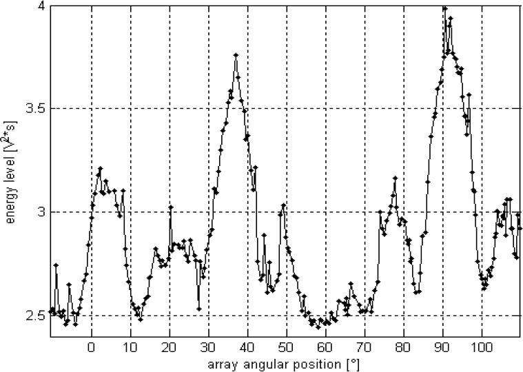
Energy level for all the positions of the second test

The energy level is high in cases of direct reflection, which happens for θ ≈ 0° and θ ≈ 90° because of the high analogue signal intensity. Moreover, the energy analysis brings out another very interesting aspect. When the beam is propagated towards the cavity due to the intersection between the panels, the signal energy increases because of constructive interference and another meaningful central peak is observed. Let us denote by d_θ the median distance, which is calculated as d_θ= hvt_θ/2, and let us consider the function W given by (4).

W (θ) = \frac{E_{θ} d_{θ}^{2}}{max_{θ} (E_{θ} d_{θ}^{2})}

(4)

This function of θ allows us to automatically select the peak concerning the critical position because it brings together both the effect of the greater energy and the effect of the greater distance measured. If θ* is the estimated value of θ₀, then θ* is such that W(θ*) = 1 (greater than any other value). One should note that the normalization of the product between the energy and the squared median distance is not necessary to detect the angular position corresponding to the plane intersection. However, this adjustment facilitates the next task of partitioning the data in order to exclude the misrepresented distances. In cases of different values for the total acquisition period (for example T = 0.08 s), a similar trend for W was verified. The indicator values are plotted in Figure 6 for the first test and in Figure 7 for the second test. In both cases, the critical position is fairly well estimated (θ* ≈ 36°).

Figure 6.

Indicator of critical position for the first test

Figure 7.

Indicator of critical position for the second test

This new indicator of the critical position proved to be better than the previous indicator introduced in [15] which was based on the dependence of the energy on the distance. In fact, when the scanning environment is not structured, reflections against non-target obstacles in the zone close to the intersection may entail an absence of the peak. In these situations, more sensors are not able to detect the target because the reflected wave amplitude is too low or the reflected wave is directed somewhere else (absence of the output pulse for estimating the TOF). The implemented code was developed in such a way as to assign the maximum detectable distance to the reflection loss. This means that, although no energy level peak is detected, the critical position can be nonetheless estimated because the indicator presents a peak due to the great distance considered. Some tests confirmed that reflection loss often takes place in a motor position close to the critical one. Therefore the use of the indicator W turns out to be very useful in these cases.

4. Reconstruction Strategy Based on Cluster Analysis and PCA

The possibility of estimating the critical angular position led the authors to use it to exclude the misrepresented distances stemming from multiple reflections. Let us consider all the points (θ_g, d_iθ, W(θ)), where θ_g is obtained by the indexed position which is the requested address value to define the motor instruction packet [15,19]. The aim of partitioning the cloud of points is pursued by means of the FCM clustering. This soft clustering allows the points to belong to three clusters and the cluster related to the critical position is left out. In this way, the original set is filtered and the spurious distance values are removed. The FCM algorithm was developed in [22] and generalized in [23]. This classification method comes from a variation of the Lloyd's algorithm which partitions the data space into a structure known as a Voronoi diagram [24]. The Fuzzy clustering is often used in machine learning, pattern recognition, image processing and bioinformatics. The proposed approach is based on the minimization of the Euclidean distances between the points and the cluster centroids through the iterative optimization of an objective function. The grade of membership of each point in each cluster is expressed by a matrix. This membership matrix was chosen as a random matrix at the first iteration and it was updated in each following iteration as long as the cost function of the improvement was less than a minimum threshold. This is equivalent to specifying a condition on the Frobenius norm of the difference between two consecutive membership matrices [15]. The fuzziness coefficient was fixed equal to 2 for updating and the minimum amount was imposed equal to 10⁻⁵. These options let us find the best location for the three sets in several experiments. The clusters of the two considered tests were mapped in the (θ, d_iθ, W(θ)) reference system and then they were plotted with different colours as depicted in Figures 8 and 9 respectively. The excluded cluster is the red one containing the point concerned with the critical position (illustrated as a black point).

Figure 8.

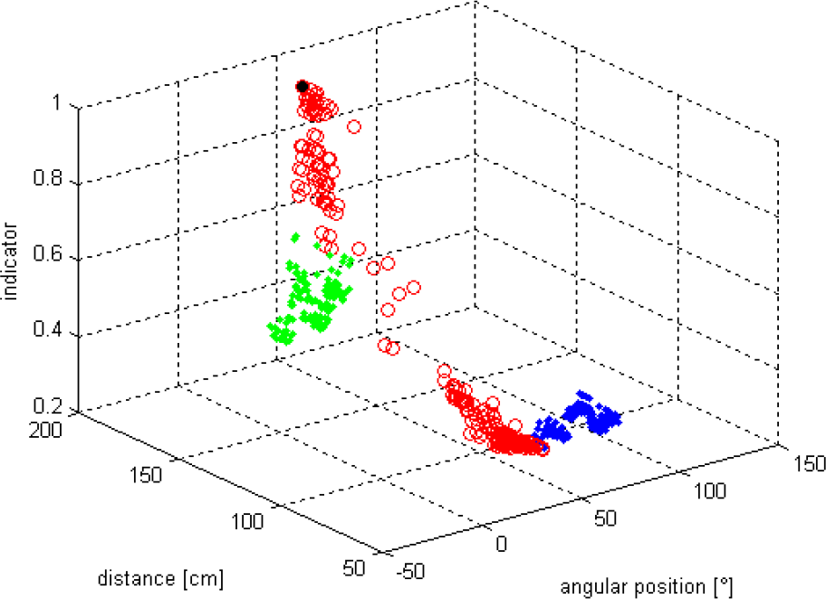
Clusters partitioned by the FCM algorithm for the first test

Figure 9.

Clusters partitioned by the FCM algorithm for the second test

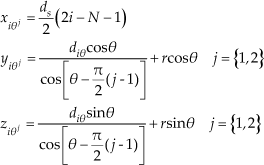
The distances d_iθ of the blue and green clusters may be used to define two sets of three-dimensional points in the reference system of Figure 1. Let (x_iθ^j, y_iθ^j, z_iθ^j) be the generic point of the j^th set such that j = 1 if θ < θ* and j = 2 if θ > θ*, the coordinates are calculated by (5) in such a way as to consider the directivity of the wide beam propagated. In the following equations, the minimum distance from each sensor capsule to the x-axis is indicated by r. Its value is about 14.5 cm for the implemented ultrasonic scanner.

\begin{array}{l} x_{i θ^{j}} = \frac{d_{s}}{2} (2 i - N - 1) \\ \begin{matrix} y_{i θ^{j}} = \frac{d_{i θ} cos θ}{cos [θ - \frac{π}{2} (j - 1)]} + r cos θ & j = {1, 2} \end{matrix} \\ \begin{matrix} z_{i θ^{j}} = \frac{d_{i θ} sin θ}{cos [θ - \frac{π}{2} (j - 1)]} + r sin θ & j = {1, 2} \end{matrix} \end{array}

(5)

The reflection scheme is indicated in Figure 10, where the effect of multiple reflections is also represented.

Figure 10.

Reflection scheme

The j^th set of the three-dimensional points allows us to arrange the data block matrix X_j which is defined by (6), where the i^th block is built as in (7) by considering all the n_i^j relating motor positions.

X_{j} = (\begin{matrix} X_{1 j} \\ ⋮ \\ X_{N j} \end{matrix})

(6)

X_{i j} = (\begin{matrix} x_{i θ_{1}^{j}} & y_{i θ_{1}^{j}} & z_{i θ_{1}^{j}} \\ x_{i θ_{2}^{j}} & y_{i θ_{2}^{j}} & z_{i θ_{2}^{j}} \\ ⋮ & ⋮ & ⋮ \\ x_{i θ_{n_{i}}^{j}} & y_{i θ_{n_{i}}^{j}} & z_{i θ_{n_{i}}^{j}} \end{matrix})

(7)

Please note that all elements on the first column of X_ij are equal. The covariance matrix C_j of X_j is given by (8), where m_j is the number of rows of X_j calculated by (9), w _j is the empirical mean vector expressed in (10) and v_j is a row vector of all those with m_j elements.

C_{j} = \frac{1}{m_{j} - 1} (X_{j}^{T} - w_{j} v_{j}) {(X_{j}^{T} - w_{j} v_{j})}^{T}

(8)

m_{j} = \sum_{i = 1}^{N} n_{i}^{j}

(9)

w_{j} = \frac{1}{m_{j}} [\begin{matrix} \sum_{i = 1}^{N} (\sum_{k = 1}^{n_{i}} x_{i θ_{k}^{j}}) \\ \sum_{i = 1}^{N} (\sum_{k = 1}^{n_{i}} y_{i θ_{k}^{j}}) \\ \sum_{i = 1}^{N} (\sum_{k = 1}^{n_{i}} z_{i θ_{k}^{j}}) \end{matrix}]

(10)

The covariance matrix C_j permits us to compute the PCA with a view to excluding the eventual outliers from each set and to getting useful information on the orientation of the planes. The PCA consists in an orthogonal transformation in order to analyse the data [10,11]. This method is frequently used in computer vision for image compression. Let λ_x^j be the eigenvalue of C_j associated with the unit eigenvector u _x ^j = (u_x1^j, u_x2^j, u_x3^j) of C_j whose rounded components are (1,0,0), let λ_y^j be the eigenvalue of C_j associated with the unit eigenvector u_y^j = (u_y1^j, u_y2^j, u_y3^j) of C_j whose rounded components are (0,1,0) and, finally, let λ_z^j be the eigenvalue of C_j associated with the unit eigenvector u_z^j = (u_z1^j, u_z2^j, u_z3^j) of C_j whose rounded components are (0,0,1). Moreover, let (x₀^j, y₀^j, z₀^j) be the mean point of the j^th set. The exclusion of the data points which are further away from the mean helps us pursue the aim of a robust estimation. The inliers are defined as all points contained in the ellipsoid which have the parametric equations given by (11), where the matrix R_j is defined in (12), the parameter ψ varies from 0 to 2π and the parameter φ varies from 0 to π. The length of the ellipsoid axes depends on the reliability factors k_x and k which were chosen in such a way as to benefit from all the sensory information (k_x = 3) and to reduce the confidence along the directions of u_y^j and u_z^j (k = 1).

(\begin{matrix} x^{j} \\ y^{j} \\ z^{j} \end{matrix}) = R_{j} (\begin{matrix} cos ψ sin φ \\ sin ψ sin φ \\ cos φ \end{matrix}) + (\begin{matrix} x_{0}^{j} \\ y_{0}^{j} \\ z_{0}^{j} \end{matrix})

(11)

R_{j} = (\begin{matrix} k_{x} \sqrt{λ_{x}^{j}} u_{x 1}^{j} & k \sqrt{λ_{y}^{j}} u_{y 1}^{j} & k \sqrt{λ_{z}^{j}} u_{z 1}^{j} \\ k_{x} \sqrt{λ_{x}^{j}} u_{x 2}^{j} & k \sqrt{λ_{y}^{j}} u_{y 2}^{j} & k \sqrt{λ_{z}^{j}} u_{z 2}^{j} \\ k_{x} \sqrt{λ_{x}^{j}} u_{x 3}^{j} & k \sqrt{λ_{y}^{j}} u_{y 3}^{j} & k \sqrt{λ_{z}^{j}} u_{z 3}^{j} \end{matrix})

(12)

The data points and the two confidence ellipsoids, which were obtained for both the tests, are represented in Figures 11 and 12. The points which are inside the closed surfaces are plotted in Figures 13 and 14.

Figure 11.

Sets of three-dimensional points and ellipsoids for the first test

Figure 12.

Sets of three-dimensional points and ellipsoids for the second test

Figure 13.

Points contained in the ellipsoids (first test)

Figure 14.

Points contained in the ellipsoids (second test)

Each excluded point of the j^th set permits the removal of the corresponding row from the matrix X_j so as to obtain a new matrix X_j*. This reduced data matrix allows us to calculate a new covariance matrix C_j* in the same way as described above. The aim of drawing the planes was soon reached. In fact, the smallest eigenvalue of C_j* is associated with a characteristic vector whose direction is normal to the fitting plane. Let us suppose that the selected unit eigenvector is n _j = (n_x^j, n_y^j, n_z^j), the equation of the plane may be expressed by (13), where the coefficient q^j is calculated as in (14) assuming that the plane passes through the median point (m_x^j, m_y^j, m_z^j) of the considered set.

n_{x}^{j} x + n_{y}^{j} y + n_{z}^{j} z - q^{j} = 0

(13)

q^{j} = n_{x}^{j} m_{x}^{j} + n_{y}^{j} m_{y}^{j} + n_{z}^{j} m_{z}^{j}

(14)

The use of the PCA allows us to achieve the very accurate reconstructions illustrated in Figure 15 for the first test and in Figure 16 for the second test. The fit planes, depicted as coloured full surfaces, are compared with the expected ones, depicted by mesh.

Figure 15.

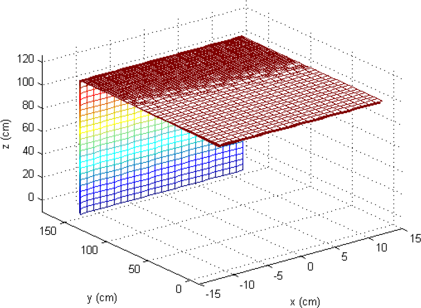
Planes reconstructed by the PCA and comparison with the real locations for the first test

Figure 16.

Planes reconstructed by the PCA and comparison with the real locations for the second test

To appreciate the validity of the proposed approach in comparison to the strategy recently introduced in [15], the equations of the fit planes were compared with the outcome of a RANSAC function [25] applied to the original sets of points calculated by (5). The RANSAC consists of a least squares estimator which similarly uses a restricted range of points (inliers). The resulting planes are plotted in Figure 17 and in Figure 18 for the two tests. As well as the previous reconstructions, the outcoming planes are compared with the real locations.

Figure 17.

Planes reconstructed by the RANSAC and comparison with the real locations for the first test

Figure 18.

Planes reconstructed by the RANSAC and comparison with the real locations for the second test

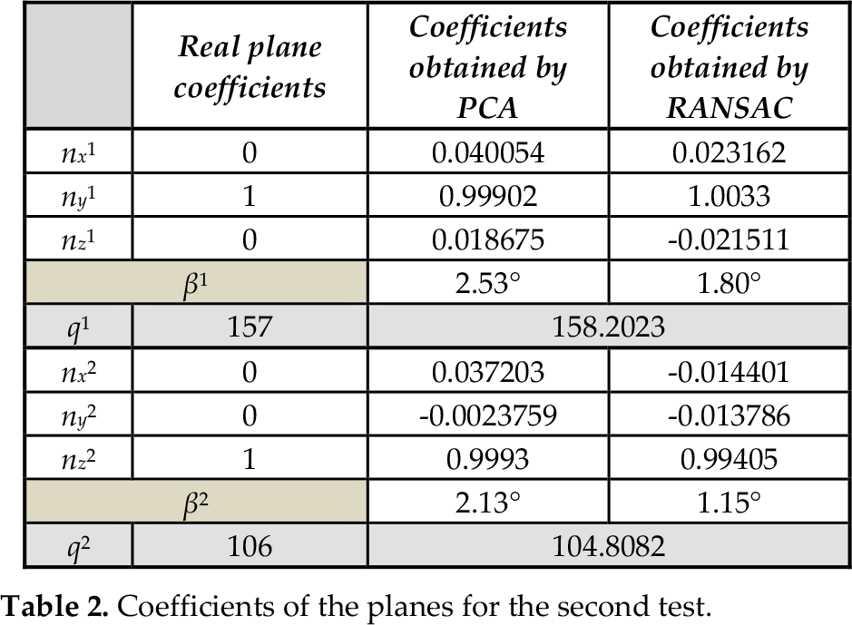
The comparison between the estimated parameters is expressed in Table 1 for the first test and in Table 2 for the second test. In both experiments they are very close to the real ones. In order to obtain the inclination of the reconstructed plane with respect to the three axes, the angle between the normal vector to the estimated plane and the normal vector to the real plane was also calculated. The angle β^j for each reconstruction is also indicated in the tables to demonstrate the effectiveness of the reconstruction strategy.

Table 1.

Coefficients of the planes for the first test

	Real plane coefficients	Coefficients obtained by PCA	Coefficients obtained by RANSAC
n_x ¹	0	0.01027	0.0070939
n_y ¹	1	0.99993	1.0043
n_z ¹	0	0.0056093	−0.045293
β ¹		0.67°	2.61°
q ¹	157	157.8116
n_x ²	0	−0.011182	−0.041207
n_y ²	0	−0.017075	−0.020819
n_z ²	1	0.99979	0.98403
β ²		1.17°	2.69°
q ²	106	103.8476

Table 2.

Coefficients of the planes for the second test

	Real plane coefficients	Coefficients obtained by PCA	Coefficients obtained by RANSAC
n_x ¹	0	0.040054	0.023162
n_y ¹	1	0.99902	1.0033
n_z ¹	0	0.018675	−0.021511
β ¹		2.53°	1.80°
q ¹	157	158.2023
n_x ²	0	0.037203	−0.014401
n_y ²	0	−0.0023759	−0.013786
n_z ²	1	0.9993	0.99405
β ²		2.13°	1.15°
q ²	106	104.8082

Both RANSAC and PCA may be used to produce results which match the set of observations very well. The more motor steps were executed in an experiment, the better the final RANSAC-based reconstructions came out because of the greater number of inliers. This improvement is not so striking because of the great number of motor steps considered in the two tests. The angle β^j is close to 0° in all the cases but the PCA-based approach is also able to operate better than RANSAC on smaller sets of point (such as the first test). On the other hand, the PCA for model fitting requires a little bit more computation effort due to the calculation of the parametric equations for the ellipsoids. The total execution time for the proposed approach was about 0.23 s for the first test and 0.29 s for the second test. The code was executed on a computer with 3.40 GHz CPU and 8 GB RAM. Hence, the clustering and PCA-based reconstruction strategy is preferable above all because the motor programming of many rotation steps causes a longer scanning process. The full FCM and PCA-based reconstruction strategy is explained by the following flow chart in Figure 19.

Figure 19.

Flow chart describing the reconstruction strategy

5. Conclusion

Nowadays, technology more and more deals with the design of robots that can help humans in several fields, such as manufacturing. A lot of research focuses on investigating new ways to let a robot become aware of its environment. Recent studies aim to endow the new generation systems with sensory abilities in such a way as to assure safety in operating. In this work the authors use an ultrasonic scanner of their own design in order to spread sound waves towards a target obstacle with the purpose of reconstructing it. When a sound beam is propagated for obstacle detection, the main difficulty stems from some undesired physical phenomena which may take place. Specular reflections may be responsible for incorrect detection. The careful examination of the related effects allows the development of a reconstruction strategy in case of multiple reflections. Since the scanning of L-shaped obstacles brings out further drawbacks to the diffuse propagation, such as undesired reflections, reflection losses and scattering, the authors take advantage of a soft clustering technique and of a statistical analysis to exclude all the spurious information and fit the planes. The proposed approach allows us to attribute a confidence to the data and each plane is drawn by the principal coordinate analysis. The objective of reconstructing the planes could be similarly attained by using laser scanners but this could be unsuitable in some scenarios. For instance, a robot could be equipped with the implemented scanner in such a way as to weld together two planes. In this case, a common laser device could fail because of the smoke. On the contrary, the sonars do not feel the effect of low visibility and they may also work in environments surrounded by high reflecting objects. The final reconstructions are very good and they provide encouragement for future studies.

References

Yang

Wang

(2008) Dealing with laser scanner failure: mirrors and windows. Proc. of the IEEE Int. Conference on Robotics and automation, pp. 3009–3015.

Barshan

Ayrulu

(1998) Performance comparison of four time of flight estimation methods for sonar signals. Electronics Letters, 34: 1616–1617, DOI: 10.1049/el:19981127.

Sabatini

(1995) A digital signal processing technique for compensating ultrasonic sensors. IEEE Trans. on Instrumentation and Measurement, 44: 869–874.

Giannoccaro

Spedicato

(2012) Ultrasonic sensors for measurements of liquid level, volume and volumetric flow in a tank. Precision Instrument and Mechanology, 1: 1–6. Available: http://www.pimjournal.org. Published by the World Academic Publishing.

Akbarally

Kleeman

(1995) A sonar sensor for accurate 3D target localization and classification. Proc. of the IEEE Int. Conference on Robotics and Automation, pp. 3003–3008.

Dror

Zagaeski

Moss

(1995) Three-dimensional target recognition via sonar: a neural network model. Neural Networks, 8: 149–160.

Bozma

Kuc

(1992) Characterizing the environment using echo energy, duration and range: the Endura method. Proc. of the IEEE Int. Conference on Intelligent Robots and Systems, pp. 813–820.

Sabatini

Rocchi

(1996) Correlation-based in air sonar sensors array for 3D object tracking and identification. Proc. of the IEEE Instrumentation and Measurement Technology Conference, pp. 371–376.

Barshan

(1999) Location and curvature estimation of spherical targets using multiple sonar time-of-flight measurements. IEEE Trans. on Instrumentation and Measurement, 48: 1212–1223.

10.

Lee

Doh

Chung

(2010) An exploration strategy using sonar sensors in corridor environments. Intelligent Service Robotics, 3: 89–98.

11.

Giannoccaro

Spedicato

(2012) A PCA-based interpretation of ultrasonic data for accurately detecting a corridor wall. Proc. of the IEEE International Multi-Conference on Systems, Signals and Devices (Sensors, Circuits and Instrumentation Systems). Available: http://www.ssd-conf.org.

12.

Barshan

(2007) Directional processing of ultrasonic arc maps and its comparison with existing techniques. The International Journal of Robotics Research, pp. 796–820.

13.

Giannoccaro

Messina

Reina

Spedicato

(2009) Ultrasonic sensors: improvements and development of an array moved by a digital servo motor. Proc. of the International Conference on Robotics, Informatics, Intelligence Control System Technologies, pp.183–189.

14.

Giannoccaro

Spedicato

di Castri

(2011) 3D reconstruction of L-shaped surfaces using a rotating array of ultrasonic sensors. Proc. of the IEEE International Multi-Conference on Systems Signals and Devices, pp. 1–7, IEEE Xplore Digital Library.

15.

Giannoccaro

Spedicato

di Castri

(2012) A new strategy for spatial reconstruction of orthogonal planes using a rotating array of ultrasonic sensors. IEEE Sensors Journal, 12: 1307–1316, DOI: 10.1109/JSEN.2011.2170062.

16.

Norberto

Pires J

Lourerio

Altino

Godinho

Ferreira

Fernando

Morgado

(2003) Welding robots. IEEE Robotics and Automation Magazine, 10: 45–55.

17.

Gerber

Gfeller

(2000) Joint connection with welded thermoplastic dowels and Wood Welding Technologies. Proc. of the World Conference on Timber Engineering.

18.

Hillbrand

Frank

(2012) Enabling automated programming of welding robots by intelligent identification of weld joints from engineering models. Proc. of the IEEE International Conference on Intelligent Engineering Systems, pp. 31–36.

19.

User's manual Dynamixel AX-12+. Available: http://www.robotis.com.

20.

Datasheet Hagisonic Ultrasonic Sensors and Timing Chart. Available: http://www.hagisonic.com.

21.

Data acquisition (DAQ) product information. Available: http://ni.com.

22.

Dunn

(1974) A fuzzy relative of the ISODATA process and its use in detecting compact well-separated clusters. Journal of Cybernetics, 3: 32–57.

23.

Hathaway

Bezdek

(1988) Recent convergence results for the Fuzzy C-Means clustering algorithms. Journal of Classification, 5: 237–247.

24.

Lloyd

(1982) Least squares quantization in PCM. IEEE Transaction on Information Theory, DOI: 10.1109/TIT.1982.1056489.

25.

Zuliani

Kenney

Manjunath

(2005) The multiRANSAC algorithm and its application to detect planar homographies. Proc. of the IEEE International Conference on Image Processing, pp. 153–156.

Clustering and PCA for Reconstructing Two Perpendicular Planes Using Ultrasonic Sensors

Abstract

Keywords

1. Introduction

2. The Sonar Sensor Array for Estimating the Distance

3. The Experimental Tests and the New Indicator Based on the Signal Energy and on the Distance

4. Reconstruction Strategy Based on Cluster Analysis and PCA

5. Conclusion

References