Inverse Kinematics of a New Quadruped Robot Control Method

Abstract

Design of redudant joints has been widely used in quadruped robots, so new kinds of techniques for sloving inverse kinematics are needed. In this paper we propose a new control method called Time-Pose control method and choose the enhanced extended jacobian matrix method for inverse kinematics. We deduce extended jacobian matrix method again so that it can be applicable for arbitrary joint length. It is argued that because the method can generate close joint angle path. With Time-Pose control method, such kind of inverse kinematics method has been used for trot gait on the flat ground. Simulations and experiments are performed, which prove the extended jacobian matrix method to be realizable for the quadruped robot.

1. Introduction

Although wheeled vehicles are very efficient, they are limited in rough terrain. Human and animals, in contrast, are capable of accessing almost anywhere. The benefit has greatly promoted the development of legged robot, such as quadruped and biped robots. Examples of such legged robots are: the biped series of Honda's ASIMO^[1] and HRP^[2]; and the quadruped series of BigDog^[3], LittleDog^[4] and HYQ^[5]. However, despite a large number of advances in the field, legged robots are still far behind their biological cousins. The key point of legged robot is the control system. In biped robot, Cardenas-Maciel^[6][7] and Oscar Castillo^[[8] have designed a kind of neural controller for generation of the walking motion.

BigDog's control system coordinates the kinematics and ground reaction forces of the robot while responding to basic postural commands. Besides central pattern generator (CPG) has been widely used for quadruped walk. Kimura^[9] generate walking patterns with a mathematical modeling of central pattern generator.

In this paper we concentrate our efforts on inverse kinematics of the quadruped control system. Quadruped robot, shown in Figure 1, has redundant freedoms in the frontal of single leg. All of its 16 active joints (four per leg) are actuated by hydraulic cylinders. As we know, the development of redundant freedoms requires the use of new techniques for solving the inverse kinematics problem. Significant examples of such techniques are: Gradient Projection method^[10] (GP), Weighted Least-Norm method^[11] (WLN) and Extended jacobian matrix^[12] (EJ) method. However, GP method does not generate closed joint space trajectories corresponding to closed end-effector trajectories, WLN method is too complex to calculate.

Figure 1.

Quadruped robot

We have presented a new control method, as shown in Figure 2, which enables quadruped robot to trot at the speed of 3km/h, carry up to 50 kg payload on the flat ground. We use the extended jacobian matrix method (EJ) instead of gradient projection method for inverse kinematics. This work extends our previous research by considering the problem of how to lift closed end-effector paths to closed joint angle paths.

Figure 2.

Control diagram of Time-Pose method

The rest of this paper is organized as follows. First, the control diagram will be proposed in Section 2. In this section, the definition of Time-Pose method will be introduced. Furthermore, the inverse kinematics methods will be introduced in Section 3. A general inverse kinematics method for different joint lengths will be deduced again in this section. Simulation and experiment results will follow in Section 4. Then the conclusion and the future works will be stated in the last Section.

2. Quadruped control

Time-Pose control method consists of gait control and pose control. In gait control, the main objective is controlling forward speed of the quadruped robot, the outputs are the location of the supporting legs and the trajectory of mass center for the next gait cycle, while the main objectives of the pose control is solving the inverse kinematics, the main outputs are joint angle (by the inverse kinematics method) or torque (by the computed torque method). Finally by means of velocity feedback the two control layers are combined together to form a closed-loop control. In this paper we only calculate joint angles in pose control, as indicated by the dotted line in Figure 2.

BigDog has successfully demonstrated that trot gait can be used for dynamic walking. Also trot gait works at low velocity, as introduced by Collins and Stewart^[13]. BigDog's trot speed reaches 1.6m/s, and the range of horse trot speed is 1.0-5.0m/s. Thus, trot gait seems to be a suitable gait for dynamic legged robots.

Gait types are defined with their order of stance phase. In this paper trot gait is chosen as the dynamic gait. At the trot gait, diagonal legs are in harmony with each other, as shown in the timing diagram of Figure. 3.

Figure 3.

Timing diagram of trot gait

In order to make the legs work together in pairs, finite state sequence has been used for trot gait. The state, shown in Figure 4, is entered when the event occurs. During trot gait states advance sequentially, A refers to the virtual leg^[14] that uses physical legs 1 and 3 (Left Front and Right Rear), B refers to the virtual leg that uses physical legs 2 and 4 (Left Rear and Right Front).

Figure 4.

State sequence of trot gait

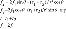
Since it is difficult to study the precise model of quadruped robot, we find some reasonable constraints which make the complex model equal to a simple model in gait control layer. The simplified model can reduce the degrees of freedom and the complexity of control. How to achieve the simplification of trotting gait model? Trot gait that caused the four legs to operate in two pairs can be viewed like an equivalent biped gait, because the members of a pair strike the ground in unison and they leave the ground in unison. In order to make the legs work together in pairs, the virtual leg method coordinates positioning of the physical legs, synchronizes ground contact, and equalizes the axial leg force. The geometry of the body also simplifies the task of positioning the physical legs, especially for trotting. The deduction is described in Equation 1. In the process, the mass of leg is ignored when compared to the torso.

$\begin{array}{l}{f}_x=f_1\sin \theta +f_2\sin \theta -{\tau }_1∕r\text{*}\cos \theta -{\tau }_2∕r*\cos \theta \\ f_y=f_1\cos \theta +f_2\cos \theta +{\tau }_1∕r\text{*}\sin \theta +{\tau }_2∕r*\sin \theta -mg\\ \tau =f_{1}d\cos \theta -f_{2}d\cos \theta +{\tau }_1+{\tau }_2\end{array}$

(1)

f,Τ,d stand for ground reaction force, hip torque and half of torso length, respectively.

If constraint exists:

$f_1=f_2$

(2)

Virtual leg can be simplified as follow:

$\begin{array}{l}{f}_x=2f_1\sin \theta -({\tau }_1+{\tau }_2)∕r\text{*}\cos \theta \\ f_y=2f_1\cos \theta +({\tau }_1+{\tau }_2)∕r\text{*}\sin \theta -mg\\ \tau ={\tau }_1+{\tau }_2\\ f=2f_1\end{array}$

(3)

Impose further constraints on virtual leg:

$\begin{array}{l}{\tau }_1\text{+}{\tau }_2=0,\\ z=z_0\end{array}$

(4)

Equation 3 equals to:

$\begin{array}{l}m\stackrel{..}{x}=f\sin \theta \\ m\stackrel{..}{z}=f\cos \theta -mg\end{array}$

(5)

The movement law of virtual leg can be simplified:

$\stackrel{..}{x}=gx∕z$

(6)

When given an initial condition, the quadruped robot will begin to move. How to control the walking speed? The answer is step length, the quadruped will be controlled in a desired speed by selecting different step length. The definition of step length is given in Figure 5.

Figure 5.

The simplification of supporting legs

$X_{step}=-\stackrel{.}{X}*T_{\mathrm{s}}∕2-K_v(\stackrel{.}{X}-{\stackrel{.}{X}}_d)$

(7)

In Figure 6 we controll the quadruped robot speed by selecting different step lengths. After adjust the step length, the robot need several cycle for symmetry. Such kind of acceleration and deceleration is the same as human running. Afterwards we need tranfer the results of Figure 6 to joint angle by inverse kinematics.

Figure 6.

Acceleration and deceleration planning

3. Inverse kinematics

When a leg is redundant, it is certain that the inverse kinematics problem admits infinite solutions. This implies that, for a given location of the leg's end-effector, it is possible to induce self-motion of the structure without changing the location of the end-effector. Leg configuration is the key point in calculating the jacobian matrix. In Figure 7 we set the connection point of the hip and leg as the base coordinate system. Relative joint angles are selected between the two rods. In this section we apply GP, WLN and EJ for squats. The results show that EJ method and WLN method can generate closed joint space trajectories corresponding to closed end-effector trajectories.

Figure 7.

The configuration of a single leg

From the configuration we have

$\left[\begin{array}{c}x\\ z\end{array}\right]=\left[\begin{array}{c}{r}_1\cos {\theta }_1+r_2\cos ({\theta }_1+{\theta }_2)+r_3\cos ({\theta }_1+{\theta }_2+{\theta }_3)\\ r_1\sin {\theta }_1+r_2\sin ({\theta }_1+{\theta }_2)+r_3\sin ({\theta }_1+{\theta }_2+{\theta }_3)\end{array}\right]$

(8)

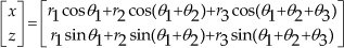
So jacobian matrix can be calculated as

$J=\left[\begin{array}{ccc}{J}_{11}& J_{12}& J_{13}\\ J_{21}& J_{22}& J_{23}\end{array}\right]$

(9)

$\begin{array}{l}{J}_{11}=-r_1\sin {\theta }_1-r_2\sin ({\theta }_1+{\theta }_2)-r_3\sin ({\theta }_1+{\theta }_2+{\theta }_3)\\ J_{12}=-r_2\sin ({\theta }_1+{\theta }_2)-r_3\sin ({\theta }_1+{\theta }_2+{\theta }_3)\\ J_{13}=-r_3\sin ({\theta }_1+{\theta }_2+{\theta }_3)\\ J_{21}=r_1\cos {\theta }_1+r_2\cos ({\theta }_1+{\theta }_2)+r_3\cos ({\theta }_1+{\theta }_2+{\theta }_3)\\ J_{22}=r_2\cos ({\theta }_1+{\theta }_2)+r_3\cos ({\theta }_1+{\theta }_2+{\theta }_3)\\ J_{23}=r_3\cos ({\theta }_1+{\theta }_2+{\theta }_3)\end{array}$

(10)

3.1 Gradient projection method

The kinematics equation describing the relationship between the end-effector velocity and joint velocities is given as:

$\stackrel{\cdot }{x}=J\stackrel{\cdot }{\theta }$

(11)

J is an mxn vector, x is an mx1 vector, and θ is an nx1 vector. For a redundant manipulator, we have m<n; therefore, an infinite number of joint velocity vectors exist for the end-effector velocity. The joint velocity vectors can be computed as:

$\begin{array}{l}\stackrel{.}{\theta }=J^{+}\stackrel{.}{x}+k(I-J^{+}J)*g\\ J^{+}=J^T{\left(J{J}^T\right)}^{-1}\end{array}$

(12)

J⁺ is the pseudo inverse of the jacobian matrix. The first item in Equation 12 is a minimum norm solution; the second item is a homogeneous linear equation solution. The first is located in the row space of the jacobian matrix, while the second is located in the null space of the jacobian matrix. Therefore, the two items are orthogonal. Since g can be any self-motion speed, optimization is accomplished by setting the proper value of g.

In squats the height of mass centre changes as a sine wave and the cycle of sine wave is 0.5s. The three methods are tested in Figure 9, Figure 10 and Figure 11, respectively. Though the height changes in the same range, the angles of joints differ from each other.

Figure 8.

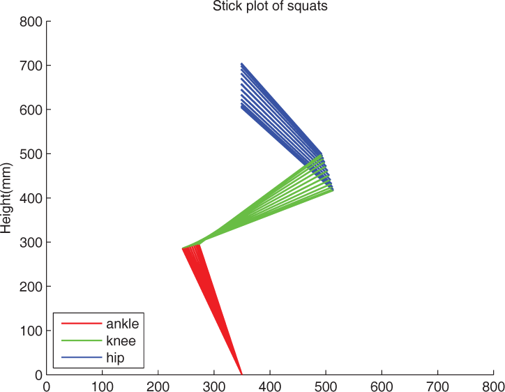
Stick plot of squats

Figure 9.

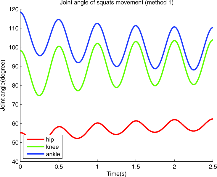
Joint angle of gradient projection method

Figure 10.

Joint angle of weighted least norm method

Figure 11.

Joint angle of extended jacobian matrix method

3.2 Weighted least-norm method

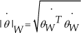
WLN has been widely utilized for minimizing energy and minimizing joint torques. In this section we utilize the WLN solution for minimizing joint velocity. We define the weighted norm of the joint velocity vector as follows:

$\begin{array}{l}|\stackrel{\cdot }{\theta }{|}_W=\sqrt{\stackrel{\cdot }{{\theta }^T}W\stackrel{\cdot }{\theta }}\\ W\in R^{n\times n}\end{array}$

(13)

W is a symmetric and positive definite weighting matrix. In most cases it will be taken as a diagonal matrix for simplicity. We introduce the following transformations:

$\begin{array}{l}{J}_W=J{W}^{-1∕2}\\ {\stackrel{\cdot }{\theta }}_W=W^{-1∕2}\stackrel{\cdot }{\theta }\end{array}$

(14)

Using Equation 11, we can rewrite Equation 14 as

$\stackrel{\cdot }{x}=J_W{\stackrel{\cdot }{\theta }}_W$

(15)

and Equation 13 as

$|\stackrel{\cdot }{\theta }{|}_W=\sqrt{\stackrel{\cdot }{{\theta }_W{}^T}\stackrel{\cdot }{{\theta }_W}}$

(16)

The LN solution of Equation 15 is:

$\stackrel{\cdot }{{\theta }_W^{\ast }}=J_W^{+}\stackrel{\cdot }{x}$

(17)

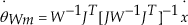
From the second part of Equation 14, the weighted least-norm solution of Equation 13 can be obtained by:

${\stackrel{\cdot }{\theta }}_{Wm}=W^{-1∕2}\stackrel{\cdot }{{\theta }_W^{\ast }}$

(18)

From the definition of pseudo inverse of jacobian matrix, the WLN solution can be written:

${\stackrel{\cdot }{\theta }}_{Wm}=W^{-1}{J}^T{[J{W}^{-1}{J}^T]}^{-1}\stackrel{\cdot }{x}$

(19)

If W is an unit matrix, then Equation 19 is the same as the first item of Equation 12. The difference between the two method is that WLN method make use of weighting matrix instead of self-motion in Equation 12. Though WLN method is lack of self-motion item, the capablily of optimization still exists. Without self-motion the method also can generate closed joint path, but computional complexity of make it worse than EJ method. Since we need real-time control, we prefer EJ method. Figure 10 shows that WLN method generate closed joint path in squats. The optimization minimize the hip joint velocity and ankle joint velocity, while in Figure 11 we know that EJ method minimaize the knee joint velocity and ankle joint velocity.

3.2 Extended Jacobian method

In this section a new method called the extended jacobian method is introduced. It is argued that because this method can lift closed end effector paths to closed joint angle paths. It provides a promising approach for the control of redundant joints of quadruped robot. Baillieul simplified the deduction by set 1 = 2 = r 3 = 1, while we have deduce the method again so that it can be used for different length of joints.

$\begin{array}{l}G(\theta )=\partial g∕\partial \theta *N_J\\ g={\left({\theta }_2-{\theta }_3\right)}^2\end{array}$

(20)

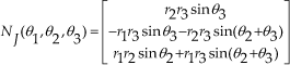
J is the jacobian matrix. If J is of full rank, there is a one dimension null space N_J. The function gis used for minimizing the knee joint velocity and ankle joint velocity.

$N_J({\theta }_1,{\theta }_2,{\theta }_3)=\left[\begin{array}{c}{r}_2{r}_3\sin {\theta }_3\\ -r_1{r}_3\sin {\theta }_3-r_2{r}_3\sin ({\theta }_2+{\theta }_3)\\ r_1{r}_2\sin {\theta }_2+r_1{r}_3\sin ({\theta }_2+{\theta }_3)\end{array}\right]$

(21)

If robot is positioned with its end effector at X so that G is extremized. Then the equation:

$\left[\begin{array}{c}F(\theta )\\ G(\theta )\end{array}\right]=\left[\begin{array}{c}X\\ 0\end{array}\right]$

(22)

Differentiating both sides, then we have the relationship between the joint angle velocity and end effector velocity:

$\left[\begin{array}{c}\frac{\mathrm{\partial }F}{\mathrm{\partial }\theta }\\ \cdots \\ \frac{\mathrm{\partial }G}{\mathrm{\partial }\theta }\end{array}\right]\bullet \stackrel{.}{\theta }=\left[\begin{array}{c}\stackrel{.}{X}\\ \cdots \\ 0\end{array}\right]$

(23)

Left item of Equation 23 can be rewritten as

$J_e=\left[\begin{array}{cc}\partial F∕\partial \theta & \partial G∕\partial \theta \end{array}\right]$

(24)

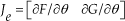
J_e is a square matrix, also we call this the extended jacobian matrix. So joint velocity can be calculated by

$\stackrel{\cdot }{\theta }=J_e^{-1}\left[\begin{array}{c}\stackrel{\cdot }{X}\\ 0\end{array}\right]$

(25)

$J_e=\left[\begin{array}{ccc}{J}_{11}& J_{12}& J_{13}\\ J_{21}& J_{22}& J_{23}\\ 0& g_2& g_3\end{array}\right]$

(26)

From ∂G/∂θ we have

$\begin{array}{l}{g}_2=-3∕2*r_1{r}_3\sin (3{\theta }_2+{\theta }_3)-r_2{r}_3\sin (2{\theta }_2+{\theta }_3)\\ +r_2{r}_3\sin (2{\theta }_2-{\theta }_3)+1∕2*r_1{r}_2\sin (2{\theta }_3+{\theta }_2)\\ -1∕2*r_1{r}_2\sin (-2{\theta }_3+{\theta }_2)+1∕2*r_1{r}_3\sin (3{\theta }_3+{\theta }_2)\\ g_3=-1∕2*r_1{r}_3\sin (3{\theta }_2+{\theta }_3)-1∕2*r_2{r}_3\sin (2{\theta }_2+{\theta }_3)\\ -1∕2*r_2{r}_3\sin (2{\theta }_2-{\theta }_3)+r_1{r}_2\sin (2{\theta }_3+{\theta }_2)\\ +r_1{r}_2\sin (-2{\theta }_3+{\theta }_2)+3∕2*r_1{r}_3\sin (3{\theta }_3+{\theta }_2)\end{array}$

(27)

The results the three methods show that only EJ method is the proper solution for inverse kinematics. So we use EJ method for trot gait on the flat ground.

4. Simulations and experiments

Gradient projection method has been widely used in the literature for utilizing redundancy. However, there are several problems associated with the gradient projection method. These include self-motion, oscillations in the joint trajectory. From Equation 12, 19 and 26 we can easily estimate the computational complexity of the three methods. The result is that the extended jacobian method has a better performance than the other two. In Section 3 the extended jacobian matrix method has been proved to lift closed end effector paths to closed joint angle paths. It provides a promising approach for the control of redundant manipulators of quadruped robot.

When walking on the flat ground, the gait cycle is fixed to 0.3s and the height of the robot's mass centre remains unchanged in the process. The weight of payload is about 53.4kg. In the extended jacobian method, we have deduced a general solution for different lengths of joints. The function g can be designed for minimizing energy, minimizing joint torque and minimizing joint speed. In our simulation we need to constrain the max speed of joints, the optimization function is given in Equation 20. The main function is minimizing the knee joint velocity and ankle joint velocity.

Figure 12 and 13 are simulation and experiment results, respectively. As they show, the robot is well balanced when the Time-Pose control method is used for generating the trot gait. From Figure 13 we know that the four packs of payload are fixed on the corner of the torso, each one weight 13.3kg, and the trot speed is 3km/h. Figure 14, 15 and 16 are hip joint angle, knee joint angle and ankle joint angle, respectively. As Figure 15 and 16 shown, the optimization function generates the two joint curves in the same shape. The velocity of the two joints is the same, such kind of optimization drive the hip joint moving in a bigger range.

Figure 12.

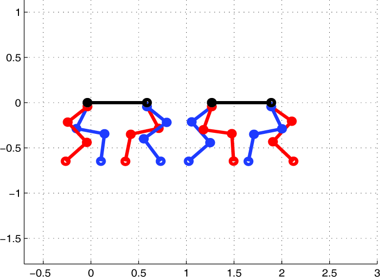
Stick plot of trot gait

Figure 13.

Experiments corresponding to the stick plot

Figure 14.

Hip joint angle of trot gait

Figure 15.

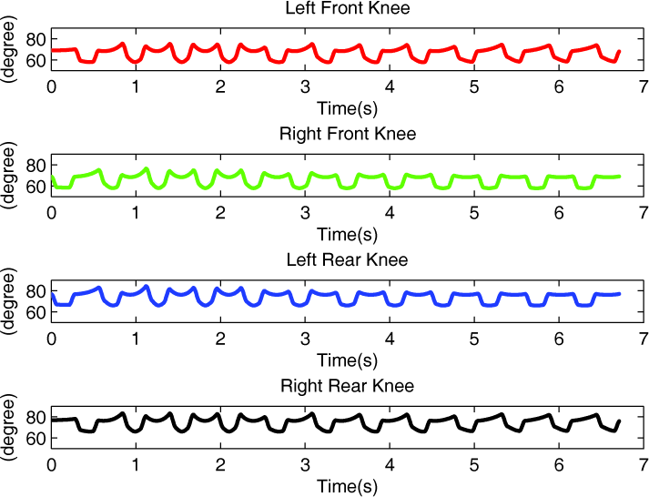
Knee joint angle of trot gait

Figure 16.

Ankle joint angle of trot gait

Though BigDog is capable of trotting at 6.4 km/h with 150 kg payload, quadruped robots controlled by CPG and other methods haven't reached the trotting speed of 3km/h with 50kg payload.

BigDog walks mainly by the movement of knee joint, while hip and ankle move in smaller range. Sometimes we hope that the hip and ankle joint can move in a smaller range, we can rewrite the optimization function: g = (θ₁ - θ₃)². If we need to minimize joint torque, we can design a kind of torque optimization function. Figure 17, 18, 19 show the phase portraits of the states. It is clear that the solution converges to a limit cycle. Simulations and experiments show that the new control method work well with EJ method. New deduction makes EJ method more applicable for different joint lengths.

Figure 17.

Phase portrait of hip joint

Figure 18.

Phase portrait of knee joint

Figure 19.

Phase portrait of ankle joint

5. Conclusions and future work

5.1 Conclusions

In this paper we concentrate on inverse kinematics and a kind of new control method. We also have managed trot gait on the flat ground at the speed of 3km/h with 50kg payload. Three kinds of inverse kinematics method were compared, and EJ method has been proved to lift closed end-effector paths to closed joint angle paths. New deduction of EJ method make it more applicable. The optimization funtion used for the quadruped can minimizes the speed of knee and ankle joint. Simulations and experiments show that EJ method used in Time-Pose control method is realizable in trot gait of quadruped robot.

5.2 Future Work

In our future work we wish to explore how to apply torque for optimization. The highest speed of current method is 3km/h, we hope that the quadruped robot can trot at the speed of 5km/h, with 50kg payload.