
Abstract
Rotor assembly is one of the core components of aero-engine, which basically consists of multistage revolving components. With the influence of parts’ manufacturing errors and practical assembly technology, assembly variations are unavoidable which will cause insecurity and unreliable of the whole engine. Statistical variation solution is a feasible means to analyze assembly precision. When using the three-dimensional variation analysis in rotor assembly, two key issues cannot be well solved, which involve the variation expression (the over-positioning problem of multiple datums) and the variation propagation (revolving characteristic of the rotors). To overcome the deficiency, extended Jacobian matrix and updated torsor equation were derived and unified, which eventually resulted in the improved Jacobian-Torsor model. This model can both provide rotation regulating mechanism by introducing the revolution joint, and characterize the interaction between essential mating features. Multistage rotational optimization of four-stage aero-engine rotors assembly has been performed to demonstrate this solution in statistical way. Results showed that the proposed model was applicable and conducive to precision prediction and analysis in design preliminary stage.
Keywords
Introduction
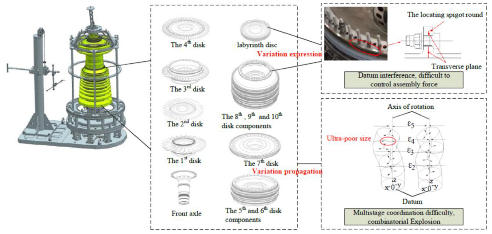
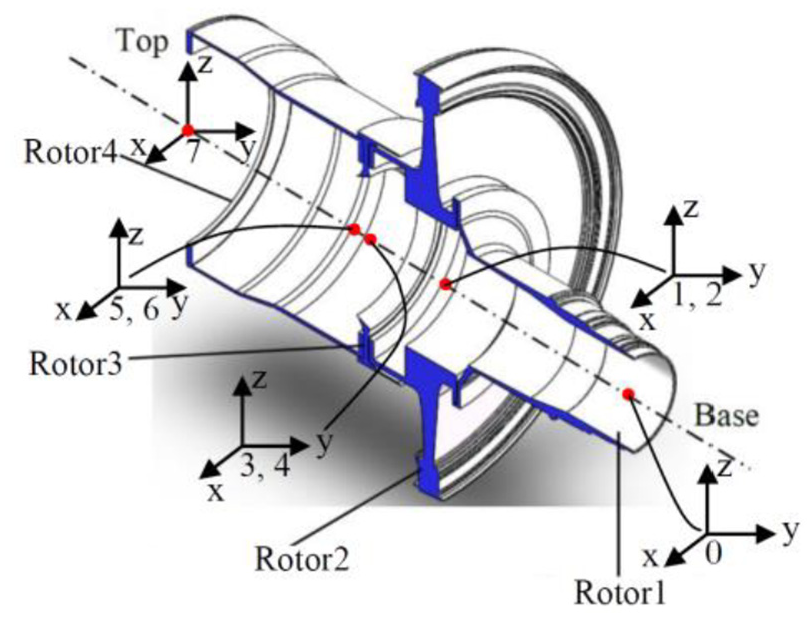
Rotor assembly is one of the core components of aero-engine, which basically consists of multistage revolving components. As shown in Figure 1, the rotor system has universal characteristics of complex internal structure and large number of joins, together with a demand of multiple coordination procedure. Due to the high precision requirement and installation complexity, the rotor assembling workload holds more than thirty percent of the engine’s total workforce.1,2 For instance, the rotor system of GE90-115B aero-engine is made up of 10-stage high-pressure compressor rotors, six-stage low-pressure turbine rotors, and two-stage high-pressure turbine rotors. The tremendous dynamic loads such as vibration load, aerodynamic force, inertia force, torque, etc. will be put on rotors during the service process. If the centering scheme is not designed properly, or parts are unreasonably installed, or the balance test is inefficiency, the engine will appear violent vibration, directly affecting its reliability and security.
Aero-engine rotors assembly.
To maintain the manufacturability and maintainability, aero-engine is produced as a complex assembly of individual revolving components. With the influence of parts’ manufacturing errors and practical assembly technology, assembly variations are unavoidable which will cause insecurity and unreliable of the whole engine. Generally, product quality depends mainly upon the assembly datum, sequence, parts’ type, etc. For aero-engine rotors, they have the rotation properties that every rotor part could be adjusted to a best mounting angle to realize assembly’s optimum concentricity performance. Statistical variation solution is a feasible means to analyze assembly precision. Both in product design stage and actual assembly stage, reasonably building a variation model and proposing a feasible assembly strategy is the effective way to cut down the costs and improve the products quality.
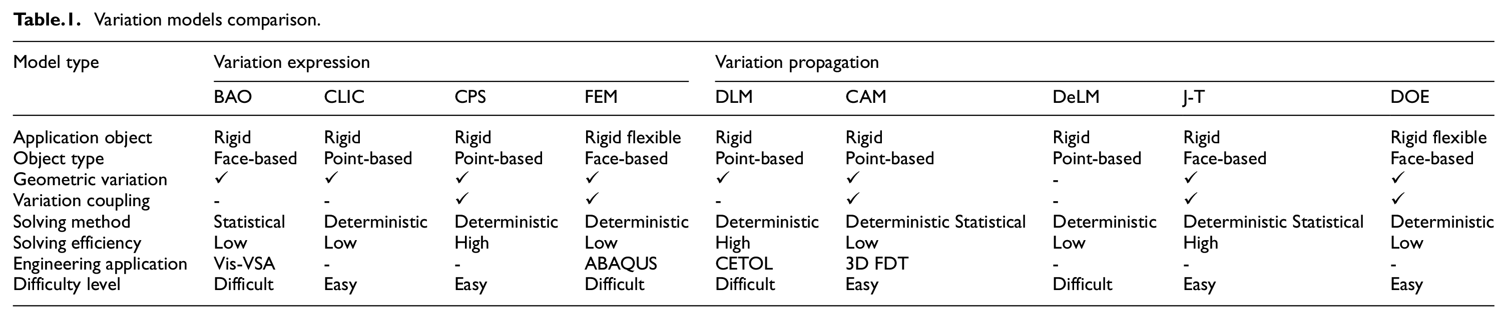
For rotor components assembly, conventional approach of variation analysis focuses on extremum solution and plane dimension chain modeling, which is unable to think about any of the geometrical deviations and the relationship among them; moreover, it overemphasizes the improvement of components’ manufacturing precision, ignoring the optimization method of assembling process. This makes predicted results is too conservative to control fabricating cost and processing difficulty. In fact, due to the inherent complexity of variation propagation, variation accumulation of rotors assembly could be almost not modeled and predicted. A mass of geometric deviations such as orientation, form and location information may be lost. To address this problem, in the past three decades, 3D variation analysis method3,4 develops fast. At the initial stage, kinematic formulation 5 and the network model of zones and datums 6 were first suggested, then there is spatial dimensional chain model, 7 which mainly focuses on the expression of various variations. What followed is variational method8,9 and the direct linearization method 10 ; thereafter the model of Jacobian transfer matrix, 11 torsor,12,13 Tolerance-Map 14 homogeneous transforming matrixes, 15 and the unified Jacobian-Torsor 16 were proposed successively. They provide the basic theories of variation propagation and accumulation based upon the previous study. Recently, the meta-modeling method, 17 polychromatic sets approach 18 and the model of shortest path graph 19 have reached a remarkable development.
The 3D variation model for rotor components assembling needs to solve two issues, involving the variation expression (over-positioning problem of multiple datums) and the variation propagation (revolving characteristic of the rotors). As shown in Figure 1, in aero-engine rotor assembly, the fixing structure commonly uses the transverse plane and the locating spigot round. This connection type consists of a pair of planar feature and cylindrical feather, which will influence and restrict each other. Meanwhile, rotors possess the rotation property that each revolving component can be adjusted to a suitable orientation to meet the desired concentricity performance, thereby causing combinatorial explosion. Some scholars have studied the variation expression of partial features, mainly including: (1) Boolean algebraic operations (BAO): Chen et al. 20 introduced the boolean rules into the variation model, which is suited to analyze statistical solution, but lots of operations such as “union” and “intersection” bring about low computational efficiency. (2) Localization tolerancing with contact influence (CLIC): Chavanne and Anselmetti 21 simulated a group of contact surfaces with virtual extreme points to work out accumulated tolerance. Benichou and Anselmetti 22 further took thermal expansion effect into consideration to research temperature uncertainty. They presented this novel model to avoid partial features interference, but the problem of over-positioning could be not well solved. (3) Contact points-based solution (CPS): Jin et al. 23 improved the small displacement torsor model by introducing contacting points into the conventional torsors. This approach is adopted to simulate rigid parts macroscopically, and is not proper for statistical solution. (4) Finite element method (FEM): Li et al. 24 used FEM to solve the deformations of a novel flexible tooling for aero-engine rotors. Hong et al.25,26 researched air band gap property by adopting the wave finite element model. Andersson 27 explored the supersonic turbines efficiencies by developing a FE model of supersonic blades. Forslund et al. 28 found the relation between thermal stresses and structural stresses by FEM and discussed the functional robustness. But FEM’s modeling is extremely complicated and only used to analyze variation as an assistant.
With regards to variation propagation, scholars have built the mapping relation between parts’ variations and assembly precision from the 3D dimensional chain perspective, mainly including: (1) Direct linearization method (DLM): DLM is fit for describing the variation accumulative process, and Wittwer et al. 29 derived the linear dimensional chain function by expanding the first order taylor series. Yanlong et al. 30 proposed a hybridization of vector loop and quasi-Monte Carlo method to establish the three-dimensional assembly chain. But this model neglected the geometric errors expression. (2) Connective assembly model (CAM): Hussain et al.31–33 made a lot of researches on rotor assembly precision control. They adopted CAM model to control variations accumulation of cylinders. They presented different assembly strategies of parallel assembly and direct assembly, but numerous constraint equations limited the computational accuracy and efficiency. (3) Deterministic locating model (DeLM): Cai 34 combined the linear variational approach to derive the deterministic locating function. It’s essentially an uncertain problem of variation propagation, which is affected by locating points and feature types. (4) Jacobian-Torsor model (J-T): Cao et al. 35 synthesized the advantages about state space theory and torsor model to evaluate rotors assembly precision, and provided the idea of precision compensation. Ding et al. 36 have established the variation propagation path along rotors’ angle and height by improving the Jacobian matrix. However, form and location errors of partial features cannot be fully considered. (5) Design of Experiment (DOE): Judt et al. 37 investigated manual assembly performance of aircraft wing systems, under varying wing structure orientation. Chen et al. 38 analyzed the variation’s abnormality of rotors assembly by using the Pearson theory and Taguchi experiments. Pierce and Rosen 39 have brought machining mode variables into simulated experiments to improve accuracy. Apparently, the efficiency of experiment cannot meet the design requirements.
Table 1 has compared above variation models in detail. It is observed that J-T model is suitable for precision analysis of complex assembly, which includes plenty of geometric variations and connection joints. Rotor parts are commonly contain such assembling features. In consideration of aero-engine rotor’s configuration and assembly characteristic, the J-T theory will be adopted to construct the variation model of revolving components assembly in this article.
Variation models comparison.
However, this method cannot fully solve the issue of composite variations on multiple over-positioning datums. Because of the datum interference and multiple constraints, vector component of each torsor will not be independent any more. In original J-T model, it is common practice to integrate all limited values of tolerancing torsor into account, which is unreasonable and not suitable for statistical analysis. Another problem to be solved is that how to model the rotary characteristics in revolving axisymmetric components assembly. Jacobian matrix can be applied in serial mechanism as the linear arithmetic representation, and can easily map the velocity or displacement of internal joints to the terminal joint. However, it cannot perfectly provide the rotation regulating mechanism for the purpose of this paper.
The main idea for the article is to propose an available model for statistical variation solution in revolving components assembly. Extended Jacobian matrix and updated torsor equation will be deduced and unified to refine the traditional J-T theory, and multistage rotational optimization will be performed using this method in statistical way. By the solution, parts structure attribute and geometric attribute can be fully considered, and statistical concentricity and percentage contribution can be calculated.
Unified J-T model and its improved algorithm
Description of unified J-T model
The traditional J-T model consists of the Jacobian matrix and torsor model. The Jacobian matrix originates from the expression in robot kinematics, which is:
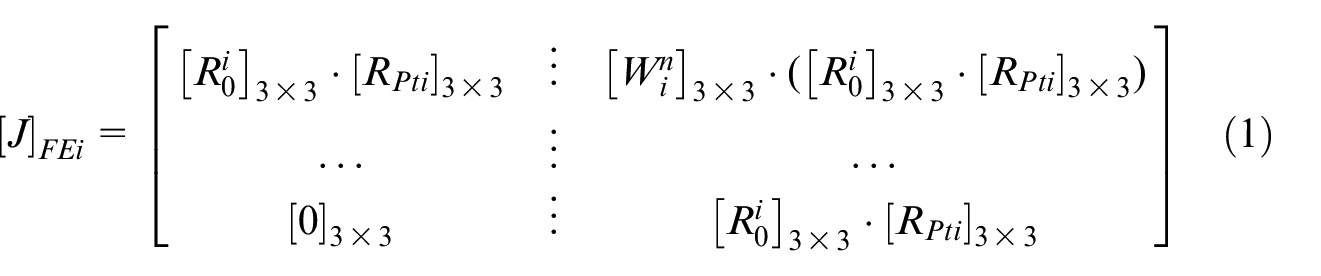
where
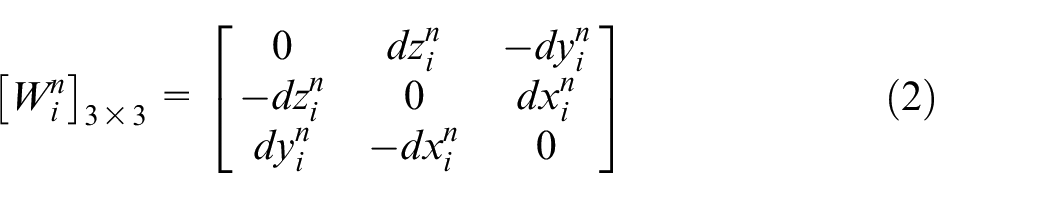
The subscript FEi in [J] means the ith functional element. Two categories of FEs exist in the assembly: internal FE (IFE) and contact FE (CFE). The former denotes two mating features on the same part and the latter denotes two mating features on separated ones. FEs’ Variations could be delivered to the FR (functional requirement) by Jacobian matrix.
Torsor model can describe the ideal position and orientation of any surfaces by three translational vectors and three rotational vectors. Assuming t is the tolerance between arbitrary feature S1 and nominal feature S0, there is:

where u, v, w denote translation vectors along x, y, and z axes; α, β, and γ denote rotation vectors around x, y, and z axes, respectively in local coordinate system.
Hervé 40 presented the displacements set theory, defining the non-invariant degrees, which determined the effective vectors. According to this, some vectors could be taken zero value to simplify the modeling process. Table 2 has shown seven primary torsor forms.
Features and their Torsor models.
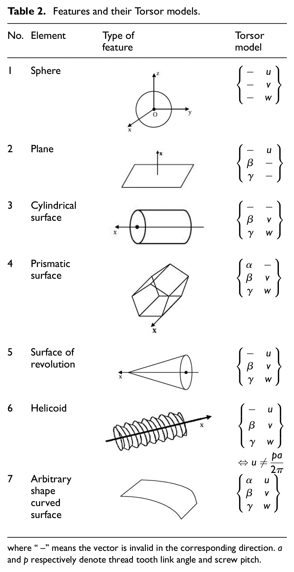
where “–” means the vector is invalid in the corresponding direction. a and p respectively denote thread tooth link angle and screw pitch.
Take No. 3 cylindrical surface as an example. In terms of degree of freedom, it has four effective DOFs in its tolerance zone. According to Salomons’s research, tolerances are only meaningful in directions of all non-invariant degrees. 41 That is, in a torsor model, the number of effective vectors equals to the non-invariant degrees of a feature. More specifically, cylindrical feature originally has six DOFs, but there are only four effective DOFs within its tolerance zone. As shown in Table 2, that is two rotations (α, β) and two translations (v, w). In the tolerance analysis, only these four variations affect the analysis results.
The variation of torsors propagates to the target characteristics taking advantage of Jacobian matrix, which accurately expresses the relative positions and orientations between the local and global coordinates. The unified J-T model takes synthesize advantages of the Jacobian matrix and torsor model. The former is appropriate for variation propagation and the latter is suited to variation expression.42,43 The form of J-T model could be written as:
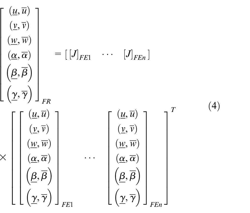
where
Improved algorithm
Extended Jacobian matrix
The classical J-T model described above could not fully apply to the rotating optimization-oriented operation. Concerning this issue, a revolution joint (RJ) is introduced to represent the revolving characteristics of the rotors, by which the extended Jacobian matrix is derived. To be specific, for revolving components assembly, a planar joint combined with another cylindrical joint is most frequently used in the reliable positioning structure, especially in aero-engine rotors assembly. As illustrated in Figure 2, this assembly is composed of two joints which are the planar joint formed by flange plane and shaft end face, and the cylindrical joint formed by locating spigot round. It is actually a revolution joint (RJ) that introduced in this paper. As a result, the RJ simultaneously involves one large planar joint and one short cylindrical joint.
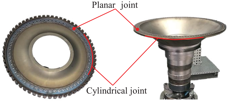
Revolution joint.
In terms of degree of freedom, it is common knowledge that an unconstrained object has six degrees of freedom (DOF), that is, three rotational DOFs and three translational DOFs. Constraints caused by locating or assembling will eliminate some or all component’s DOFs. In the RJ, the planar joint restricts two rotational DOFs and one translational DOF, and the cylindrical joint restricts the remaining two translational DOFs, finally retaining a rotational DOF around rotor’s revolving axis. So in general, the RJ will restrict five DOFs of the rotor part. It should be noted that the DOFs have different meanings in the new RJ and the Cylindrical Feature. The former concerns the mechanism motion constraint in the conventional sense, and the latter concerns the effective vector representation in tolerance semantics and torsor expression.
For n-stage revolving components assembly, the FR results will change while each rotor rotates around its turning spindle axis, and the assembling precision will enhance by selecting an appropriate orientation at each stage. If component i rotates with an angle θi around axes z, the local orientation matrix
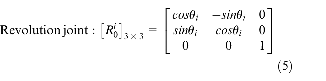
Figure 3(a) and (b) respectively show an n-stage assembly and its connection graph. The global coordinate system 0 and local system i (i = 1, 2, ⋯, n) have been established in the middle of related characteristics. The upper end faces of every part uniformly have a position tolerance TPO (=ti1) and an orientation tolerance TPRA (=ti2). The FR is the accumulated tolerance on the nth rotor’s upper end face along the eccentric direction, measuring in the global reference frame. There are totally n IFEs and (n−1) CFEs which contain (n−1) RJs.
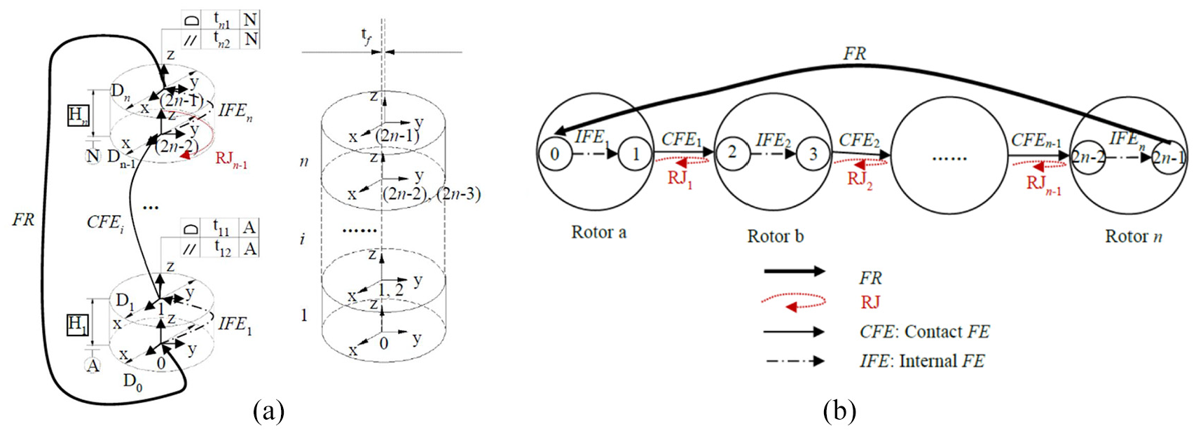
The n-stage assembly: (a) n rotors assembly, and (b) connection graph.
Substituting equation (5) into equation (1), and incorporating the tolerances and dimensions shown in Figure 3(a), the extended Jacobian matrix can be expressed as equations (6) and (7):
where θi denotes the mounting angle of the (i+1)th part with respect to the global coordinates, and Hi denotes the height of the ith part.
The extended Jacobian matrix indicates the vector relation between the torsors of all the FEs and the FR, combining with the multistage mounting angles θi. By virtue of θi in RJ, multistage rotating optimization can be performed and the overall quality of assembly concentricity can be guaranteed.
Torsor equation
Revolving body adopted in this article mainly contains two categories of essential features, respectively are planar feature and cylindrical feature. They cooperate to affect the overall concentricity of assembly.
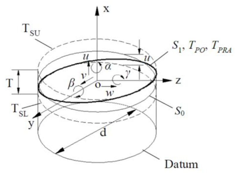
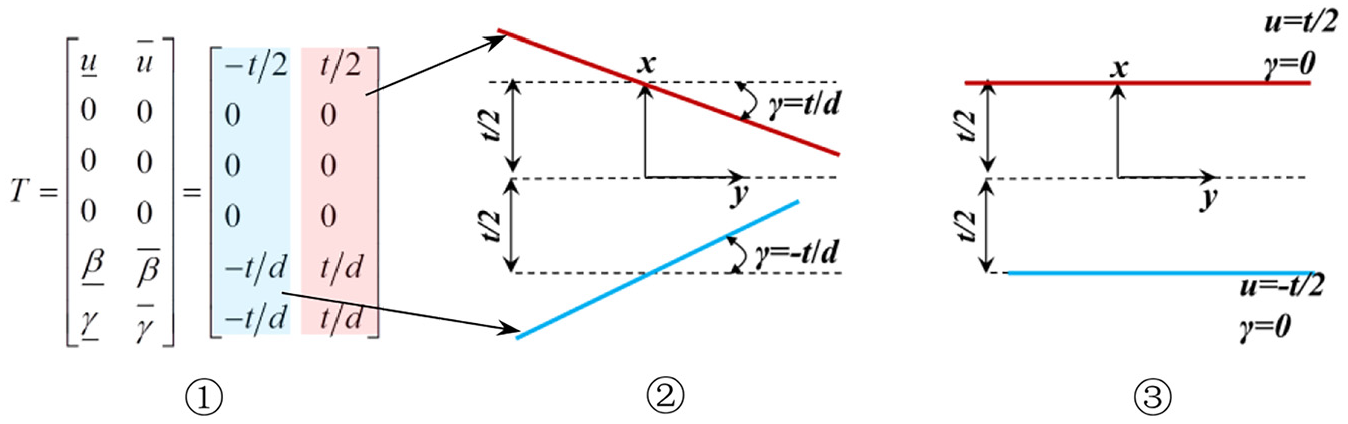
Planar feature between the adjacent matching surfaces constitutes the planar joints, which are selected as a major contact pair. The primary concern in assembling is their contact reliability. Figure 4 shows an individual cylinder. The planar feature contains three invariant degrees, indicating that in its torsor model, three effective vectors still exist in total.
Torsor model of planar feature.
Roy et al. 44 have given the preliminary mathematical derivation of the constraints and variations of planar feature under the independent tolerance constraints. Any variant plane equation can be written as:

First considering position tolerance TPO, the constraint equation of planar feature under position tolerance can be expressed as equation (9):
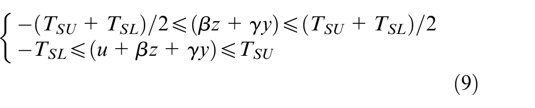
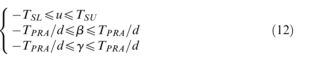
And the variations of the three vectors (u, β, γ) are:
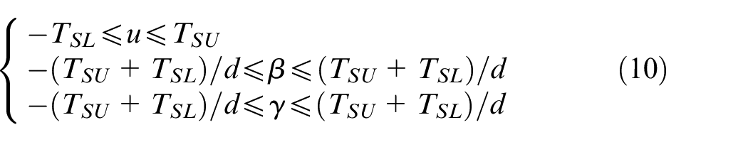
where TSL and TSU denote the limit values of positional tolerances respectively, and their sum is equal to TPO; △x(y, z) = x(yi, zi)−x(yj, zj), and (yi, zi), (yj, zj) ϵ{(−d/2, −d/2), (−d/2, d/2), (d/2, −d/2), (d/2, d/2)}; d denotes cylinder diameter.
Besides TPO, TPRA would also strictly control the feature variation. Composite tolerances must obey the envelop principle (Rule #1, ASME-2009). More specifically, a feature’s rotational displacements resulting from orientation tolerance are essentially subject to the position tolerance. Therefore, the value of orientation tolerance should be smaller than that of position tolerance according to the tolerance standard. In particular, rotational displacements have to shrink to zero when translational displacements reach the maximum value. Figure 5 has shown the detailed process.
The relationship between TPO and TPRA for the planar feature.
Further taking into account TPRA, the torsor’s constraint equations for any rotor’s upper end face could be finally rewritten as equation (11):
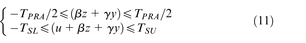
And now, the variations of the three vectors (u, β, γ) are:
As can be seen from equations (11) and (12), the position tolerance mainly limits the translational displacements while the rotations are limited by orientation tolerances. The six vector components of the torsor significantly depend on each other. Furthermore, expressions of other orientation tolerances such as perpendicularity and angularity can be deduced similar to the parallelism.
Cylindrical feature of the revolving component is also constrained by composite tolerance, to ensure that the concentricities of different sections are maintained in a high precision range during the machining process. Figure 6(a) shows a part of an aero-engine rotor. One of the sections is marked with position tolerance φTPO and orientation tolerance φTPRA. According to the envelop principle mentioned above, orientation tolerance is restricted by position tolerance, that is φTPRA≤φTPO. This means when the cylindrical feature reaches the maximum material size, its orientation tolerance φTPRA must be reduced to zero.
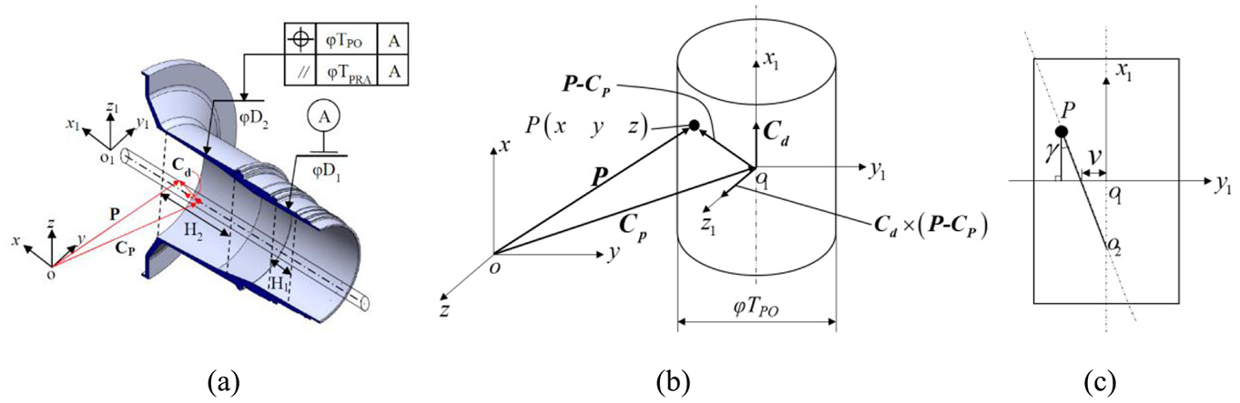
Torsor model of cylindrical feature: (a) rotor part, (b) cylindrical domain of φTPO, (c) plane projection of x1o1y1.
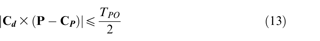
As shown in Figure 6(a), the cylindrical section H2 is restricted by position tolerance φTPO and parallelism tolerance φTPRA, and the cylindrical section H1 is set as datum. According to tolerance semantics, position φTPO mainly restricts the position variation of feature H2’s center line, and parallelism φTPRA further restricts the direction of H2’s center line relative to the datum axis of H1. Therefore, first considering φTPO, the center line with a different position constitutes an envelope cylinder.
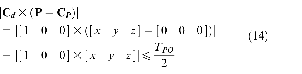
Figure 6(b) shows this magnified cylindrical domain, in which the global reference frame O and local frame O1 are established. Cylindrical region φTPO is the variable range of feature H2’s center line. In the φTPO,
In the local coordinate system O1,
φTPO contains two invariants: translation u along the axis x and rotation α around the axis x, and Figure 6(c) has illustrated the main plane projection of x1o1y1. As shown, the actual axes position of o2P experienced two minor changes: rotate γ around o1z1, and translate v along o1y1. Now the
Combined with small displacement approximation theory, tanβ≈β, tanγ≈γ, the Point
where x∈H2.
And the variations of the effective vectors (v, w, β, γ) are:
where H2 is the length of the cylinder feature.
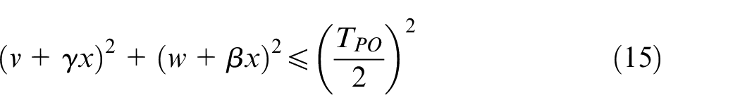
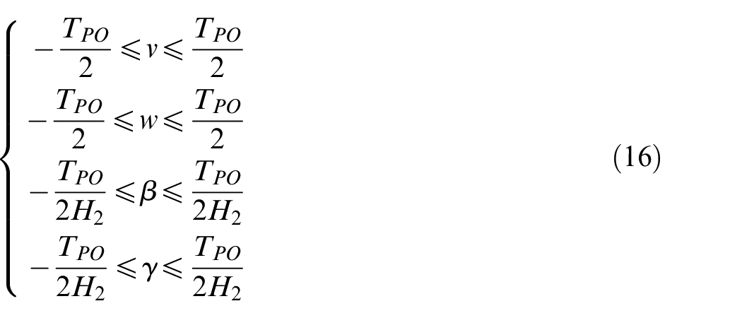
The cylindrical feature is also influenced by the orientation tolerance φTPRA besides the position tolerance φTPO. So the deflection of H2’s center line is further limited by φTPRA, which results in additional constraints on the two rotating vectors β and γ. And the new variation equations are:
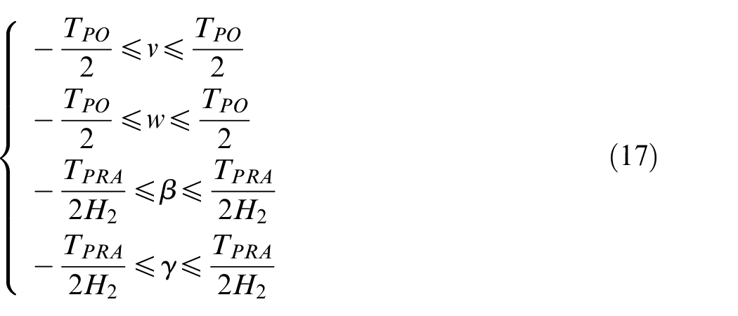
Since the φTPRA does not affect the translation vectors, the variation and constraint equations of v and w will remain unchanged. Equations (15) and (17) are the final torsor equations for the cylindrical feature. The above torsor equations of revolving components ensure that every torsor conforms to the ASME standard and is available to participate in computation statistically. It is beneficial to tolerance specification and allocation of the rotationally symmetric components assembly, such as aero-engine rotors design.
In general, the proposed rule to control the translation degrees and the rotation degrees by a composite tolerance composed of a position tolerance and an orientation tolerance is valid in general, and common in engineering. This is because for precision assemblies, a position tolerance is not sufficient to control both the position and direction of the feature. For example, the feature may deflect the most with the value of TPO when only one position tolerance acts, which result in improper assembly. Therefore, in order to reduce the deflection and meet the special requirements of translation degrees to the greatest extent, an additional orientation tolerance needs to be further applied.
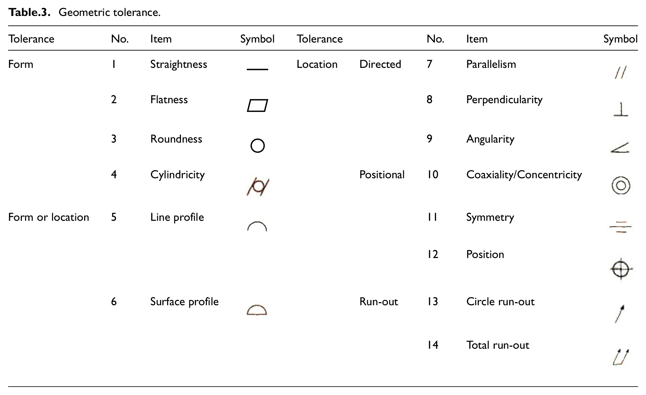
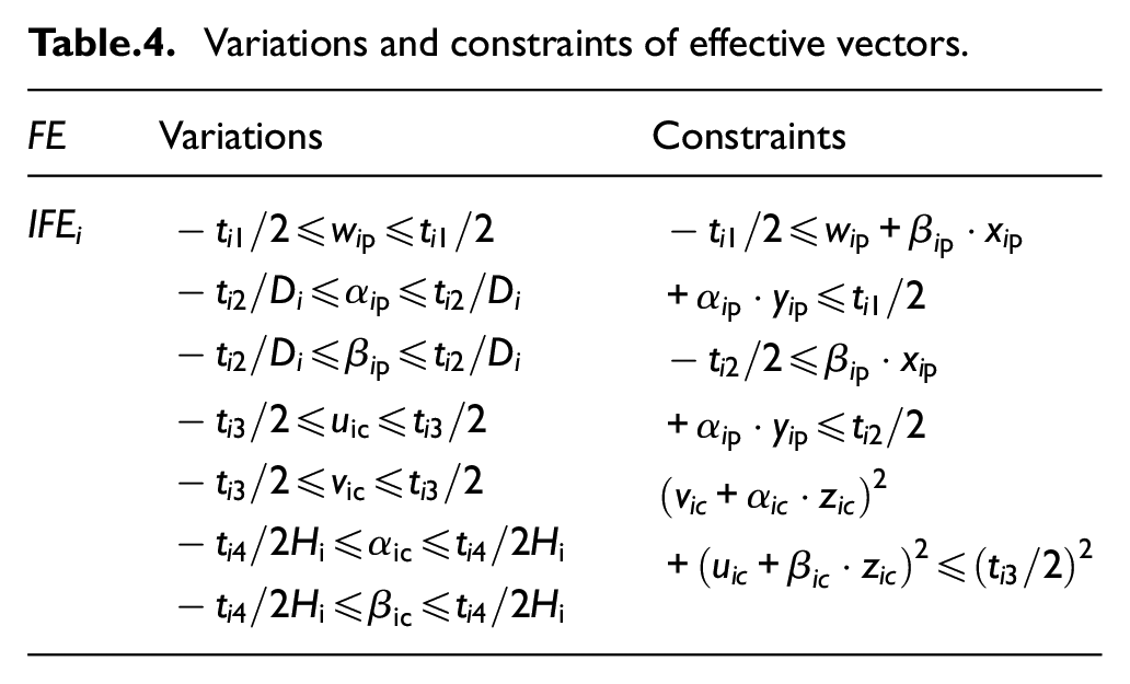
Position tolerance and orientation tolerance include many types, as shown in Table 3. The tolerance combination of position (No. 5, 6, 10, 11, 12) and orientation (No. 7, 8, 9) is a conventional mode. Either way, the mathematical expression is the same, meeting the envelop principle and constraint rule, differentiated only by their tolerance size. To keep generality, we will further summarize the uniform variation equations and constraint equations. Details will be shown in Table 4 for the general revolving components.
Geometric tolerance.
Variations and constraints of effective vectors.
Solution
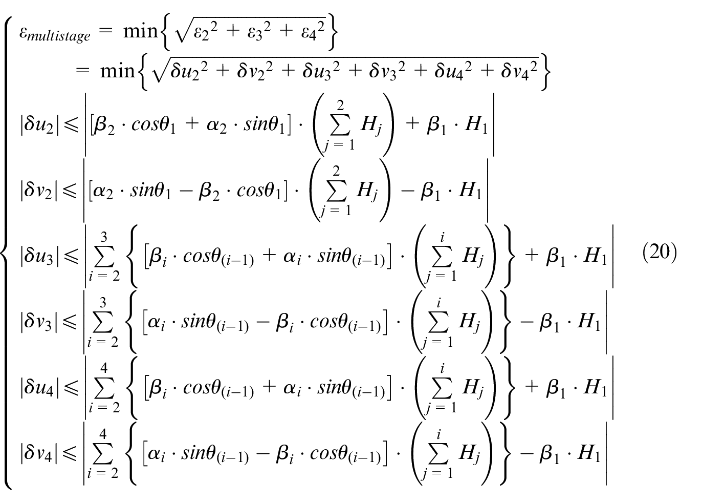
Substituting the extended Jacobian matrixes equations (6) and (7) into equation (4), and combining with the updated torsor equations (11), (12), (15), and (17), the final concentricity variation result of the n-stage rotors assembly is obtained as equation (18):
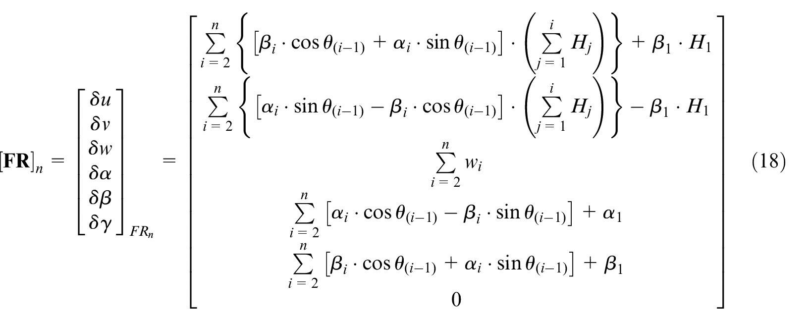
where θi denotes the mounting angle of the (i+1)th part with respect to the global coordinates; Hi denotes the height of the ith part; αi and βi are rotating vectors around x and y axes respectively; wi is the displacement vector on z axes in the local frame.
Taking advantage of δu and δv, which are the vectors along x and y axes, the nth rotor’s concentricity variation could be derived. However, operators pay more attention on the concentricity of the overall assembly rather than that of the top stage rotor only. As illustrated in Figure 7, even if the concentricity of the last stage rotor has been controlled well, other rotors may be also dimensionally out of tolerance.
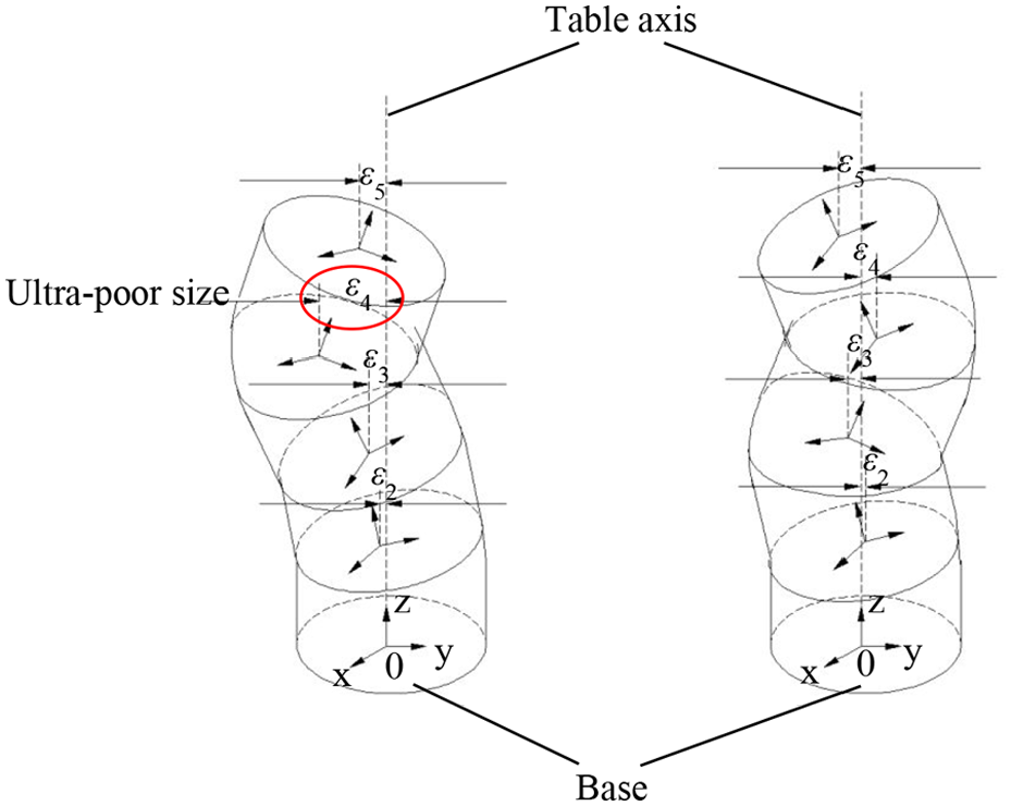
Concentricity control of multistage rotors assembly.
Thus the target eccentricity of the overall assembly can be expressed as equation (19):
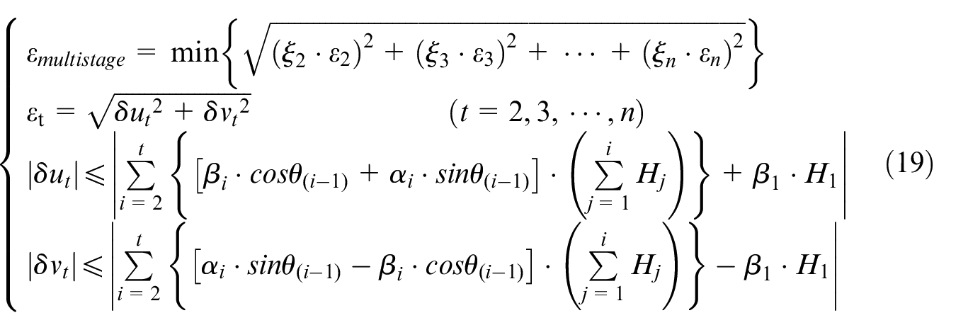
where ξn is the weighting coefficient of concentricity deviation, denoting the nth component’s importance. In this article, all parts are considered equally important, so ξn = 1.
Meanwhile, the variations and constraints of effective vectors for cylindrical torsors should satisfy the requirements of Table 4.
Up to now, the 3D tolerance analysis model for revolving axisymmetric components has been established. Objective function and governing equations for multistage concentricity control have been derived. In order to solve the model, Monte Carlo statistic method is adopted and genetic algorithm 45 is used for seeking optimization. Figure 8 shows the statistical analysis flow chart on the basis of improved J-T model. Details on the analysis procedures of multistage rotors assembly will be elaborated in “Case study.”
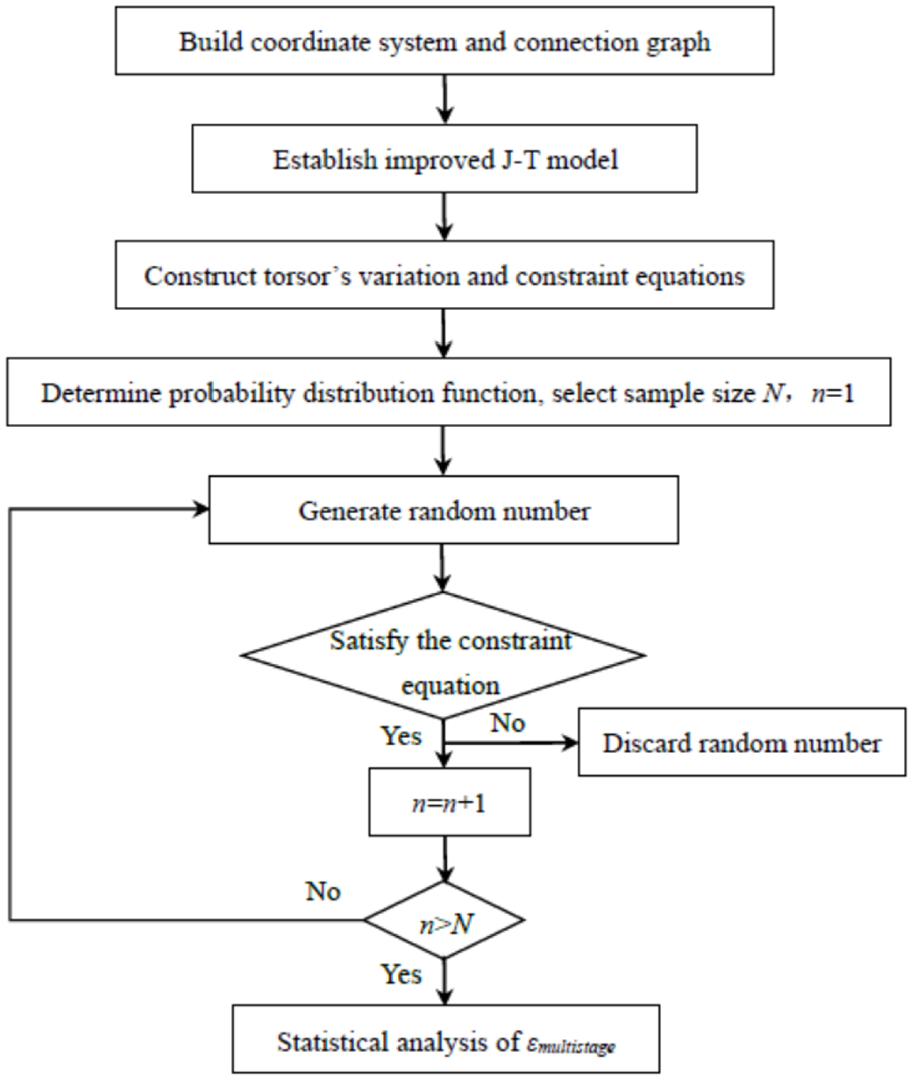
Statistical variation analysis procedure using improved J-T model.
Case study
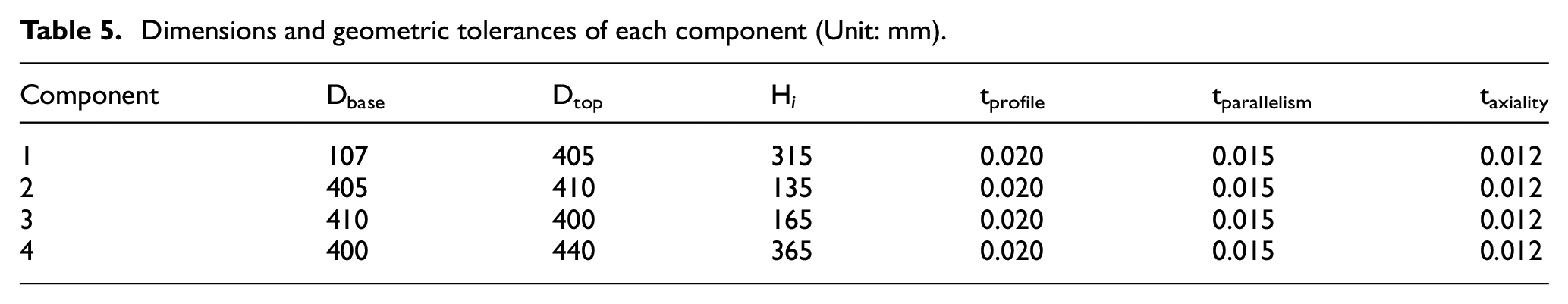
An actual subassembly originating in an aero-engine is used to demonstrate the utility of the improved J-T model. The rotor assembly consists of four revolving components, and all the coordinate systems have been shown in Figure 9. Frame 0 is the global coordinate system and the revolving axis is identified with a line passing through the rotor center. Each component contains a profile tolerance and a parallelism tolerance (located at the upper end of the part, as shown in Figure 3(a)), as well as an axiality tolerance. The specific dimensions and tolerances are listed in Table 5.
Parts drawing of four-stage rotors assembly.
Dimensions and geometric tolerances of each component (Unit: mm).
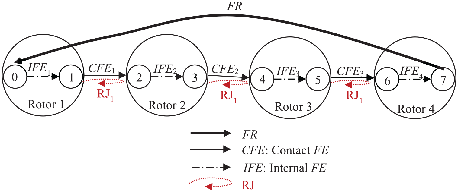
Connection graph of four-stage rotors assembly.
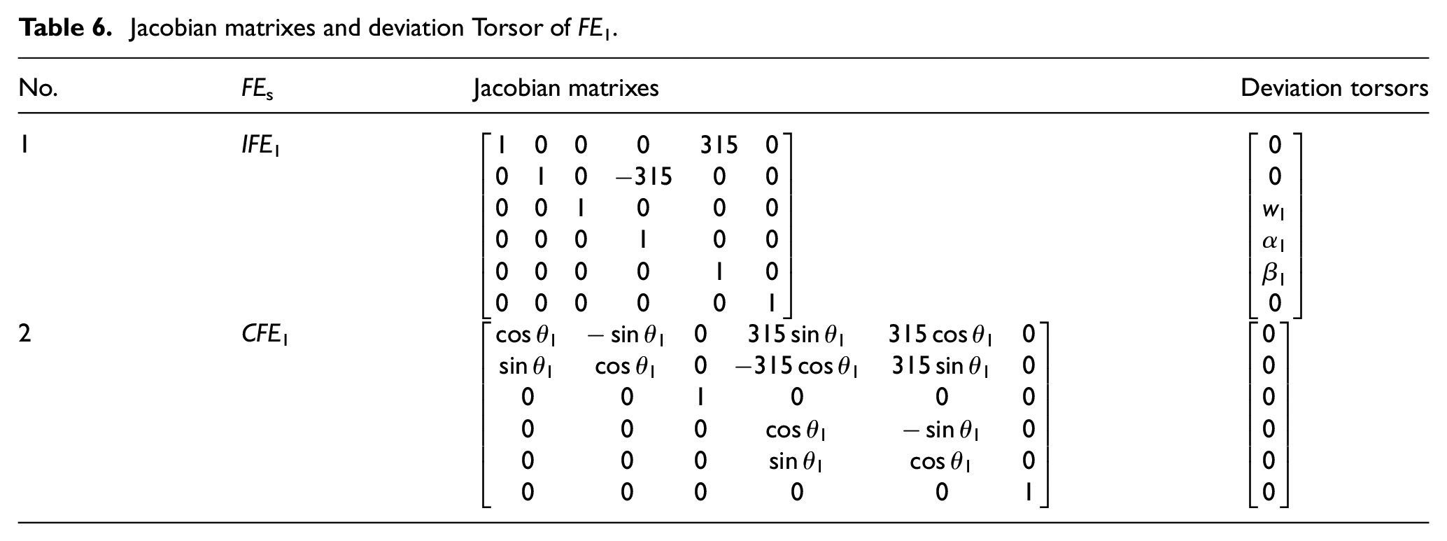
Jacobian matrixes and deviation Torsor of FE1.
Next, the final multistage assembly formula could be derived based on equation (19), as shown in equation (20).
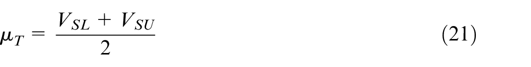
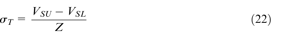
where VSL and VSU are the limit values of deviation torsor. Z denotes the standardized normal value. Here the value of Z is set to 6, indicating that the rejection rate is 0.27%.
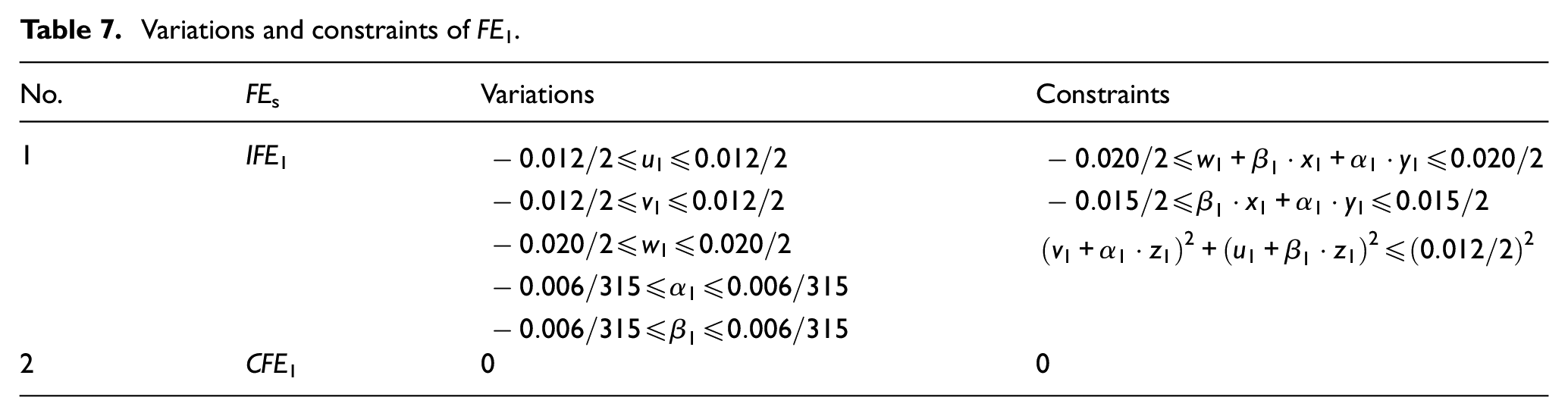
Variations and constraints of FE1.
Statistical results of eccentricity of three variation models (Unit: mm).
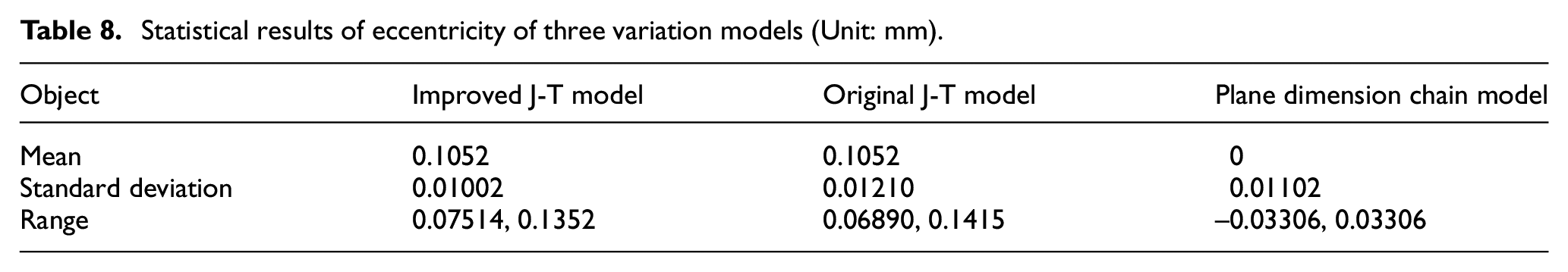
To be specific, the improved J-T model can take interactions of composite tolerances into consideration; original J-T model regards every tolerancing torsor as independent variable, ignoring the mutual effects; plane dimension chain model is a common engineering way based on root sum square (RSS) method, which cannot fully consider geometric tolerances in 2D dimension chain.
Comparison and discussion
Statistical eccentricity analysis
Figure 11 has illustrated the results of Table 8. As can be seen, the variation range of improved J-T model is minimum, that of the plane dimension chain model comes second, and the original J-T model is maximum. This phenomenon is closely related to the standard deviation of the three models. The standard deviation of original J-T model (σ2) is higher than that of improved J-T model (σ1) of 17.2%, while that of plane dimension chain model (σ3) is higher than σ1 of 9.1%. The cause is due to the ineffective management of composite tolerances and lack of study on the common effects between various factors in the original J-T model and plane dimension chain model. Specifically, in the results of σ2 and σ3, it is inaccurate to take limit values of both translational and rotational vectors into calculation. However, σ1 has fully embodied the constraint conditions of composite tolerances, which is much more realistic.
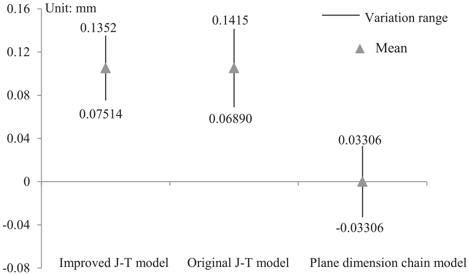
Statistical results of three variation analysis models.
Meanwhile, Table.9 has provided the statistical results εi of each stage rotors. In the table, M-O, T-O, and N-O represent three different assembly strategies of multistage optimization, top-stage optimization and no optimization. The M-O strategy is based on the method proposed in the article, T-O is based on step-by-step strategy focusing on the assembly precision of each top rotor, and N-O is direct-assembly using original J-T model.
Statistical results of eccentricity of three assembly strategies (Unit: mm).
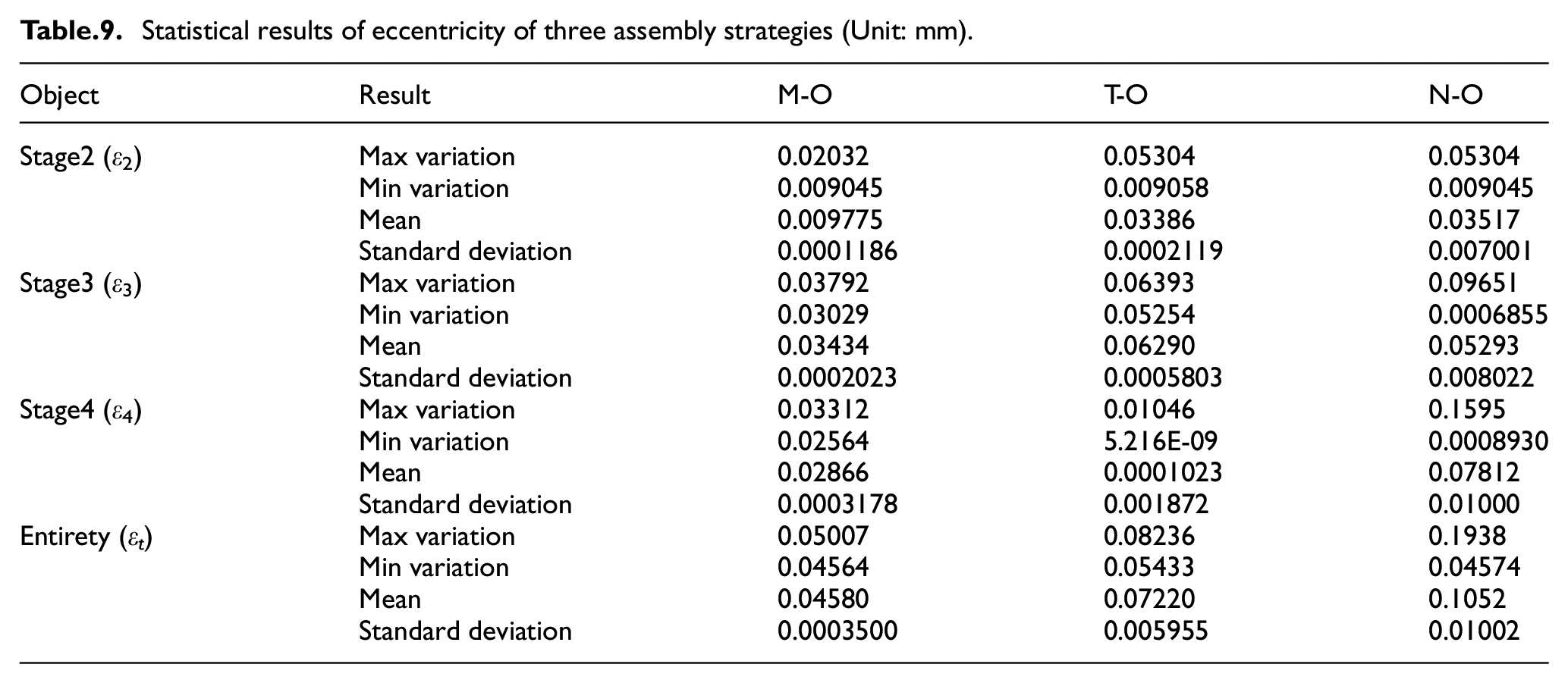
The statistical characteristics of the concentricity deviation shown above are illustrated in Figure 12, involving the mean and standard deviation (see Figure 12(a) and (b)). For the M-O result, its mean value of εt is 0.0458 mm, about 56.5% better than the N-O result; likewise, the concentricity of the second, third, and fourth-stage rotor has been also improved by 72.2%, 35.1%, and 63.3%, respectively from N-O to M-O.
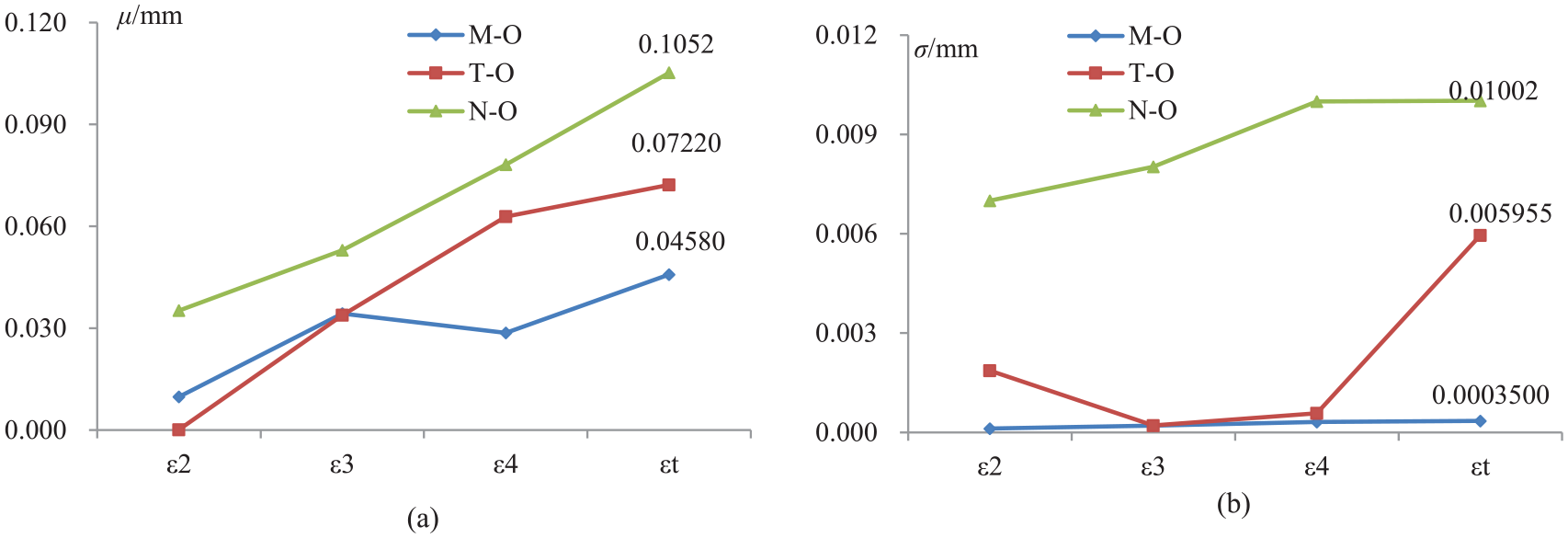
Comprehensive statistical results of eccentricity: (a) mean, and (b) standard deviation.
As described in Figure 7, T-O strategy seems to be not valid to ensure the concentricity of the overall assembly. For the results in four-stage rotors assembly, the average concentricity of the second stage component shows outstanding performance with almost zero eccentricity, seeing Figure 12(a). However, the concentricity worsens at other stages. The concentricity is degraded by 54.4% at stage four and 36.6% at the overall assembly, compared to the M-O result. The above results indicate that the M-O strategy based on the proposed model is efficient and feasible, which could be used in actual assembly process.
As can be seen from Figure 12(b), under the M-O strategy, the minimum value of standard deviation of εt can be achieved, which is 1/17 of T-O result and 1/28 of N-O result. Similar consequences (σ2, σ3, σ4) also happen at the second, third, and fourth stage respectively. This demonstrates that the M-O strategy can make the concentricity level of each part more concentrated, and reduce the systematic risk of assembly failure. It is also observed that the standard deviation has increased as stacking process continues. For instance, the standard deviation of M-O result has increased 41.4% from stage two to stage three, and 36.3% from stage three to stage four. These results suggest that the concentricity controllability and stability become worse, when the rotor gets closer to the top, and the problem of assembly inconsistency is more prominent. Especially, the assembly consistency should be paid more attention in numerous rotors assembly.
The above results illustrate that the multistage assembly strategy based on improved J-T model is conducive to concentricity prediction and control. Meanwhile, this method ensured that the concentricity variation of each rotor has a good consistency and stability, with a higher degree of accuracy.
Probability density distribution analysis
The probability density distribution of assembly variations could be computed on the basis of improved J-T model, and the effect of variation probability type on the ultimate assembling precision can be verified. To validate this, the probability model of FEs are supposed to obey normal or abnormal distributions respectively. Table 10 has shown four combinations of variation distribution model, which will be calculated in the case.
Distribution type and parameters of the FEs.
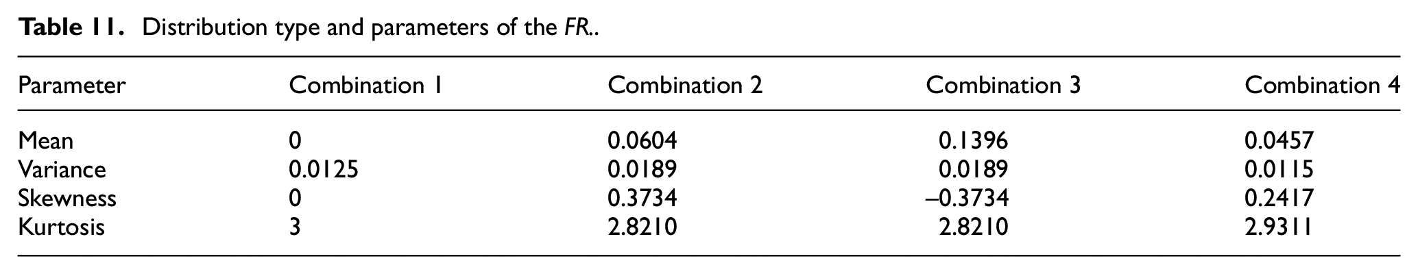
Based on the flow chart in Figure 8, FR’s variation probability type could be solved. Table 11 has shown the results of variation distribution parameters.
Distribution type and parameters of the FR.
With the aid of Monte Carlo (MC) simulation, the variation distribution of the FR can be worked out. The simulation numbers of MC is selected as 10,000 times to maintain efficient and accurate. We assume that the qualified range of FR is (0, 0.038) mm, in accordance with engineering requirements, and the qualification rate of four combinations can be calculated. Figure 13 has illustrated the distribution curve as well as the qualification rate.
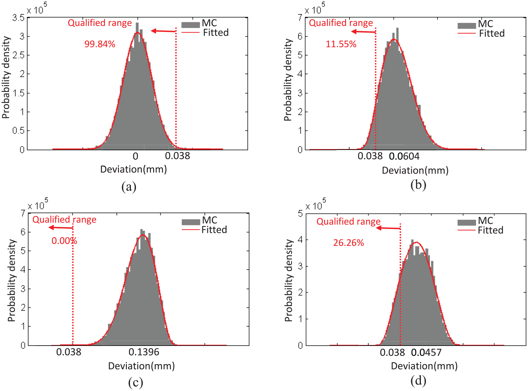
Variation distribution curve and qualification rate: (a) combination 1, (b) combination 2, (c) combination 3, and (d) combination 4.
It is observed that the probability shape of FR’s variation has brought about great changes while the FE’s variation probability type changes. This phenomenon also appears in the aspect of assembly qualified rate. In above four groups of simulations, normal distribution (combination 1) could ensure the qualified rate of up to 99.8%, and the left-skewed distribution (combination 3) almost causes the whole rotors to be unqualified. The reason for the difference is that part’s precision has an overlarge mean shift (=0.1396 mm). All above results have proved that the variation probability type of rotors plays an important role on the ultimate assembly accuracy, and the conventional assumption about normal distribution could not reveal the real variation situation. So the realistically processing capability and assembly technology level is suggested to be considered during the product design phase, to analyze the rotor’s practical variation distribution. Only this can make the results more accurate and credible.
Percentage contribution analysis
Contribution analysis is an important aspect for variation control. It is an effective way for quantificationally observing and controlling the variation propagation. For aero-engine rotors assembly, how to effectively classify parts’ percentage contribution (PC) is the key to improve the overall quality of assembly concentricity. Comprehensively analyzing the contribution effects of each stage rotors can make it clear that which rotor has the most important effect on the precision of the final assembly, so as to avoid repairing or reworking that is caused by the excessive attention to the invalid component’s precision and the incorrect control of the effective component’s precision. For the traditional variation model, the contribution equation could be written as:
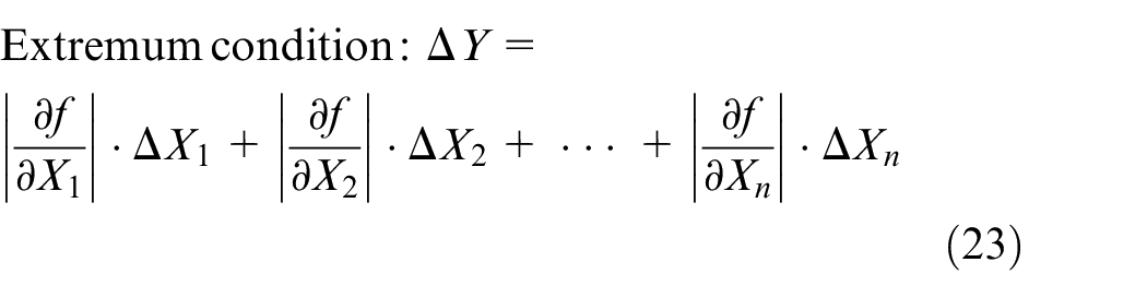
where Y denotes the closed link FR; Xi denotes the ith component link FE; ∂f/∂Xi denotes the sensitivity coefficient of the ith component link FE (i = 1, 2, …, n).
Therefore, the ith FE’s contribution is the ratio of the tolerance value of FE and FR, by multiplying the sensitivity coefficient. The specific expression is as follows:
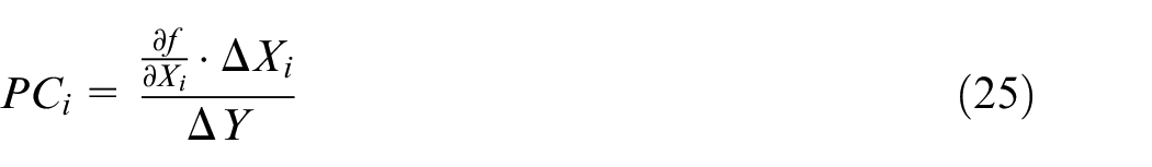
Similarly, the contribution of the component link based on J-T model with extremum condition can be deduced, which is expressed as:
where FR can be considered as the sum of subfunctional requirements FRi (1≤i≤n), which have been derived from equation (4). If each FE’s deviations have been determined, equation (26) can be also regarded as the method to solve the percentage contribution for deterministic deviation problem.
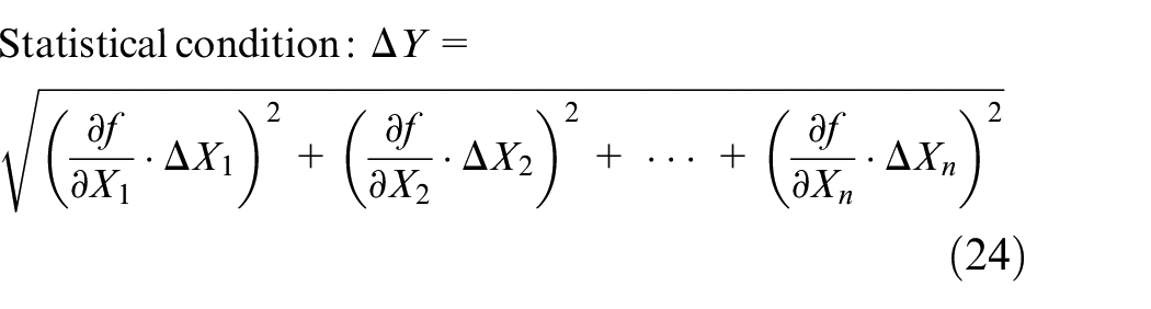
The extremum method is aimed at 100% acceptance rate and parts’ absolute interchangeability. However, in actual assembly, parts’ variations are distributed in different FEs in terms of a certain probability. The statistical method allows a certain reject rate and the existence of incomplete interchangeability. It provides a more relaxed variation environment for the rotor system. This section uses 6σ theorem of the quality management system, which considers that 99.73% variations are in ±3σ range, and its rejection rate is 0.27%.
Similar to the statistical conditional equation (23), the component’s contribution based on improved J-T model in the statistical way is expressed as:
where σFR and σFRi denote the standard deviations of FR and FRi; and the σFR equals to the root sum square of the total FRis’σFRi, that is
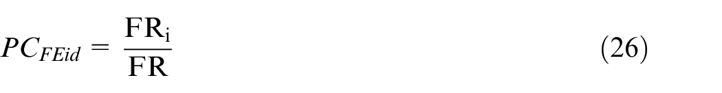
Based on the above analysis, equations (26) and (27) give the contribution calculation method of each component on the basis of J-T model under the extremum condition and statistical condition, respectively. In this case, take the multistage optimization results which have been worked out in Table 9 into equation (27) to calculate the PC FEis . The derived PC and APC (accumulative percentage contribution) have been normalized and shown in Figure 14 in the order of their importance.
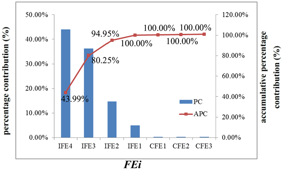
PCs of seven FEs and their APCs.
As can be seen, the IFE4 and IFE3 are the most important factors in the four-stage rotors assembly. The APC of these two FEs is up to 80.25%. This indicates that strictly restricting the first two FEs’ tolerance and appropriately relaxing the nonsignificant FEs’ tolerance would be an applicable way to realize the balance between the quality and the cost for rotors designing. The result is quite helpful for tolerance synthesis and allocation. In addition, it is observed that the PCs of CFEs are all zero, just because in this case the RJ is not given any geometric tolerances.
Conclusion
This article attempts to present a valid variation analysis method for revolving components assembly with multi joints. Extended Jacobian matrix and updated torsor equation were unified. A calculating scheme was illustrated on a realistic case originating in aero-engine subassembly. Following conclusions could be drawn:
The improved J-T model can solve both of variation propagation problem and variation expression issue in revolving components assembly. The extended Jacobian matrix describes the revolving characteristic of the rotor by introducing the revolution joint, and the updated torsor equation characterizes essential mating features of the rotor, involving planar feature and cylindrical feature.
The improved J-T model is convenient for multistage concentricity prediction and control under statistical conditions. By adopting multistage rotational optimization, the overall concentric performance has improved 36.6% relative to the top-stage optimization, and 56.5% relative to directly assembling. Statistical results highlighted the benefits that this approach has a good consistency with the stage numbers, and a better practicality.
This improved model fits probability density analysis and contribution analysis statistically. The result of FR significantly depends on each FE’s variation distribution. In the four-stage rotors assembly, restricting the upper two FEs’ tolerances (APC = 80.25%) and relaxing the rest of FEs’ tolerances is a feasible way to reach a balance between the cost and quality.
Moreover, shortcoming of the proposed method is that, for the rotor structure with the locating spigot round and bolted connection, deformation of working parts under load would be difficult to deal with. In future, the actual contact deformation under certain pre-tension from flange joint bolt and the available number of practical orientations should be taken into account, to model and optimize the actual assembly process, and an effective probabilistic method is needed to improve simulation efficiency, which can be advantageous to guide assembling fulfillment.
Footnotes
Acknowledgements
The authors are grateful for these financial supports.
Declaration of conflicting interests
The author(s) declared no potential conflicts of interest with respect to the research, authorship, and/or publication of this article.
Funding
The author(s) disclosed receipt of the following financial support for the research, authorship, and/or publication of this article: This work was financially supported by the grants from the Fundamental Research Funds for the Central Universities under Grant Number 19D110322, the Open Project of Henan Key Laboratory of Intelligent Manufacturing of Mechanical Equipment, Zhengzhou University of Light Industry under Grant Number IM201905, and the Initial Research Funds for Young Teachers of Donghua University under Grant Number 103-07-0053019.