Sage Journals: Discover world-class research

Abstract

We present the Time-Pose control method for the trotting gait of a quadruped robot on flat ground and up a slope. The method, with brief control structure, real-time operation ability and high adaptability, divides quadruped robot control into gait control and pose control. Virtual leg and intuitive controllers are introduced to simplify the model and generate the trajectory of mass centre and location of supporting legs in gait control, while redundancy optimization is used for solving the inverse kinematics in pose control. The models both on flat ground and up a slope are fully analysed, and different kinds of optimization methods are compared using the manipulability measure in order to select the best option. Simulations are performed, which prove that the Time-Pose control method is realizable for these two kinds of environment.

Keywords

Quadruped Robot Time-Pose control method Trotting Gait Redundancy Optimization

1. Introduction

A quadruped robot has high adaptability and flexibility, not only can it walk on flat ground, but it can also move in unstructured environments. These benefits make the quadruped robot more suitable for a variety of harsh environments, such as disaster relief, military transport and the battlefield. BigDog, developed by Boston Dynamics^[1][2], is the most advanced quadruped robot. Its trotting speed reaches 2.0m/s. A trotting gait is commonly used for low-speed walking, the range of horse trot speed is 1.0–5.0m/s^[3]. Barron-Zambrano's^[4] research on quadruped robots used a walking pattern called the Central Pattern Generator (CPG) for generation of different gaits. However, feedback from the robot has not been considered. In biped robot walking, Cardenas-Maciel^[5][6] designed a T-S Fuzzy Logic Controller and a kind of genetic algorithm for generation of the walking motion. Furthermore Porta García^[7] has proposed an optimal path planning method for an autonomous mobile robot. Robot feedbacks were fully considered in their research. In this paper we present the Time-Pose control method for a trotting gait on flat ground and on a slope. The main idea of the Time-Pose control method comes from the humanoid walk, i.e., we control running speed by step length. Feedbacks of joint angle and velocity are needed in order to form a closed-loop. This method is based on a virtual leg^[8][9], intuitive controller^[10], redundancy optimization and the biped robot Time-Pose control method^[11]. It has two parts: gait control and pose control. Virtual leg and intuitive controllers are introduced to generate the trajectory of mass centre and location of supporting legs in gait control. Redundancy optimization is used for inverse kinematics in pose control.

The Time-Pose control method will be proposed in Section 2 and the definition of the method will be introduced. Gait control will be introduced in Section 3. The models, both on flat ground and up a slope, are analysed so that a unified movement law is generated. Redundancy optimization for pose control is tested by means of a manipulability measure in Section 4. Simulation and experimental results will follow in Section 5. Then the conclusion and the future works will be stated in the last section.

2. Time-Pose control method

The Time-Pose control method drives a quadruped robot by appropriate step length in the right time and right configuration. The Time-Pose control method consists of gait control and pose control. Classification also comes from sensor components, IMU (Inertial Measurement Unit) and sensors on the actuator (i.e., force sensor, position sensor, etc.) corresponding to gait control and pose control, respectively. In gait control, the main objective is controlling the forward speed of the quadruped robot, the outputs are the location of the supporting legs and the trajectory of mass centre for the next gait cycle, while the main objectives of the pose control is solving the inverse kinematics and keeping the torso balanced, the main outputs are joint angle (by the inverse kinematics method) or torque (by the computed torque method), and finally by means of velocity feedback the two control layers are combined together to form a closed-loop control. In this paper we only calculate joint angles in pose control, as indicated by the dotted line in Figure 2.

Figure 1.

Speed for horses. [From Schmidt-Nielsen (1990), redrawn from Hoyt and Taylor (1981)]

Figure 2.

Control diagram of the Time-Pose method

There are many advantages when using the Time-Pose control method. (1) Brief control structure: through gait control and pose control, the task is broken up into small pieces and can be easily understood and managed; (2) high adaptability in different environments: the speed can be controlled in a stable range according to the real terrain, also pose control can guarantee the body's balance; (3) real-time operation ability: the cycle of the gait control is 10ms and 1ms of pose control, the rapidity of the response depends on sample rate of sensors (i.e., IMU, force sensor, position sensor, etc.); (4) anti-interference ability: if an external impact (i.e., heavy impact, kick, etc.) effects the body, the robot will change the touch down location in order to eliminate the impact in the next 10ms period of gait control – 10ms of fast response will greatly ensure the stability of the whole system.

3. Gait control

3.1 Gait control on flat ground

The main movement of the quadruped robot in space is similar to the planar motion. When the robot walks in a specified direction, we only need to control movement in that direction. That equals the planar motion. In this article we mainly concentrate on planar motion control in gait control.

Since it is difficult to study the precise model of a quadruped robot, we find some reasonable constraints which make the complex model equal to a simple model. The simplified model can reduce the degrees of freedom and the complexity of control. How is simplification of the trotting gait model achieved? A trotting gait that causes the four legs to operate in two pairs can be viewed like an equivalent biped gait, because the members of a pair strike the ground in unison and they leave the ground in unison. In order to make the legs work together in pairs, the virtual leg method coordinates the positioning of the physical legs, synchronizes ground contact and equalizes the axial leg force. The geometry of the body also simplifies the task of positioning the physical legs, especially for trotting. The deduction is described in Equation 1. In the process, the mass of leg is ignored when compared to the torso.

\begin{array}{l} f_{x} = f_{1} \sin θ + f_{2} \sin θ - τ_{1} / r * \cos θ - τ_{2} / r * \cos θ \\ f_{y} = f_{1} \cos θ + f_{2} \cos θ + τ_{1} / r * \sin θ + τ_{2} / r * \sin θ - m g \\ τ = f_{1} d \cos θ - f_{2} d \cos θ + τ_{1} + τ_{2} \end{array}

(1)

f, τ, d stand for ground reaction force, hip torque and half of torso length, respectively. If constraint exists:

f_{1} = f_{2}

(2)

Virtual leg can be simplified as follows:

\begin{array}{l} f_{x} = 2 f_{1} \sin θ - (τ_{1} + τ_{2}) / r * \cos θ \\ f_{y} = 2 f_{1} \cos θ + (τ_{1} + τ_{2}) / r * \sin θ - m g \\ τ = τ_{1} + τ_{2}, \\ f = 2 f_{1} \end{array}

(3)

Impose further constraints on virtual leg:

\begin{array}{l} τ_{1} + τ_{2} = 0, \\ z = z_{0} \end{array}

(4)

Equation 3 equals to:

\begin{array}{l} m \overset{..}{x} = f \sin θ \\ m \overset{..}{z} = f \cos θ - m g \end{array}

(5)

The movement law of virtual leg can be simplified:

\overset{..}{x} = g x / z

(6)

The equation above is also the movement law of a linear inverted pendulum. When given an initial condition, the linear inverted pendulum will begin to move by means of gravity. How is the walking speed controlled? The answer is step length – the quadruped's speed will be controlled by selecting different step lengths. The definition of step length is given in Figure 3.

Figure 3.

The simplification of supporting legs

X_{s t e p} = - \dot{X} * T_{s} / 2 - K_{v} (\dot{X} - {\dot{X}}_{d})

(7)

3.2 Gait control up a slope

Gradient is the only difference between flat ground and a slope. How to simplify the model? Because the virtual leg method has no constraints up a slope, so we can apply the same simplification. In this section we set the trajectory of mass centre parallel to the slope and it is an adaptation to the specific environment. The constraint of mass centre is given:

z = k x + z_{o}

(8)

k is the gradient. Substituting Equation 8 into Equation 5, the movement law of the x-axis is:

\overset{..}{x} = g x / z

(9)

There are no differences between Equation 6 and Equation 9; this means that the movement law of x-axis, both on the flat ground and up a slope is consistent. A unified law of x-axis is generated using the virtual leg method. The difference is the speed of z-axis:

\overset{\cdot}{z} = k \overset{\cdot}{x}

(10)

4. Pose control

Achievable configuration is the goal of pose control. Pose control utilizes the output of gait control to solve the inverse kinematics and generate joint motion; this process transfers the desire trajectory of mass centre to the joint angle of legs; and the actual trajectory of mass centre is obtained by substituting the joint variables into the kinematics function (or IMU); finally the actual trajectory is transmitted to pose control, so a closes-loop control is constituted. In Figure 4, a single leg consists of four joints, one in the lateral, three in the forward, that is, there are redundant degrees of freedom in the forward. The main purpose of redundant design includes: (1) bionics design, (2) optimization for kinematics or dynamics. The Jacobian matrix, generated from redundant degrees of freedom, is not square, but rectangular. This means there is no inverse of the Jacobian matrix, so the gradient projection method^[12] is introduced to solve the inverse of the Jacobian matrix.

Figure 4.

Quadruped robot and configuration of one leg, q_i: absolute angle, θ _i : relative angle

4.1 Inverse kinematics of redundant leg

When a leg is redundant, it is certain that the inverse kinematics problem admits infinite solutions. This implies that, for a given location of the leg's end-effector, it is possible to induce self-motion of the structure without changing the location of the end-effector. Thus, the leg can be reconfigured to find better postures for task requirements. Generally speaking, if a motion task trace is commanded to the end-effector, it is possible to continuously modify the joint motion in such a manner that not only the end-effector task is correctly executed, but also a suitable constraint task is managed.

The kinematics mappings for robot legs can be written as:

v = J \overset{\cdot}{q}

(11)

q is the vector of joint variables, v is the vector of task variables.

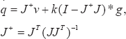
\begin{array}{l} \dot{q} = J^{+} v + k (I - J^{+} J) * g, \\ J^{+} = J^{T} {(J J^{T})}^{- 1} \end{array}

(12)

J⁺ is the pseudo inverse of the Jacobian matrix.

The first item in Equation 12 is a minimum norm solution, the second item is a homogeneous linear equation solution. The first is located in the row space of the Jacobian matrix, while the second is located in the null space of the Jacobian matrix. Therefore, the two items are orthogonal. Since g function can be any self-motion speed, optimization is accomplished by setting the proper value of g.

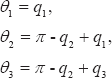
Leg configuration is the key point in calculating the Jacobian matrix. In Figure 5 we set the connection point of the hip and leg as the base coordinate system. Absolute joint angles are selected between the horizontal line and the rod, and relative joint angles are selected between the two rods. Why do we select the hip connection point for the coordinate origin? Because legs not only have a support phase, they also have a swing phase, and it is more convenient for the calculation of these two kinds of movement.

Figure 5.

Sine curve of mass centre

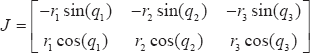
Transformation from work space to joint space:

\begin{array}{l} θ_{1} = q_{1}, \\ θ_{2} = π - q_{2} + q_{1}, \\ θ_{3} = π - q_{2} + q_{3} \end{array}

(13)

The Jacobian matrix can be calculated:

J = [\begin{matrix} - r_{1} \sin (q_{1}) & - r_{2} \sin (q_{2}) & - r_{3} \sin (q_{3}) \\ r_{1} \cos (q_{1}) & r_{2} \cos (q_{2}) & r_{3} \cos (q_{3}) \end{matrix}]

(14)

4.2 Manipulability measure

Redundancy optimization has two evaluation criteria: (1) joint limit in the actual system, (2) a quantitative evaluation function. Redundant legs have more ability than non-redundant ones in many aspects, such as avoiding collisions with obstacles in the working space. In order to make full use of their ability, the manipulability measure^[13][14] is used for evaluation. Measure of manipulability is a scalar value given by:

w = \sqrt{\det J (θ) J^{T} (θ)}

(15)

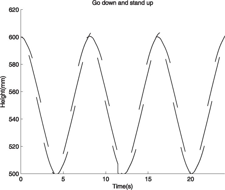
In this section, leg squats are tested by using two different optimization functions. Different functions bring different effects, as we can see in Figure 6. How do we choose a better function? The answer is by using the manipulability measure. The manipulability measure of different functions is given in the next section. The functions are as follows:

g_{1} = [\begin{matrix} - q_{1} + 2 q_{2} - q_{3} \\ 2 q_{1} - 4 q_{2} + 2 q_{3} \\ - q_{1} + 2 q_{2} - q_{3} \end{matrix}], g_{2} = [\begin{matrix} q_{2} q_{3} \\ q_{1} q_{3} \\ q_{1} q_{2} \end{matrix}]

(16)

In the movement the height of mass centre changes as a sine wave and the cycle of sine wave is 8s. The two optimization functions in this test are commonly used, especially g₁ function. There are significant differences in Figure 6. Though the height changes in the same range, the configuration of joints differ from each other. Joint angles in Figure 7 have the same explanation as in Figure 6 and it is more intuitive.

Figure 6.

Plot of squats

Figure 7.

Joint angle of squats

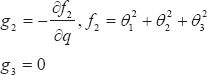
In trotting gait we propose three different optimization functions, the first one is the same as g₁ in Equation 16, and another two functions are as follows:

\begin{array}{l} g_{2} = - \frac{\partial f_{2}}{\partial q}, f_{2} = θ_{1}^{2} + θ_{2}^{2} + θ_{3}^{2} \\ g_{3} = 0 \end{array}

(17)

5. Simulations

For simplicity we ignore the other three legs. The main object, drawn in simulation figures, is a single leg. When walking on flat ground, the gait cycle is fixed to 0.4s and the height of the robot's mass centre remains unchanged throughout. When walking up a slope, the trajectory of the robot's mass centre is parallel to the slope and the angle of the slope is 10 degrees. Since both the movement laws of x-axis are the same, the gait cycle of slope walking can also be 0.4s.

The upper part of Figure 8 shows that after a few steps of acceleration the velocity of mass centre reaches the average of 1.5m / s. The velocity of the following steps is symmetrical. This result also can be inferred from the movement law which is the same as the linear inverted pendulum. In symmetry, we can see that the first half cycle is deceleration and the other half cycle is acceleration. This means that the mass centre decelerates from touching down to middle point, and it accelerates from middle point to lifting off. Why does this happen? Because gravity plays important roles in the process. The bottom half of Figure 8 indicates that the robot stops after three cycles. From Equation 7 we can deduce that step length becomes shorter in acceleration, while it becomes longer in deceleration. Since we need the trajectory of mass centre in gait control, we can get it by integration of velocity.

Figure 8.

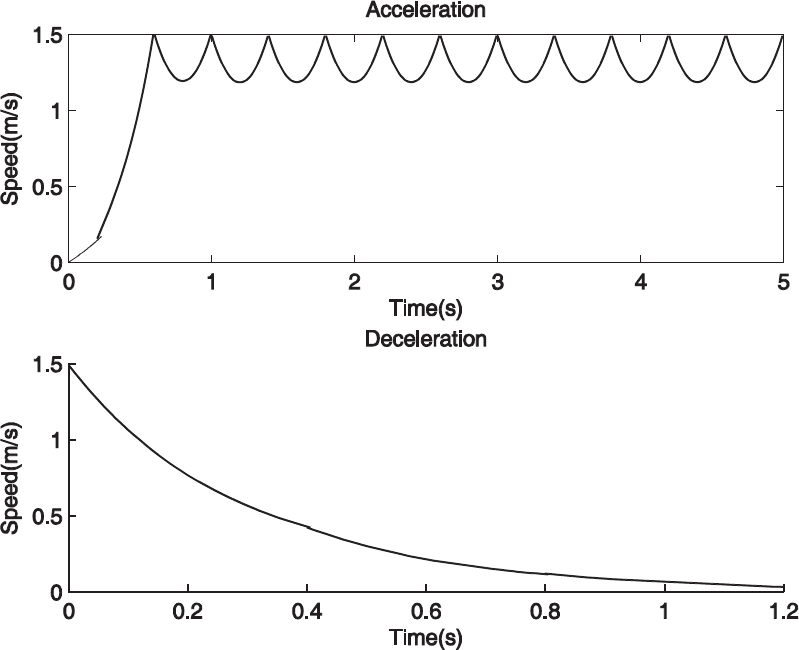
Acceleration and deceleration planning

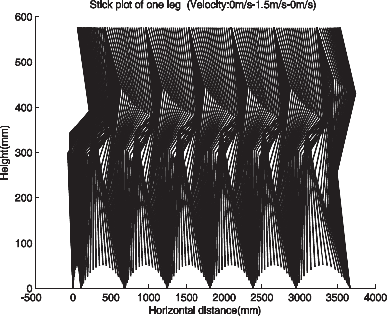
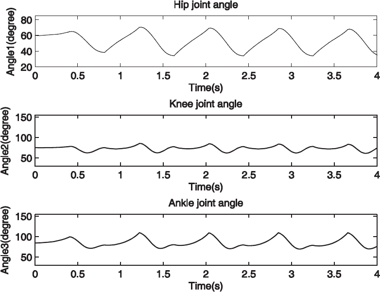
The basic requirement for joint movement is to meet the limit of joint range. The ranges of hip, knee and ankle are 20–85, 40–150 and 40–150 degrees, respectively. From Figure 10 and Figure 13, we know that the movement of the joint is kept at the limit of its range. When walking up a slope, the speed of x-axis is 1.2m/s. In a real system the max speed of hydraulic actuator reaches 300mm/s, while the max speed of the two models is 172mm/s and 162mm/s. So the results can be applied to a real system.

Figure 9.

Plot of acceleration and deceleration

Figure 10.

Joint angle of trotting gait on flat ground

Figure 11.

Manipulability measure of different optimization methods

Figure 12.

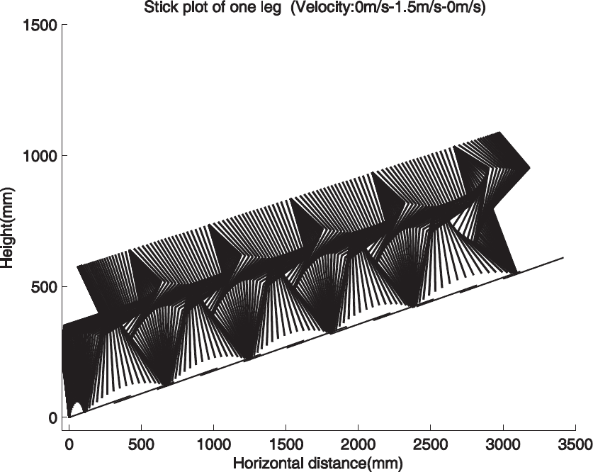
Plot of trotting gait up a slope

Figure 13.

Joint angle of trotting gait up a slope

The manipulability measure in Figure 11 shows that method 1 is the best and method 2 is worse than the benchmark. Because the benchmark function equals zero, method 2 has the opposite effect. So we choose method 1 for walking up a slope. In Figure 12 the leg climbs along the slope and the step length changes consistent with that in Figure 9.

6. Conclusions and Future Work

6.1 Conclusions

In this paper we concentrate on the Time-Pose control method and manage the trotting gait on flat ground and up a slope. These models, by means of simplification, are equal to that of the linear inverted pendulum. The movement law both on flat ground and up a slope has no difference in x-axis. Through use of the manipulability measure we have a better function for redundancy optimization so that in pose control inverse kinematics can be better accomplished. Simulations show that the Time-Pose control method is realizable in the trotting gait of a quadruped robot.

6.2 Future Work

In our future work we wish to explore how to equalize the axial leg force. The current method does not apply torque in pose control; we are currently working on methods for applying torque and redundancy optimization of dynamics.

Footnotes

7. Acknowledgments

This work was supported by the Natural Science Foundation of China (Grant NO._2011AA040801).

References

Boston Dynamics Corp (2008) BigDog, the Rough-Terrain Quadruped Robot. Available: http://www.bostondynamics.com

Boston Dynamics Corp (2008) Bigdog overview. Available: http://www.bostondynamics.com/img/BigDog_Overview.pdf

Collins

J.J.

and Stewart

I.N.

(1993) Coupled nonlinear oscillators and the symmetries of animal gaits, Journal of Nonlinear Science. pp. 349–392.

Barron-Zambrano

J.H.

Torres-Huitzil

(2012) CPG Implementations for Robot Locomotion: Analysis and Design. Robotic Systems-Application, Control and Programming. Available: http://www.intechopen.com/books/robotic-systems-applications-control-and-programming/cpg-implementations-for-quadruped-locomotion-analysis-and-design. Accessed 2012 Feb 03.

Cardenas-Maciel

S.L.

Castillo

Aguilar

L.T.

(2011) Generation of walking periodic motions for a biped robot via genetic algorithms. Appl. Soft Comput. 11(8): 5306–5314.

Cardenas-Maciel

S.L.

Castillo

Aguilar

L.T.

Castro

J.R.

(2010) A T-S Fuzzy Logic Controller for biped robot walking based on adaptive network fuzzy inference system. IJCNN. pp. 1–8

Garcìa

Porta M.A.

Montiel

Castillo

Sepúlveda

(2007) Optimal Path Planning for Autonomous Mobile Robot Navigation Using Ant Colony Optimization and a Fuzzy Cost Function Evaluation. Analysis and Design of Intelligent Systems using Soft Computing Techniques. pp. 790–798

Raibert

M.H.

(1986) Legged Robots That Balance [M]. The MIT Press. Cambridge Massachusetts.

Raibert

M.H.

(1990) Trotting, Pacing and Bounding by A Quadruped Robot. Journal of Biomechanics. 23:79–98.

10.

Pratt

J.E.

Pratt

(1998) Intuitive Control of A Planar Bipedal Walking Robot [A]. Proceedings of the 1998 International Conference on Robotics and Automation [C]. Belgium: [s.n.]. pp. 459–466.

11.

H.X.

(1995) The Research on Dynamic Locomotion of Biped Robot. Thesis. National University of Defense Technology.

12.

Liegeois

(1977) Automatic Supervisory Control of the Configuration and Behavior of Multibody Mechanisms [J]. IEEE Trans. SMC. 7(12): 868–871.

13.

Yoshikawa

(1985) Manipulability of Robotics Mechanism [J]. Inter. J. of Robotics Research. pp. 4 (2): 3–9.

14.

Yoshikawa

(1985) Manipulability and Redundancy Control of Robotic Mechanisms[C]. Proc. of IEEE Int. Conf. on Robotics and Automation. pp. 1004–1009.

Trotting Gait of a Quadruped Robot Based on the Time-Pose Control Method

Abstract

Keywords

1. Introduction

2. Time-Pose control method

3. Gait control

3.1 Gait control on flat ground

3.2 Gait control up a slope

4. Pose control

4.1 Inverse kinematics of redundant leg

4.2 Manipulability measure

5. Simulations

6. Conclusions and Future Work

6.1 Conclusions

6.2 Future Work

Footnotes

7. Acknowledgments

References